Hot-Moments of Soil CO₂ Efflux in a Water-Limited Grassland

Abstract

The metabolic activity of water-limited ecosystems is strongly linked to the timing and magnitude of precipitation pulses that can trigger disproportionately high (i.e., hot-moments) ecosystem CO₂ fluxes. We analyzed over 2-years of continuous measurements of soil CO₂ efflux (Fs) under vegetation (Fs_veg) and at bare soil (Fs_bare) in a water-limited grassland. The continuous wavelet transform was used to: (a) describe the temporal variability of Fs; (b) test the performance of empirical models ranging in complexity; and (c) identify hot-moments of Fs. We used partial wavelet coherence (PWC) analysis to test the temporal correlation between Fs with temperature and soil moisture. The PWC analysis provided evidence that soil moisture overshadows the influence of soil temperature for Fs in this water limited ecosystem. Precipitation pulses triggered hot-moments that increased Fs_veg (up to 9000%) and Fs_bare (up to 17,000%) with respect to pre-pulse rates. Highly parameterized empirical models (using support vector machine (SVM) or an 8-day moving window) are good approaches for representing the daily temporal variability of Fs, but SVM is a promising approach to represent high temporal variability of Fs (i.e., hourly estimates). Our results have implications for the representation of hot-moments of ecosystem CO₂ fluxes in these globally distributed ecosystems.

1. Introduction

Water-limited ecosystems cover over 30% of the land-area of the world and changes in their carbon dynamics could have important impacts on the global carbon budget [1,2]. It is known that the metabolic activity of these ecosystems is strongly tied to the timing and magnitude of precipitation pulse (PP) events at global [3] and regional scales [4,5]. Thus, the study of how water-limited ecosystems respond to different patterns of PPs has been an important research topic for more than 40 years [6], and multiple studies have highlighted the importance of these patterns on ecosystem responses [7,8,9,10]. Despite these efforts, it is still unclear how different types of pulses trigger responses of ecosystem processes [11,12,13], and consequently it is challenging to represent these responses using modeling approaches across water-limited ecosystems [14,15,16].

Climate models project an increase in precipitation variability, including more extreme rainfall events followed by longer dry periods in water-limited ecosystems [17]. These projections have motivated multiple experiments to better understand the role of changes in frequency and intensity of PPs on ecosystem processes [18,19,20,21]. Studies have shown that changes in PPs substantially influence carbon dynamics including net primary production [9], gross primary production [22], net ecosystem exchange [23], ecosystem respiration [24], and soil CO₂ efflux (Fs, as a result of heterotrophic and autotrophic respiration within the soil) [18]. Rapid changes in water availability after a PP could increase the entropy of water-limited ecosystems [25], especially after those initial PPs following a long dry period resulting in hot-moments with disproportionately high Fs [26]. Such PPs could rapidly change soil CO₂ diffusion rates, increase photosynthetic substrate supplies for Fs, and enhance soil microbial and plant metabolism that ultimately increase Fs [8,18,27,28]. The non-stationary nature of these events and the diversity of underlying mechanisms complicate measurement campaigns and modeling efforts [29].

There are several challenges for studying Fs hot-moments triggered by PPs. First, hot-moments are rare events and are constrained by unique biophysical conditions such as antecedent soil moisture [30], PP magnitude [31], and the available substrate supply for microbial respiration [32,33]. Second, hot-moments are sporadic events resulting from a sharp input of a forcing variable (i.e., water input in water-limited ecosystems); therefore, continuous measurements are needed to accurately capture their succinct patterns and magnitudes [15,29,34]. Third, semi-empirical functions based on temperature and moisture responses are commonly used to model Fs [35,36]. These commonly used functions usually fail to represent Fs hot-moments because fluxes could increase >500% in just a few hours versus pre-pulse conditions [29,34]. Considering the attention that water-limited ecosystems have gained for the global carbon cycle [1,2], there is a need for more information on the magnitudes and potential mechanisms of Fs in these globally distributed ecosystems.

The overarching goal of this study is to characterize the influence of PPs that could trigger Fs hot-moments in a water-limited grassland. We analyzed >2-years of continuous measurements of Fs under vegetation (Fs_veg) and at bare soil (Fs_bare). We postulate three interrelated hypotheses: (a) Not all PPs will trigger hot-moments, as hot-moments may depend on the intensity of the PP, pre-pulse soil moisture conditions (e.g., after a long dry period), and canopy metabolism (e.g., during growing season); (b) Soil moisture variability will have higher temporal correlation with Fs than soil temperature in this water-limited ecosystem; and (c) Hot-moments -as non-stationary events- are difficult to represent for semi-empirical models, but machine learning techniques could improve their representation as these methods can account for non-linear relationships. Here, we applied time series analysis to describe the temporal variability of Fs_veg and Fs_bare, and use three modeling approaches ranging in complexity from linear models to machine learning (i.e., support vector machine) to test their potential for representing temporal trends and hot-moments. The ultimate aim of this study is to enhance the discussion of measurement efforts and modeling approaches for Fs hot-moments in these globally distributed ecosystems.

2. Materials and Methods

2.1. Study Site

The Balsa Blanca site is located at 208 m.a.s.l and 6.3 km from the coast, in the Cabo de Gata Natural Park (Almería, Spain; N36°56′26.0′′, W2°01′58.8′′). Following the Köppen classification, the site has a desert climate (Bwh) characterized by the Thermo-Mediterranean bioclimatic zone. The mean air temperature is 18 °C with mean annual precipitation of 200 mm year⁻¹. Bare soil, gravel and rock cover about 49% of the landscape. Vegetation is sparse with 60% cover, and is dominated by the perennial grass Macrochloa tenacissima (L.) Kunth with a mean height of 0.5 m. The rest of the vegetation is composed of Chamaerops humilis, Rhamnus lycoides, and Pistacia lentiscus. The soils are Mollic Leptosols with a sandy loam texture (61.0% sand, 22.8% silt, 19.5% clay), 1.9% organic carbon, 0.16% total nitrogen, 12.2 ratio C:N, 7.9 pH, 1.5% equivalent carbonates, and with a soil bulk density of 1.25 g cm⁻³ in the upper 30 cm of the soil. Analyzed data were collected between June 2011 and November 2013 (i.e., >2 years of measurements) at the study site.

2.2. Instrumentation

2.2.1. Eddy Covariance

Net ecosystem exchange (NEE) was measured using an eddy covariance tower, and we use this information to describe the general metabolic activity (i.e., ecosystem acting as a net carbon source or sink) of the ecosystem during the study period. Previous studies have described in detail the instrumentation, data processing, quality assurance/quality control, and data gapfilling for the study site [37]. Briefly, fluxes of CO₂ were estimated from fast-response instruments (10 Hz measurements) mounted atop a 3 m tower using an open-path infrared gas analyzer (IRGA, LI-7500, Licor; Lincoln, NE, USA). Winds and sonic temperature were measured by a three-axis sonic anemometer (CSAT-3, Campbell Scientific, Logan, UT, USA, hereafter CSI). Data QA/QC and post-processing was performed following standard procedures [38] and described previously for the study site [37]. Storage fluxes were not calculated because the study site has short canopy with well mixing and it is assumed that the storage flux to be zero for a 24 h period. Gaps due to environmental conditions, instrument malfunction and nighttime low turbulence were filled using the marginal distribution sampling technique [39], replacing missing values using a time window of several adjacent days. Positive values of fluxes denote net release to the atmosphere, while negative values indicate net uptake by the ecosystem.

2.2.2. Soil CO₂ Efflux (Fs)

To estimate Fs we measured soil CO₂ concentrations within the soil and applied the gradient method [40]. Because the vegetation cover is sparse we instrumented an area under vegetation (dominated by Macrochloa tenacissima (L.) Kunth) to estimate Fs_veg, and another area with bare soil (situated at 50 cm away from plants) to estimate Fs_bare. We consider that 50 cm away from Macrochloa tenacissima (L.) Kunth is enough to avoid most of the roots as a previous study demonstrated that most roots of Macrochloa tenacissima (L.) Kunth are localized right underneath its canopy [41]. This approach has been followed at the study site by multiple studies to understand spatial variability of FS [42,43]. All solid-state CO₂ sensors (GMM-222, 0–10,000 ppm, Vaisala, Inc., Vantaa, Finland) were installed with a soil temperature probe (107, CSI), and a water content reflectometer (CS616, CSI) at 5 cm depth (i.e., one sensor per depth at each location). All measurements were made every 30 s and stored as 5 min averages.

Soil CO₂ efflux (Fs) was calculated assuming that all transport is due to diffusion [40] as:

$$\mathrm{Fs}=-D_s{\rho }_a\frac{d{\chi }_c}{dz}$$

(1)

where Fs is the upward gas flux (µmol CO₂ m⁻² s⁻¹), D_S the soil CO₂ diffusion coefficient (m² s⁻¹), ρ_a the mean air molar density (µmol m⁻³), $\frac{d{\chi }_c}{dz}$ is the vertical CO₂ molar fraction gradient (ppm m⁻¹). The CO₂ gradient was calculated using the difference between the mean air CO₂ molar fraction (obtained from the eddy covariance tower) and the value of each soil CO₂ sensor. The CO₂ molar fraction was corrected for variations in temperature and pressure. The mean air CO₂ molar fraction was obtained from days when the eddy covariance tower had been recently calibrated and used as a constant for all the studied period, due to the impossibility of using the data continuously due to soiling of the infrared gas analyzer (IRGA) lens. The calibration of this sensor was done monthly using a N₂ standard for zero (purity of 99.999%) and known CO₂ standards for span. We assumed a constant value for atmospheric CO₂ molar fraction, neglecting its small fluctuations that cause negligible errors on the final fluxes [44]. Due to the large difference in CO₂ molar fraction between the soil (when in some cases could be >1000 ppm) and the atmosphere we estimate that the systematic errors could be between 2% and 4% on the final fluxes. The soil CO₂ diffusion coefficient (D_S) was obtained as:

D_S = ξ D_a

(2)

where D_a is the diffusion coefficient of the CO₂ in free air, calculated according to Jones [45], and ξ is the tortuosity. We calculated ξ following Moldrup et al. [46] as:

$$\mathsf{\xi }=\frac{{\left(\varphi -\theta \right)}^{2.5}}{\varphi }$$

(3)

where $\varphi$ is soil porosity and $\theta$ is soil volumetric water content [47]. In this manuscript positive values of Fs denote a CO₂ release to the atmosphere in consistency with NEE measurements.

2.3. Empirical Modeling of Soil CO₂ Efflux (Fs)

We tested three hierarchical approaches to model hourly and daily means of Fs including a simple conditional linear approach, support vector machine (SVM) as a machine learning approach, and an 8-day moving window. First, we modeled Fs_veg and Fs_bare using soil moisture and soil temperature as forcing factors using a conditional approach (referred as Model 1 throughout the text). It is known that water availability is the main controlling factor in water-limited ecosystems, but the temperature dependence of Fs is only relevant when water is not a limiting factor [26,35,48]. Thus, we used the following approach:

If soil temperature > mean annual soil temperature (when the soil is likely to be hot and dry)

log(Fs) = a + b(SM) + c(SM)²

(4)

If soil temperature < mean annual soil temperature (when it is likely to be cool and moist)

log(Fs) = a+ b(Ts) + b(SM) + c(SM)²

(5)

where log(Fs) is either natural logarithm of Fs_veg or Fs_bare, SM is soil moisture in the bare soil or under vegetation, and Ts is soil temperature in the bare soil or under vegetation. This simple approach is likely to represent the temporal trends but unlikely to represent hot-moments of Fs.

Second, we used a support vector machine (SVM) approach using soil temperature and soil moisture as predictor variables for Fs_veg or Fs_bare. This machine learning technique are supervised learning models/algorithms that analyze data for classification and regression analysis. To explore the nonlinear relations of the response of Fs we used a kernel function with SVM. The kernel function was set to be Gaussian and the kernel scale was set to 0.35. We propose that SVM is a flexible approach for exploring nonlinear relations for classification of data and testing its applicability for representing Fs pulses. Previous studies have described in detail the theory behind SVM [49,50] and the application of Gaussian kernels for SVM [51,52]. We cross-validate the classifier using 10-fold cross-validation.

Third, we modeled Fs_veg and Fs_bare using an 8-day moving window (referred as Model 2 throughout the text). Thus, it allows for parameters to shift through time so that projections match the data as close as possible. For this approach, we only applied Equation (5) assuming that temperature and moisture are important within this 8-day moving window. In this case, different parameters for Equation (5) were fitted for each 8-day sliding window calculation. This moving window approach is conceptually analogous to the calculation of ecosystem respiration based on a moving window of nighttime NEE [39]. The selection of an 8-day moving window was based on the fact that the effect of PPs on Fs usually last about 8 days at the study site [27] and this highly parameterized approach could better represent hot-moments of Fs.

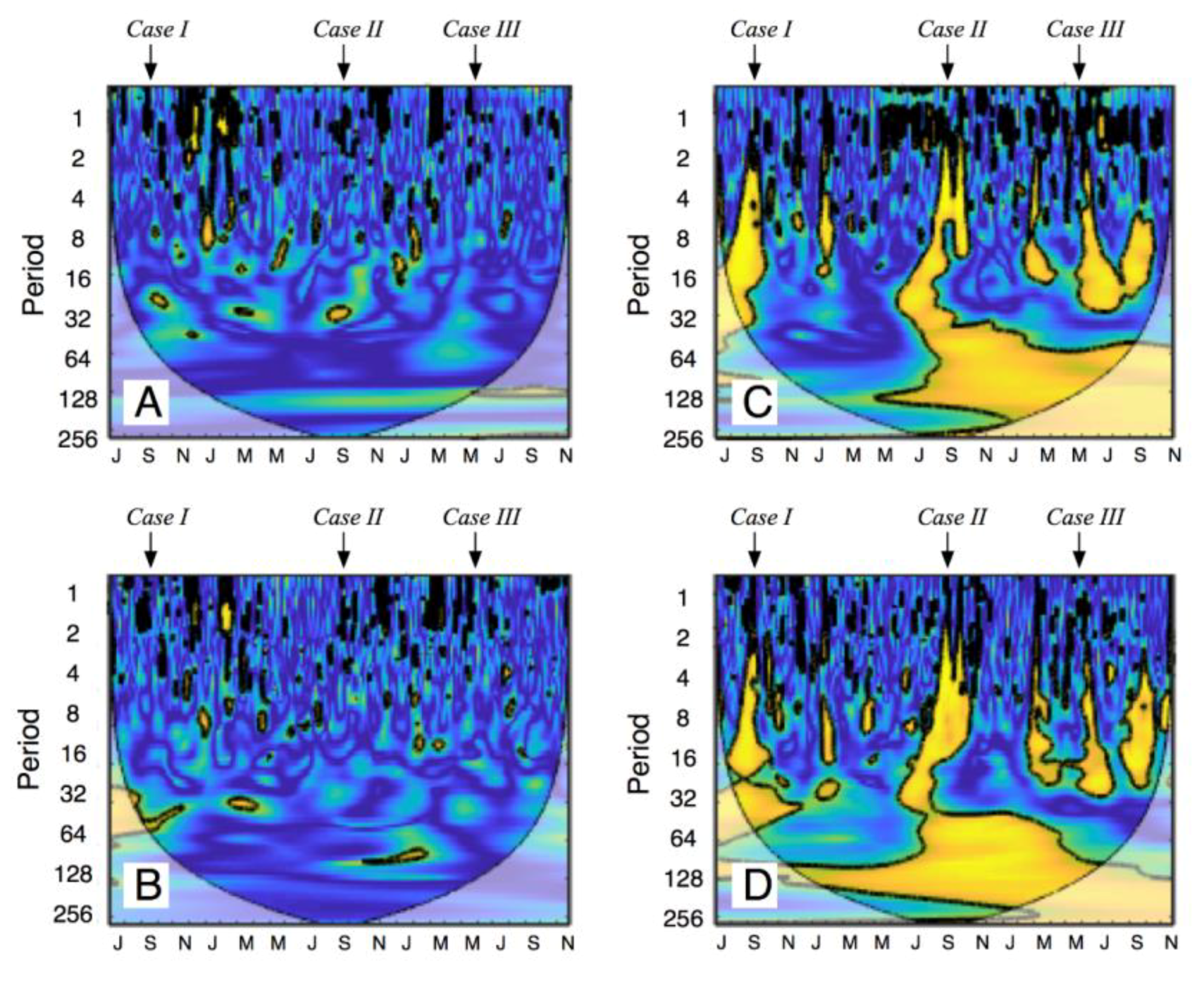
2.4. Time Series Analyses

First, we used wavelet analysis to explore the spectral properties of the times series of Fs (Fs_veg and Fs_bare) and data-model agreement (or disagreement) for Fs_veg and Fs_bare derived from the three empirical approaches described above. Wavelet analysis is a time series technique that has been widely applied in the geosciences [53], and recently utilized to analyze the temporal variability of ecosystem-scale fluxes [54,55,56], soil CO₂ effluxes [15,57], and to identify data-model agreement [57,58,59]. This technique is used to quantify the spectral characteristics of time series that may be nonstationary and heteroscedastic. Specifically, we used the continuous wavelet transform because of its ability to produce a smooth picture in the frequency domain of a time series (e.g., soil CO₂ efflux, data-model residuals) and its suitability for visual interpretation. The ability to discern small intervals of scales (i.e., spectral resolution) depends on the choice of the mother wavelet function. For this, we used the widely used Morlet wavelet, a complex nonorthogonal wavelet with a good time and scale resolution that has been widely used for geophysical applications [53,60], and biometeorological measurements [57,58,59]. We first analyzed time-series of measurements using a 1-h time step and then model residuals using a 1-day time step.

Second, to test the potential influence of soil temperature or soil moisture on Fs, we explored their partial temporal correlation with Fs_veg or Fs_bare. In other words, we explored the temporal correlation of Fs with soil temperature taking into account the influence of soil moisture and vice versa. We applied partial wavelet coherence analysis (PWC), as it can be interpreted as a technique similar to partial correlation that can identify significant temporal correlations between two different time series after eliminating the influence of a third one. Previous reports have described the PWC in detail for climate studies [61]. The statistical significance (5% significance level) of common power between any two time series was assessed for PWC using 1000 Monte Carlo simulations of white noise time series [60]. The time-series used for PWC were analyzed using a 1-h time step.

3. Results

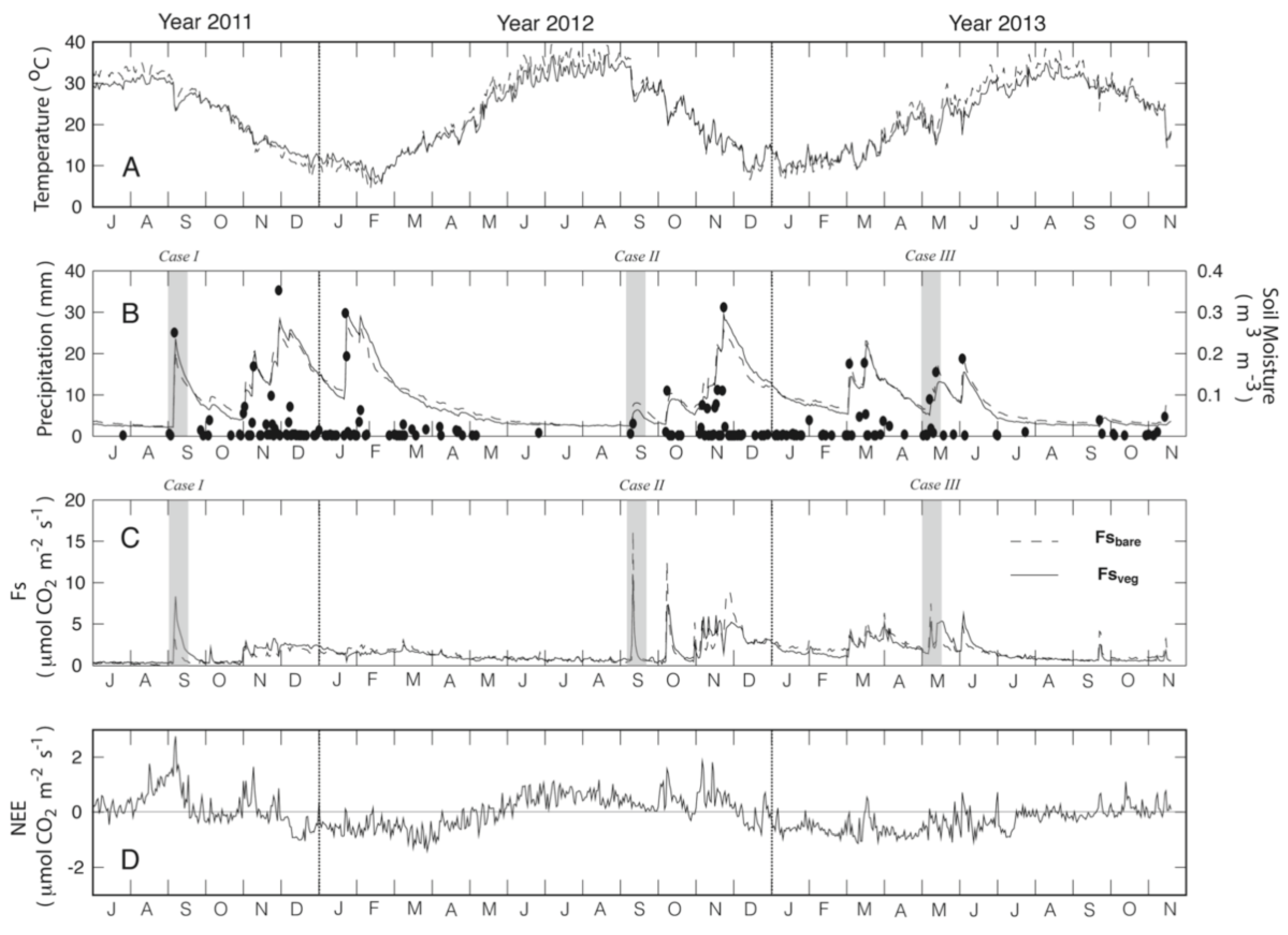
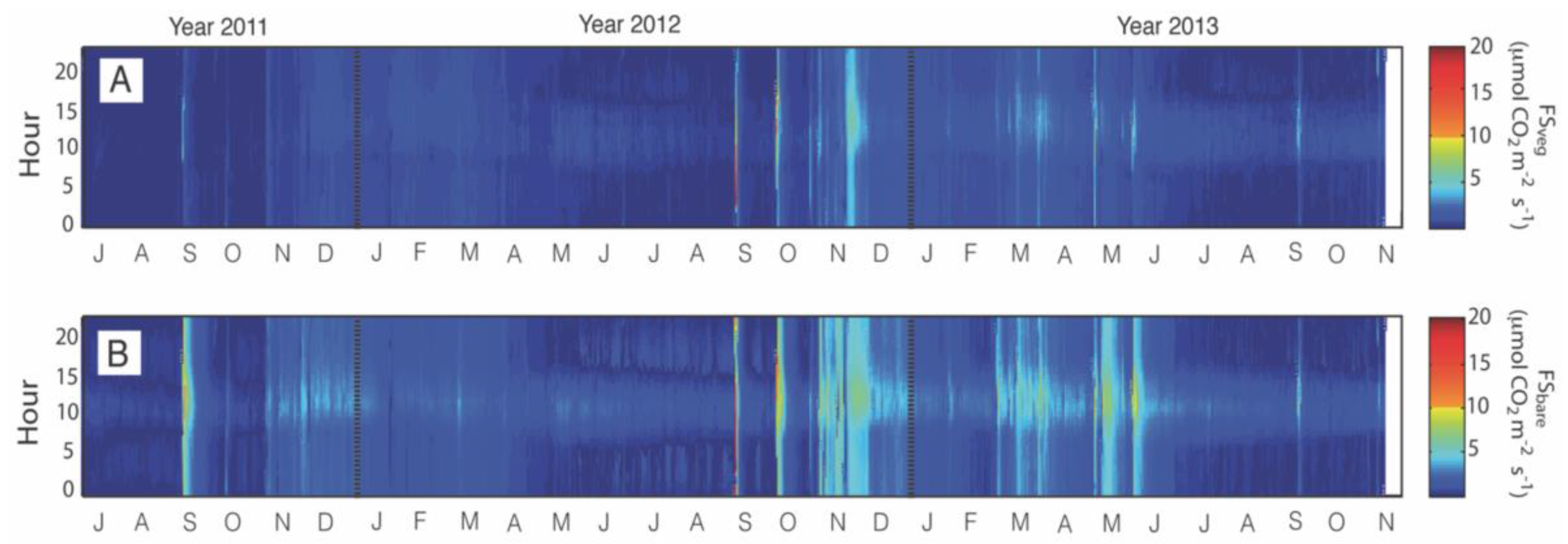
3.1. Description of Temporal Patterns

Daily soil temperature ranged from a minimum of 5 °C and a maximum of 38 °C; with an annual mean of 22 °C under vegetation and 23 °C for bare soil (Figure 1A). Between September 2011 and August 2012 (first hydrologic year) the study site received 216 mm of precipitation, and between September 2012 and August of 2013 (second hydrologic year) it received 221 mm (Figure 1B). There were no substantial differences in total precipitation between the hydrological years, but the distribution of the PPs resulted in different patterns of soil moisture along the years (Figure 1B).

Water pulses following the dry season (between September and October) substantially raised Fs_veg and Fs_bare (Figure 1C). The overall mean for Fs_veg and Fs_bare was 1.5 ± 1.4 µmol CO₂ m⁻² s⁻¹ but hot-moments were present with instantaneous values >20 µmol CO₂ m⁻² s⁻¹ (Figure 2A,B). We analyzed the cumulative sum of Fs based on hydrologic years (see above). Annual Fs_veg was 480 and 819 gC m⁻², while annual Fs_bare was 431 and 871 gC m⁻² for the first and second hydrologic years, respectively. Positive NEE values were common during the dry season when the ecosystem acted as a net CO₂ source to the atmosphere (Figure 1D).

We explored the spectral characteristics of the time series of Fs_veg and Fs_bare (Figure 3). Results using wavelet analysis demonstrate that the 1-day period for Fs_veg is more constant than for Fs_bare (Figure 3A,B). We observed three distinct PPs that substantially influenced the spectral signature of Fs. First, the large precipitation pulses at the beginning of each growing season (i.e., September) resulted in discrete hot-moments influencing the periodicity for Fs_veg (Figure 3A) and Fs_bare (Figure 3B) between a time-period of 1-to 16-days (pulses Case I and II). Arguably, another “hot-moment” is observed during October of 2012, but for the purpose of this study (and to simplify the discussion) we consider it similar to a Case II and therefore is not further analyzed. Second, the large precipitation pulse during the growing season of year 2013 also influence the periodicity for Fs_veg and Fs_bare between 1-to 8-days time-periods (pulse Case III).

3.2. Influence of Soil Temperature and Soil Moisture on Fs

Using PWC analysis we found a lack of consistent temporal coherence between Fs_veg or Fs_bare with soil temperature when considering the effect of soil moisture (Figure 4A,B). In contrast, we found significant temporal coherence between Fs_veg or Fs_bare with soil moisture when considering the effect of soil temperature (Figure 4C,D). The temporal coherence was clearly influenced by PPs for Case I, II, and III with significant temporal correlations between 1-and 16-day periods. The seasonal influence of soil moisture on Fs is represented by the temporal correlation at scales > 128-days (Figure 4C,D).

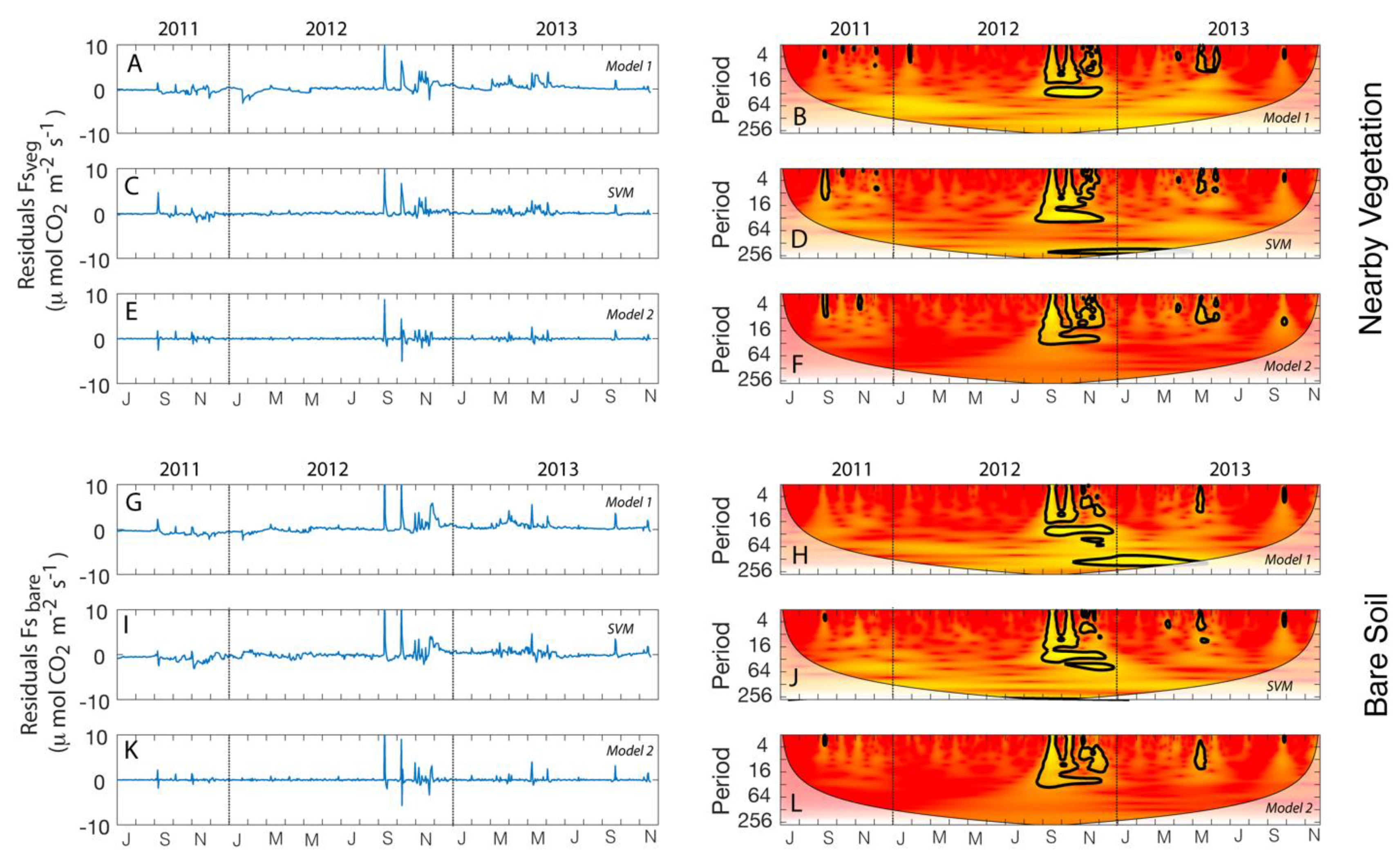
3.3. Modeling Daily Fs

3.3.1. Model 1

Using the conditional approach for Equations (4) and (5) with daily Fs_veg values resulted in an explained variance of 47%, with a RMSE of 0.49 µmol CO₂ m⁻² s⁻¹. The continuous wavelet transform shows that errors in the residuals were focused on hot-moments during PPs with periodicities ranging between 2-and 16-days (Figure 5A,B). These underestimated hot-moments correspond to the PPs previously identified as Case I to III. This model has a larger probability to over represent Fs_veg values of ~1.5 µmol CO₂ m⁻² s⁻¹ and under represent Fs_veg values > 3.0 µmol CO₂ m⁻² s⁻¹ when compared to measurements (Figure 6A). Considering the full 2-years of measurements, the model underestimates the cumulative Fs_veg flux by 12% mainly by over representing Fs_veg values for year 2011 and underestimating Fs_veg values of years 2012 and 2013 (Figure 6B).

Using this approach for Fs_bare resulted in an explained variance of 35% and a RMSE of 0.67 µmol CO₂ m⁻² s⁻¹. The continuous wavelet transform also shows that errors for Fs_bare residuals were focused on hot-moments that correspond to the PPs previously identified as Case I to III (Figure 5G,H). This model also has a larger probability of overestimating Fs_veg values of ~1.5 µmol CO₂ m⁻² s⁻¹ and underestimating Fs_veg values > 2.5 µmol CO₂ m⁻² s⁻¹ when compared to measurements (Figure 6C). Considering the full 2-years of measurements, the model underestimates the cumulative Fs_bare flux by 15% mainly by overestimating Fs_bare values for year 2011 and underestimating Fs_bare values of years 2012 and 2013 (Figure 6D).

3.3.2. Support Vector Machine (SVM)

Using SVM, we were able to explain 71% of the variance of Fs_veg with a RMSE of 0.7, and 51% of the variance of Fs_bare with a RMSE of 0.98 µmol CO₂ m⁻² s⁻¹. The continuous wavelet transform shows that errors in the residuals were also focused on the previously identified Cases I to III for Fsveg (Figure 5C,D) and Fs_bare (Figure 5I,J). This model also has a larger probability of overestimating Fs values of ~1.5 µmol CO2 m⁻² s⁻¹ and underestimating Fs_veg values > 2.5 µmol CO2 m⁻² s⁻¹ when compared to measurements (Figure 6A,C). Considering the full 2-years of measurements, the model underestimates the cumulative Fs_veg flux by 7% and underestimates Fs_bare by 1% as a result of error cancelation. This approach overrepresents Fs values for year 2011 and underestimates Fs values of years 2012 and 2013 (Figure 6B,D).

3.3.3. Model 2

Using the 8-day moving window approach with Equation (5), we were able to explain 84% of the variance of Fs_veg with a RMSE of 0.52, and 48% of the variance of Fs_bare with a RMSE of 0.73 µmol CO₂ m⁻² s⁻¹. The continuous wavelet transform shows that errors in the residuals were also focused on hot-moments during PPs with periodicities ranging between 2-and 16-days (Figure 5E,F). These underestimated hot-moments also correspond to the PPs previously identified as Case I to III.

This model has a similar probability density function for Fs_veg values when compared to measurements (Figure 5A), but slightly overestimates Fs_bare values of ~1.5 µmol CO₂ m⁻² s⁻¹ and underestimates Fs_bare values > 3.0 µmol CO₂ m⁻² s⁻¹ when compared to measurements (Figure 6A,C). Considering the full 2-years of measurements, the model underestimates the cumulative Fs_veg flux by 2% and underestimates Fs_bare by 3% as this approach closely followed the measurements (Figure 6B,D).

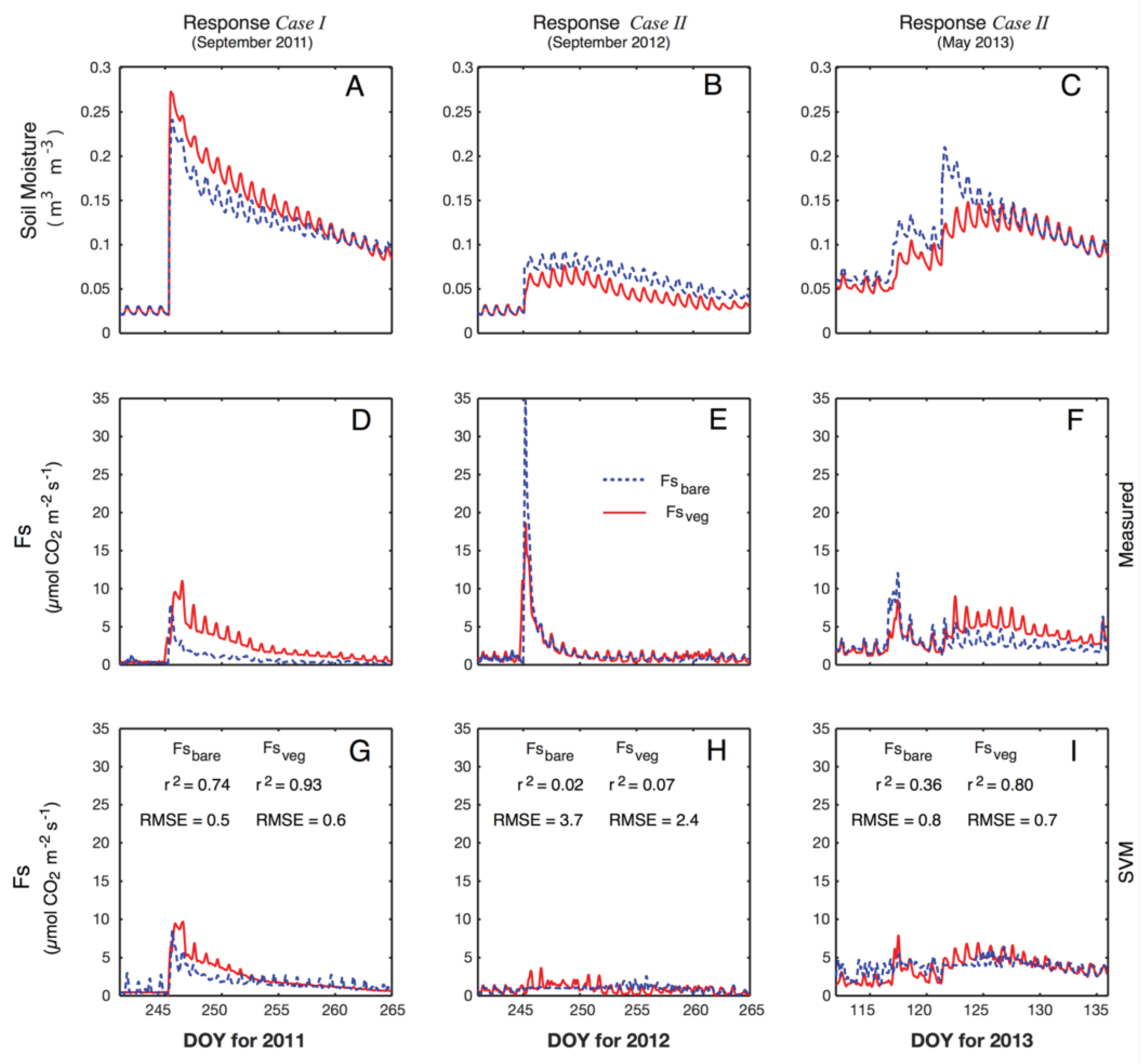
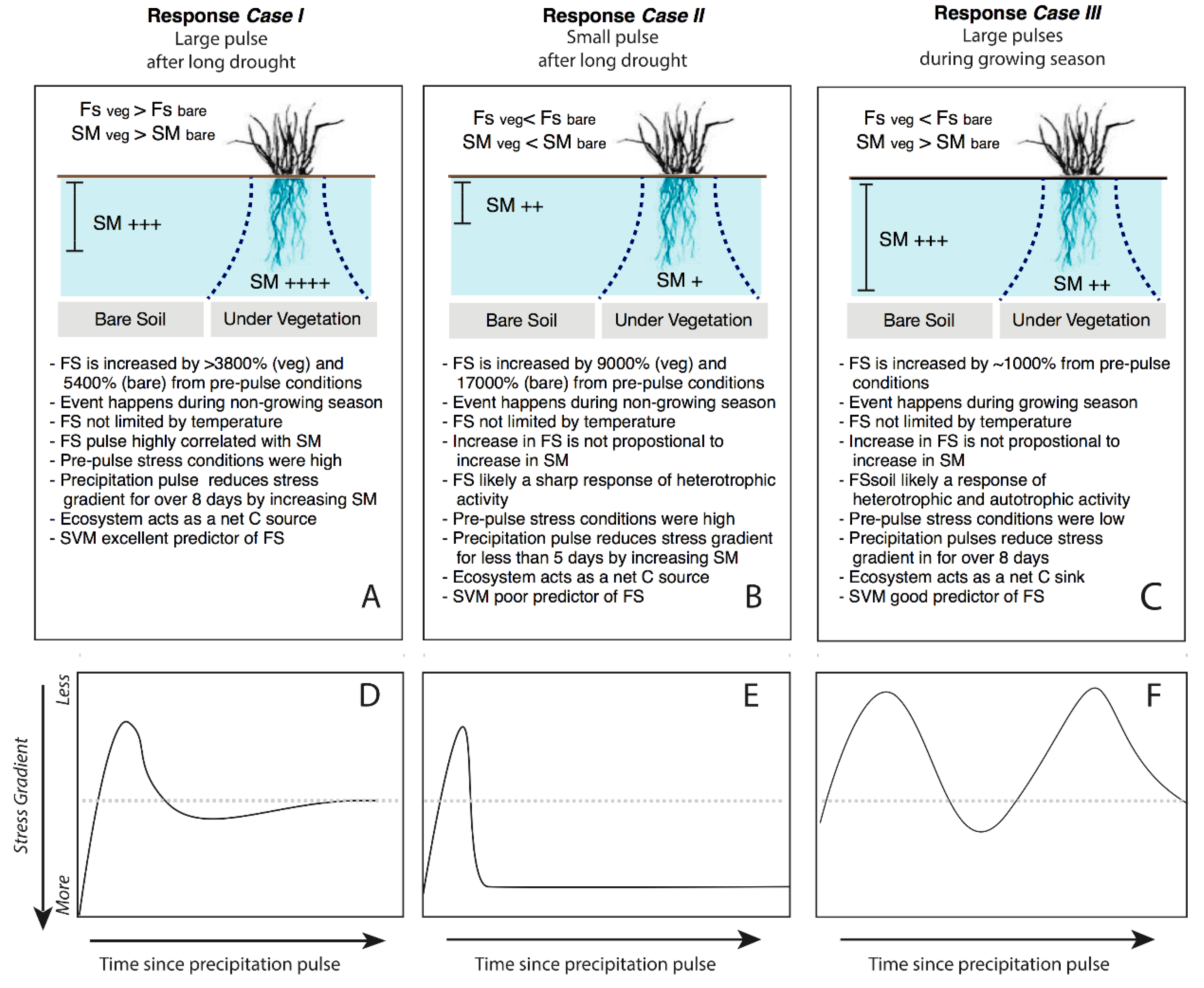
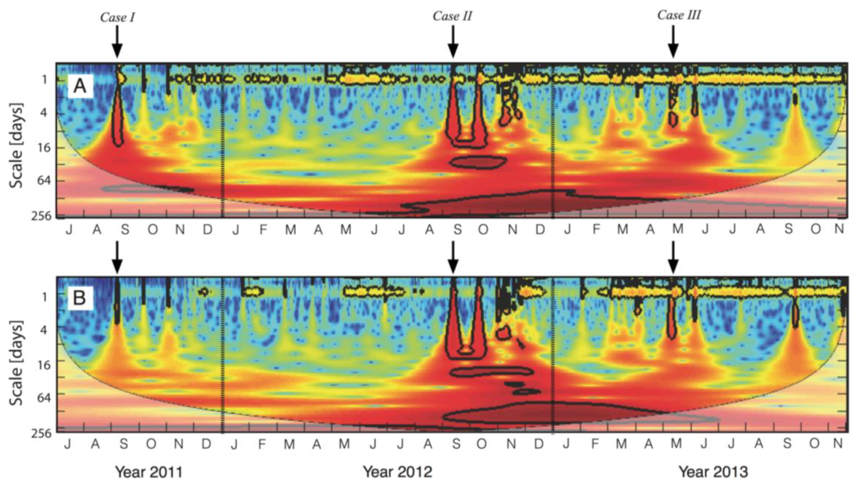
3.4. Responses to Different Precipitation Pulses

We selected three responses (i.e., Cases) to PPs based on the spectral properties of the time series of measurements and model residuals. These response Cases represent rapid discrete changes in the amplitude of soil moisture from a baseline (i.e., pre-pulse conditions), have substantial influence on the spectral properties of the time series (Figure 3), and are difficult to represent by the proposed modeling approaches (Figure 5). We identified that a Case I response was evident during September 2011 (i.e., days of the year 240 to 265), a Case II during September 2012 (i.e., days of the year 240 to 265), and a Case III during March 2013 (i.e., days of the year 110 to 135).

A Case I response followed a large PP (i.e., >20 mm) after the long dry season that sharply increased soil moisture (Figure 7A). This resulted in an increase of Fs_veg to 11.7 µmol CO₂ m⁻² s⁻¹ representing a change of 5400% and of Fs_bare to 8 µmol CO₂ m⁻² s⁻¹ (increase of 3885%) from pre-pulse conditions (Figure 7D). A Case II response followed a small PP (i.e., <5 mm) after the dry season that slightly increased soil moisture (Figure 7E). Despite this modest response in soil moisture Fs_veg increased to 18 µmol CO₂ m⁻² s⁻¹ and Fs_bare to 34.4 µmol CO₂ m⁻² s⁻¹, representing a change of 9000% and 17,000% from pre-pulse conditions, respectively (Figure 7E). A Case III response was a large PP (i.e., >20 mm) during the moist conditions of the growing season that moderately increased soil moisture (Figure 7C) and increased Fs_veg to 8.7 µmol CO₂ m⁻² s⁻¹ and Fs_bare to 11.7 µmol CO₂ m⁻² s⁻¹ representing an increase of 954% and 1099% from pre-pulse conditions, respectively (Figure 7F).

We tested how the three modeling approaches were able to represent the different responses using a 1-h time-step. Overall, all models were able to represent Case I and III responses (Figure S1), but SVM was the model that better represented these responses (Figure 7H, I). None of the models were able to represent a Case II response.

4. Discussion

Our results support the paradigm that the distribution and intensity of PPs influence annual Fs in water-limited ecosystems. Relatively similar total precipitation but lower soil moisture variability resulted in 50% higher Fs emissions during the second hydrologic year. Lower soil moisture variability and prolonged rains (until June 2013) likely reduced water stress during the second hydrologic year. Higher ecosystem metabolic activity during the second year was observed by the consistent periodicity at the 1-day period for Fs_veg and Fs_bare (Figure 3). These results support observations that precipitation patterns which maintain higher soil moisture conditions for a longer time resulted in higher seasonal ecosystem metabolic rates [25,62].

Discrete PPs generate Fs responses that resulted in hot-moments of Fs_veg and Fs_bare (response Case I to III). The wavelet analyses demonstrate that these pulse responses had distinct spectral signatures localized within specific PPs (Figure 3). Not every PP resulted in an event with a distinct spectral signature in the time series of Fs demonstrate the uniqueness of the selected Cases (Figure 3). In other words, despite the fact that there were several PPs throughout the length of the study, we identify three distinct Cases that we interpret as hot-moments of Fs. We recognize that there is a hierarchy of PPs, but we bring attention to the use of time-series analysis and the interpretation of PPs and hot-moments by analyzing information of automated Fs measurements in the frequency-domain. Arguably, previous studies have likely underestimated hot-moments of Fs due to lack of continuous measurements as recent studies are demonstrating the importance of these transient but intense events [29,34,63].

4.1. Can We Model Daily Fs Using Temperature and Soil Moisture Information?

Our results show that the temporal influence of soil moisture on Fs overrides the influence of soil temperature on Fs in this water-limited ecosystem (Figure 4). This supports the fact that temperature is only relevant in these ecosystems when soil moisture is available for metabolic processes [26,35,48]. The temporal influence of soil temperature in this water-limited ecosystem seems to be concentrated at the 1-day period during discrete days when water is available. In contrast, the influence of soil moisture has larger implications for the temporal variability of Fs at scales ranging from 2-to 16-days during the different responses (i.e., Case I to III).

Our results demonstrate the challenge that empirical modeling approaches have to represent hot-moments of Fs in water-limited ecosystems, where a Case II response was consistently challenging to represent by all approaches (Figure 5). A Case II response substantially increased the magnitude of Fs but the magnitude of the response was not proportional to the increase in soil moisture. Although this response is directly linked to an increase in soil moisture, the underlying biotic and abiotic mechanisms go beyond water availability as previously discussed for rewetting events [29,34].

The conditional approach (i.e., Model 1) was able to represent between 47% and 35% of the variability in daily Fs_veg and Fs_bare, respectively. This simple conditional approach can be easily applied across study sites and is interpretable, as it provides insights about temperature and soil moisture sensitivity of Fs (by comparing constants in the model). This approach is widely applicable at the daily-scale and parameters can be compared across sites and across site-years but has the largest uncertainty of all approaches.

The wealth of information from continuous measurements allows for the application of more complex models that can be highly parameterized such as the 8-day moving window approach (i.e., Model 2). This moving window approach follows the fact that water availability and precipitation pulses drive most of the metabolic pulses in this water-limited ecosystem [27]. The use of an 8-day moving window was confirmed by the PWC showing that water pulses have a consistent temporal influence between 8-to 16-days regardless of their magnitude or antecedent moisture conditions. This approach significantly increased the proportion of explained variance to 84% for daily Fs_veg and 48% to daily Fs_bare. This approach could be applied as a gapfilling technique for time series of Fs [64], but has little interpretability and applicability beyond the parameterized time series because parameters are highly variable in order to match measurements for each moving window (Figure 6). Future applications could be done varying the size of the window to optimize for site-specific conditions and to improve gapfilling estimates.

Machine learning approaches are versatile and flexible enough to discover complicated nonlinear relationships and we argue that SVM has the potential for representing the non-stationary dynamics of Fs. This approach was able to increase the representation of daily Fs_bare when compared with the approach of Model 2. Likely the use of more variables has the potential for improvement of predictions of hot-moments of Fs that are controlled by factors beyond soil moisture, but caution must be taken to avoid autocorrelation among variables and model over fitting [65]. The opportunity for machine learning approaches to Fs is arguably starting with a few examples such as the use of random forests [66]; thus, it is expected that the use of these techniques will become more common in the near future.

4.2. How Discrete PPs Influence Hot-Moments of Fs?

We identified three Cases of Fs to PPs where the Fs rate drastically changed (up to 17,000%) to affect the spectral properties of the time series and data-model agreement. Here, we describe the generalities of these responses, but we recognize that our results are based on the information within the available time series and longer records could show consistency or a larger diversity of responses.

Case I represents the ecosystem response after a large PP (>20 mm) following a long drought period, and is characteristic of the beginning of the rainy season in Mediterranean ecosystems [26,27]. Case I is characterized by rapid water infiltration into the soil profile, which substantially increases soil water content in areas of bare soil and under vegetation (Figure 8A). Furthermore, the vegetation could provide a preferential pathway for water infiltration, as demonstrated by an increase of soil moisture with respect to the bare soil. In Case I we observed larger Fs_veg than Fs_bare with two possible explanations. First, we postulate that the autotrophic component of Fs (i.e., Fs_veg minus Fs_bare) increased as plants rapidly start to use resources to activate the photosynthetic mechanism, therefore increasing their catabolism and autotrophic respiration [27]. Second, it is likely that the heterotrophic component of Fs under vegetation has also increased because of higher substrate availability within the rhizosphere that is rapidly dissolved and available for microbes [28]. Notably, the modeling approach by SVM was able to represent this response as Fs was highly correlated with soil moisture regardless of the underlying mechanisms of the heterotrophic and autotrophic components of Fs (Figure 7G).

Case II represents the ecosystem response after a small PP (<5 mm) following a long drought period. This distinction is important because in water-limited ecosystems, the beginning of the rainy season does not always start with a large (i.e., >20 mm) precipitation event [13,67,68]. Case II is characterized by slow water infiltration that only permeates into soil surface layers because it is likely that vegetation intercepts most water from these small PPs and creates a shadow where soil moisture is lower (under vegetation) than at the bare soil (Figures 7B and 8B). Despite the small PP we observed a hot-moment for Fs_veg (18 µmol CO₂ m² s⁻¹) and Fs_bare (>34 µmol CO₂ m² s⁻¹) that increased Fs by 9000 and 17,000% from pre-pulse conditions, respectively. These responses are the highest reported for Fs for rewetting events [29] as a result of very low pre-pulse Fs rates (due to dry conditions during the non-growing season) and the sharp increase following the PP. Previous studies have demonstrated that Fs is spatially heterogeneous within a water-limited ecosystem [26] and that small PPs do not activate the metabolism at the plant-level [27]. We postulate that increases in Fs_veg and Fs_bare are likely driven by an increase in the heterotrophic component of Fs because there is not enough available water to trigger plant catabolic metabolism to stimulate autotrophic respiration (Figure 8B). The lack of correlation between the size of the PP and the response of Fs make modeling of these responses very challenging. None of the proposed approaches were able to represent the response as underlying variables (e.g., available substrate supply) may have influenced the sharp uncorrelated response to soil moisture. The implication of this modeling limitation is that low-to-medium Fs fluxes are usually overrepresented by models and high Fs fluxes are underestimated (Figure 6). Furthermore, these large responses could contribute up to 40% of total net CO₂ emissions during dry seasons [27], so accurate measurements and understanding of these hot-moments is needed to better understand local carbon dynamics.

Case III represents the ecosystem response to a large precipitation event (~20 mm) during the cool and moist growing season (Figure 7C and Figure 8C). We postulate that although the plant canopy can provide a preferential pathway for water infiltration into the soil (as seen in Case I), this season is characterized by less soil moisture limitation and a homogeneous distribution of soil water content across the soil profile (Figure 8C). Case III is characterized by a large change in soil water content with increases in Fs of about 1000%, but this sharp increase only represents <20% of the sharp response observed for Case I and II. Notably, the modeling approach by SVM was able to represent the response of Fs_veg as it was highly correlated with soil moisture, but in a lesser degree the response of Fs_bare which had a disproportionally low response to increased moisture in the soil profile (Figure 7I). We postulate that Case III is likely a result of an increase in heterotrophic and autotrophic activity as plant metabolism is active during the growing season [27].

We borrow the concept of the “bucket model” to describe how discrete PPs influence hot-moments of Fs. The “bucket model” is a conceptual idea to describe the response of terrestrial ecosystems under different precipitation patterns [69]. In this model, the “bucket” represents the uppermost soil layers with maximum root density and is characterized by upper and lower water stress thresholds (i.e., a stress gradient) [69]. We propose that an analogous conceptual approach can be used to explain the hot-moments of Fs in our study. Therefore, “the soil water bucket” represents the uppermost soil layers within maximum root density and is characterized by upper and lower water stress thresholds that represent a gradient of ecosystem stress (Figure 8D–F). In Case I the ecosystem is stressed as a consequence of the long dry season, but the PP is able to increase soil moisture that moves the ecosystem to a state of less stress for a prolonged period of time until the following precipitation event (Figure 8D); this response is highly correlated with the temporal patterns of soil moisture. In Case II the ecosystem is also stressed as a consequence of the long dry season, but soil moisture is not substantially increased, resulting in a short period of reduced stress followed by a sharp return to a previous stressed state (Figure 8E). Finally, in Case III the ecosystem is less stressed and subsequent changes in soil moisture create variability under a stress gradient (Figure 8F). This conceptual idea aims to highlight that variability in PPs defines water-limited ecosystems, pushes these ecosystems towards less-stressed conditions, and could trigger a diverse response of hot-moments of Fs.

Climate models indicate a future with altered precipitation patterns where extreme PPs could be followed by long dry periods in water-limited ecosystems. Thus, it is critical to understand how diverse PPs influence ecosystem processes under different metabolic states. Automated measurements of Fs provide the opportunity to capture high-temporal resolution of ecosystem responses, providing information on disproportionately high (i.e., hot-moments) CO₂ fluxes following precipitation events [34]. Although CO₂ fluxes in water-limited ecosystems are low compared to mesic ecosystems, their sensitivity to changes in precipitation pattern is high and consequently influences their annual net fluxes. Our results support the application of a machine learning approach (i.e., SVM) based on information of soil moisture and temperature to represent Fs, but we recognize that machine learning is parameterized with available data and consequently is not process based. Hot-moments of Fs as a result of a small precipitation event (<5 mm; Case II pulse) following a long drought period appear to be the most challenging events to represent and support the need of continuous measurements to capture the effects of this discrete but sharp response. We demonstrate that soil moisture has high temporal correlation with Fs and overshadows the influence of soil temperature in this water-limited ecosystem. Finally, because the variability of carbon dynamics in water-limited ecosystems influences the global carbon cycle, it is essential to quantify the responses of non-stationary ecosystem CO₂ fluxes to transient (and potentially extreme) precipitation events.

References

1. Poulter, B.; Frank, D.; Ciais, P.; Myneni, R.B.; Andela, N.; Bi, J.; Broquet, G.; Canadell, J.G.; Chevallier, F.; Liu, Y.Y.; et al. Contribution of semi-arid ecosystems to interannual variability of the global carbon cycle. Nature 2014, 509, 600–603. [Google Scholar] [CrossRef] [PubMed]
2. Ahlstrom, A.; Raupach, M.R.; Schurgers, G.; Smith, B.; Arneth, A.; Jung, M.; Reichstein, M.; Canadell, J.G.; Friedlingstein, P.; Jain, A.K.; et al. The dominant role of semi-arid ecosystems in the trend and variability of the land CO2 sink. Science 2015, 348, 895–899. [Google Scholar] [CrossRef] [PubMed]
3. Huxman, T.E.; Smith, M.D.; Fay, P.A.; Knapp, A.K.; Shaw, M.R.; Loik, M.E.; Smith, S.D.; Tissue, D.T.; Zak, J.C.; Weltzin, J.F.; et al. Convergence across biomes to a common rain-use efficiency. Nature 2004, 429, 651–654. [Google Scholar] [CrossRef] [PubMed]
4. Sala, O.E.; Parton, W.J.; Joyce, L.A.; Lauenroth, W.K. Primary production of the central grassland region of the united-states. Ecology 1988, 69, 40–45. [Google Scholar] [CrossRef]
5. Knapp, A.K.; Smith, M.D. Variation among biomes in temporal dynamics of aboveground primary production. Science 2001, 291, 481–484. [Google Scholar] [CrossRef] [PubMed]
6. Noy-Meir, I. Desert ecosystems: Environment and producers. Annu. Rev. Ecol. Syst. 1973, 4, 25–51. [Google Scholar] [CrossRef]
7. Reynolds, J.F.; Kemp, P.R.; Ogle, K.; Fernandez, R.J. Modifying the ‘pulse-reserve’ paradigm for deserts of north america: Precipitation pulses, soil water, and plant responses. Oecologia 2004, 141, 194–210. [Google Scholar] [CrossRef] [PubMed]
8. Huxman, T.E.; Snyder, K.A.; Tissue, D.; Leffler, A.J.; Ogle, K.; Pockman, W.T.; Sandquist, D.R.; Potts, D.L.; Schwinning, S. Precipitation pulses and carbon fluxes in semiarid and arid ecosystems. Oecologia 2004, 141, 254–268. [Google Scholar] [CrossRef] [PubMed]
9. Thomey, M.L.; Collins, S.L.; Vargas, R.; Johnson, J.E.; Brown, R.F.; Natvig, D.O.; Friggens, M.T. Effect of precipitation variability on net primary production and soil respiration in a chihuahuan desert grassland. Glob. Chang. Biol. 2011, 17, 1505–1515. [Google Scholar] [CrossRef]
10. Xu, L. Seasonal variation in carbon dioxide exchange over a mediterranean annual grassland in California. Agric. For. Meteorol. 2004, 123, 79–96. [Google Scholar] [CrossRef]
11. Ogle, K.; Reynolds, J.F. Plant responses to precipitation in desert ecosystems: Integrating functional types, pulses, thresholds, and delays. Oecologia 2004, 141, 282–294. [Google Scholar] [CrossRef] [PubMed]
12. Sala, O.E.; Lauenroth, W.K. Small rainfall events: An ecological role in semi-arid regions. Oecologia 1982, 53, 301–304. [Google Scholar] [CrossRef] [PubMed]
13. Schwinning, S.; Sala, O. Hierarchy of responses to resource pulses in arid and semi-arid ecosystems. Oecologia 2004, 141, 211–220. [Google Scholar] [CrossRef] [PubMed]
14. Curiel Yuste, J.; Baldocchi, D.D.; Gershenson, A.; Goldstein, A.; Misson, L.; Wong, S. Microbial soil respiration and its dependency on carbon inputs, soil temperature and moisture. Glob. Chang. Biol. 2007, 13, 2018–2035. [Google Scholar] [CrossRef] [Green Version]
15. Vargas, R.; Carbone, M.S.; Reichstein, M.; Baldocchi, D.D. Frontiers and challenges in soil respiration research: From measurements to model-data integration. Biogeochemistry 2011, 102, 1–13. [Google Scholar] [CrossRef]
16. Baldocchi, D.; Tang, J.W.; Xu, L.K. How switches and lags in biophysical regulators affect spatial-temporal variation of soil respiration in an oak-grass savanna. J. Geophys. Res. Biogeosci. 2006, 111. [Google Scholar] [CrossRef] [Green Version]
17. Christensen, J.H.; Hewitson, B.; Busuioc, A.; Chen, A.; Gao, X.; Held, R.; Jones, R.; Kolli, R.K.; Kwon, W.K.; Laprise, R.; et al. Regional climate projections, climate change, 2007: The physical science basis. In Contribution of Working Group i to the Fourth Assessment Report of the Intergovernmental Panel on Climate Change; Solomon, S., Qin, D., Manning, M., Chen, Z., Marquis, M., Averyt, K.B., Tignor, M., Miller, H.L., Eds.; University Press: Cambridge, UK, 2007; pp. 847–940. [Google Scholar]
18. Vargas, R.; Collins, S.L.; Thomey, M.L.; Johnson, J.E.; Brown, R.F.; Natvig, D.O.; Friggens, M.T. Precipitation variability and fire influence the temporal dynamics of soil CO2 efflux in an arid grassland. Glob. Chang. Biol. 2012, 18, 1401–1411. [Google Scholar] [CrossRef]
19. Heisler-White, J.L.; Knapp, A.K.; Kelly, E.F. Increasing precipitation event size increases aboveground net primary productivity in a semi-arid grassland. Oecologia 2008, 158, 129–140. [Google Scholar] [CrossRef] [PubMed]
20. Vicca, S.; Bahn, M.; Estiarte, M.; van Loon, E.E.; Vargas, R.; Alberti, G.; Ambus, P.; Arain, M.A.; Beier, C.; Bentley, L.P.; et al. Can current moisture responses predict soil CO2 efflux under altered precipitation regimes? A synthesis of manipulation experiments. Biogeosciences 2014, 11, 2991–3013. [Google Scholar] [CrossRef] [Green Version]
21. Knapp, A.K.; Avolio, M.L.; Beier, C.; Carroll, C.J.; Collins, S.L.; Dukes, J.S.; Fraser, L.H.; Griffin-Nolan, R.J.; Hoover, D.L.; Jentsch, A.; et al. Pushing precipitation to the extremes in distributed experiments: Recommendations for simulating wet and dry years. Glob. Chang. Biol. 2017, 23, 1774–1782. [Google Scholar] [CrossRef] [PubMed]
22. Anderson-Teixeira, K.J.; Delong, J.P.; Fox, A.M.; Brese, D.A.; Litvak, M.E. Differential responses of production and respiration to temperature and moisture drive the carbon balance across a climatic gradient in new mexico. Glob. Chang. Biol. 2011, 17, 410–424. [Google Scholar] [CrossRef]
23. Huxman, T.E.; Cable, J.M.; Ignace, D.D.; Eilts, J.A.; English, N.B.; Weltzin, J.; Williams, D.G. Response of net ecosystem gas exchange to a simulated precipitation pulse in a semi-arid grassland: The role of native versus non-native grasses and soil texture. Oecologia 2004, 141, 295–305. [Google Scholar] [CrossRef] [PubMed]
24. Xu, L.K.; Baldocchi, D.D.; Tang, J.W. How soil moisture, rain pulses, and growth alter the response of ecosystem respiration to temperature. Glob. Biogeochem. Cycles 2004, 18. [Google Scholar] [CrossRef] [Green Version]
25. Jenerette, G.D.; Scott, R.L.; Huxman, T.E. Whole ecosystem metabolic pulses following precipitation events. Funct. Ecol. 2008, 22, 924–930. [Google Scholar] [CrossRef] [Green Version]
26. Leon, E.; Vargas, R.; Bullock, S.H.; Lopez, E.; Panosso, A.R.; La Scala, N. Hot spots, hot moments and spatio-temporal controls on soil CO2 efflux in a water-limited ecosystem. Soil Biol. Biogeochem. 2014, 77, 12–21. [Google Scholar] [CrossRef]
27. López-Ballesteros, A.; Serrano-Ortiz, P.; Sánchez-Cañete, E.v.; Oyonarte, C.; Kowalski, A.S.; Pérez-Priego, Ó.; Domingo, F. Rain pulses enhance the net CO2 release of a semi-arid grassland in se spain. J. Geophys. Res. Biogeosci. 2015. [Google Scholar] [CrossRef]
28. Yan, L.M.; Chen, S.P.; Huang, J.H.; Lin, G.H. Water regulated effects of photosynthetic substrate supply on soil respiration in a semiarid steppe. Glob. Chang. Biol. 2011, 17, 1990–2001. [Google Scholar] [CrossRef]
29. Kim, D.G.; Vargas, R.; Bond-Lamberty, B.; Turetsky, M.R. Effects of soil rewetting and thawing on soil gas fluxes: A review of current literature and suggestions for future research. Biogeosciences 2012, 9, 2459–2483. [Google Scholar] [CrossRef] [Green Version]
30. Ogle, K.; Barber, J.J.; Barron-Gafford, G.A.; Bentley, L.P.; Young, J.M.; Huxman, T.E.; Loik, M.E.; Tissue, D.T. Quantifying ecological memory in plant and ecosystem processes. Ecol. Lett. 2015, 18, 221–235. [Google Scholar] [CrossRef] [PubMed]
31. Potts, D.L.; Huxman, T.E.; Enquist, B.J.; Weltzin, J.F.; Williams, D.G. Resilience and resistance of ecosystem functional response to a precipitation pulse in a semi-arid grassland. J. Ecol. 2006, 94, 23–30. [Google Scholar] [CrossRef] [Green Version]
32. Austin, A.T.; Vivanco, L. Plant litter decomposition in a semi-arid ecosystem controlled by photodegradation. Nature 2006, 442, 555–558. [Google Scholar] [CrossRef] [PubMed]
33. Ma, S.Y.; Baldocchi, D.D.; Hatala, J.A.; Detto, M.; Yuste, J.C. Are rain-induced ecosystem respiration pulses enhanced by legacies of antecedent photodegradation in semi-arid environments? Agric. For. Meteorol. 2012, 154, 203–213. [Google Scholar] [CrossRef]
34. Petrakis, S.; Seyfferth, A.; Kan, J.J.; Inamdar, S.; Vargas, R. Influence of experimental extreme water pulses on greenhouse gas emissions from soils. Biogeochemistry 2017, 133, 147–164. [Google Scholar] [CrossRef]
35. Almagro, M.; Lopez, J.; Querejeta, J.I.; Martinez-Mena, M. Temperature dependence of soil CO2 efflux is strongly modulated by seasonal patterns of moisture availability in a mediterranean ecosystem. Soil Biol. Biochem. 2009, 41, 594–605. [Google Scholar] [CrossRef]
36. Moyano, F.E.; Vasilyeva, N.; Bouckaert, L.; Cook, F.; Craine, J.; Yuste, J.C.; Don, A.; Epron, D.; Formanek, P.; Franzluebbers, A.; et al. The moisture response of soil heterotrophic respiration: Interaction with soil properties. Biogeosciences 2012, 9, 1173–1182. [Google Scholar] [CrossRef] [Green Version]
37. Serrano-Ortiz, P.; Oyonarte, C.; Perez-Priego, O.; Reverter, B.R.; Sanchez-Canete, E.P.; Were, A.; Ucles, O.; Morillas, L.; Domingo, F. Ecological functioning in grass-shrub mediterranean ecosystems measured by eddy covariance. Oecologia 2014, 175, 1005–1017. [Google Scholar] [CrossRef] [PubMed]
38. Aubinet, M.; Grelle, A.; Ibrom, A.; Rannik, U.; Moncrieff, J.; Foken, T.; Kowalski, A.S.; Martin, P.H.; Berbigier, P.; Bernhofer, C.; et al. Estimates of the annual net carbon and water exchange of forests: The euroflux methodology. Adv. Ecol. Res. 2000, 30, 113–175. [Google Scholar]
39. Reichstein, M.; Falge, E.; Baldocchi, D.; Papale, D.; Aubinet, M.; Berbigier, P.; Bernhofer, C.; Buchmann, N.; Gilmanov, T.; Granier, A.; et al. On the separation of net ecosystem exchange into assimilation and ecosystem respiration: Review and improved algorithm. Glob. Chang. Biol. 2005, 11, 1424–1439. [Google Scholar] [CrossRef]
40. Sanchez-Canete, E.P.; Kowalski, A.S. Comment on “using the gradient method to determine soil gas flux: A review” by m. Maier and h. Schack-kirchner. Agric. For. Meteorol. 2014, 197, 254–255. [Google Scholar] [CrossRef]
41. Puigdefabregas, J.; Sole, A.; Gutierrez, L.; del Barrio, G.; Boer, M. Scales and processes of water and sediment redistribution in drylands: Results from the rambla honda field site in southeast spain. Earth-Sci. Rev. 1999, 48, 39–70. [Google Scholar] [CrossRef]
42. Oyonarte, C.; Rey, A.; Raimundo, J.; Miralles, I.; Escribano, P. The use of soil respiration as an ecological indicator in arid ecosystems of the se of spain: Spatial variability and controlling factors. Ecol. Indic. 2012, 14, 40–49. [Google Scholar] [CrossRef]
43. Rey, A.; Pegoraro, E.; Oyonarte, C.; Were, A.; Escribano, P.; Raimundo, J. Impact of land degradation on soil respiration in a steppe (Stipa tenacissima L.) semi-arid ecosystem in the se of spain. Soil Biol. Biochem. 2011, 43, 393–403. [Google Scholar] [CrossRef]
44. Fan, J.; Jones, S.B. Soil surface wetting effects on gradient-based estimates of soil carbon dioxide efflux. Vadose Zone J. 2014, 13. [Google Scholar] [CrossRef]
45. Jones, H.G. Plants and Microclimate: A Quantitative Approach to Environmental Plant Physiology; Cambridge University Press: New York, NY, USA, 1992; p. 51. [Google Scholar]
46. Moldrup, P.; Olesen, T.; Schjonning, P.; Yamaguchi, T.; Rolston, D.E. Predicting the gas diffusion coefficient in undisturbed soil from soil water characteristics. Soil Sci. Soc. Am. J. 2000, 64, 94–100. [Google Scholar] [CrossRef]
47. Vargas, R.; Allen, M.F. Dynamics of fine root, fungal rhizomorphs, and soil respiration in a mixed temperate forest: Integrating sensors and observations. Vadose Zone J. 2008, 7, 1055–1064. [Google Scholar] [CrossRef]
48. Barron-Gafford, G.A.; Scott, R.L.; Jenerette, G.D.; Huxman, T.E. The relative controls of temperature, soil moisture, and plant functional group on soil CO2 efflux at diel, seasonal, and annual scales. J. Geophys. Res. 2011, 116. [Google Scholar] [CrossRef]
49. Burges, C.J.C. A tutorial on support vector machines for pattern recognition. Data Min. Knowl. Discov. 1998, 2, 121–167. [Google Scholar] [CrossRef]
50. Smola, A.J.; Scholkopf, B. A tutorial on support vector regression. Stat. Comput. 2004, 14, 199–222. [Google Scholar] [CrossRef] [Green Version]
51. Rasmussen, C.E.; Williams, C.K.I. Gaussian Processes for Machine Learning; Adaptive Computation and Machine Learning Series; The MIT Press: Cambridge, MA, USA, 2005; pp. 1–247. [Google Scholar]
52. Keerthi, S.S.; Lin, C.J. Asymptotic behaviors of support vector machines with gaussian kernel. Neural Comput. 2003, 15, 1667–1689. [Google Scholar] [CrossRef] [PubMed]
53. Torrence, C.; Compo, G.P. A practical guide to wavelet analysis. Bull. Am. Meteorol. Soc. 1998, 79, 61–78. [Google Scholar] [CrossRef]
54. Vargas, R.; Baldocchi, D.D.; Bahn, M.; Hanson, P.J.; Hosman, K.P.; Kulmala, L.; Pumpanen, J.; Yang, B. On the multi-temporal correlation between photosynthesis and soil co2 efflux: Reconciling lags and observations. New Phytol. 2011, 191, 1006–1017. [Google Scholar] [CrossRef] [PubMed]
55. Ding, R.; Kang, S.; Vargas, R.; Zhang, Y.; Hao, X. Multiscale spectral analysis of temporal variability in evapotranspiration over irrigated cropland in an arid region. Agric. Water Manag. 2013, 130, 79–89. [Google Scholar] [CrossRef]
56. Katul, G.; Lai, C.T.; Schafer, K.; Vidakovic, B.; Albertson, J.; Ellsworth, D.; Oren, R. Multiscale analysis of vegetation surface fluxes: From seconds to years. Adv. Water Resour. 2001, 24, 1119–1132. [Google Scholar] [CrossRef]
57. Vargas, R.; Detto, M.; Baldocchi, D.D.; Allen, M.F. Multiscale analysis of temporal variability of soil CO2 production as influenced by weather and vegetation. Glob. Chang. Biol. 2010, 16, 1589–1605. [Google Scholar] [CrossRef]
58. Dietze, M.C.; Vargas, R.; Richardson, A.D.; Stoy, P.C.; Barr, A.G.; Anderson, R.S.; Arain, M.A.; Baker, I.T.; Black, T.A.; Chen, J.M.; et al. Characterizing the performance of ecosystem models across time scales: A spectral analysis of the north american carbon program site-level synthesis. J. Geophys. Res. Biogeosci. 2011, 116. [Google Scholar] [CrossRef]
59. Stoy, P.C.; Dietze, M.C.; Richardson, A.D.; Vargas, R.; Barr, A.G.; Anderson, R.S.; Arain, M.A.; Baker, I.T.; Black, T.A.; Chen, J.M.; et al. Evaluating the agreement between measurements and models of net ecosystem exchange at different times and timescales using wavelet coherence: An example using data from the north american carbon program site-level interim synthesis. Biogeosciences 2013, 10, 6893–6909. [Google Scholar] [CrossRef] [Green Version]
60. Grinsted, A.; Moore, J.C.; Jevrejeva, S. Application of the cross wavelet transform and wavelet coherence to geophysical time series. Nonlinear Process. Geophys. 2004, 11, 561–566. [Google Scholar] [CrossRef] [Green Version]
61. Ng, E.K.W.; Chan, J.C.L. Geophysical applications of partial wavelet coherence and multiple wavelet coherence. J. Atmos. Ocean. Technol. 2012, 29, 1845–1853. [Google Scholar] [CrossRef]
62. Scott, R.L.; Serrano-Ortiz, P.; Doming, F.; Hamerlynck, E.P.; Kowalski, A.S. Commonalities of carbon dioxide exchange in semiarid regions with monsoon and mediterranean climates. J. Arid Environ. 2012, 84, 71–79. [Google Scholar] [CrossRef]
63. Phillips, C.L.; Bond-Lamberty, B.; Desai, A.R.; Lavoie, M.; Risk, D.; Tang, J.W.; Todd-Brown, K.; Vargas, R. The value of soil respiration measurements for interpreting and modeling terrestrial carbon cycling. Plant Soil 2017, 413, 1–25. [Google Scholar] [CrossRef]
64. Gomez-Casanovas, N.; Anderson-Teixeira, K.; Zeri, M.; Bernacchi, C.J.; DeLucia, E.H. Gap filling strategies and error in estimating annual soil respiration. Glob. Chang. Biol. 2013, 19, 1941–1952. [Google Scholar] [CrossRef] [PubMed]
65. Thiessen, U.; van Brakel, R.; de Weijer, A.P.; Melssen, W.J.; Buydens, L.M.C. Using support vector machines for time series prediction. Chemom. Intell. Lab. Syst. 2003, 69, 35–49. [Google Scholar] [CrossRef]
66. Bond-Lamberty, B.; Bunn, A.G.; Thomson, A.M. Multi-year lags between forest browning and soil respiration at high northern latitudes. PLoS ONE 2012, 7, e50441. [Google Scholar] [CrossRef] [PubMed]
67. Rey, A.; Oyonarte, C.; Moran-Lopez, T.; Raimundo, J.; Pegoraro, E. Changes in soil moisture predict soil carbon losses upon rewetting in a perennial semiarid steppe in se spain. Geoderma 2017, 287, 135–146. [Google Scholar] [CrossRef]
68. Cleverly, J.; Boulain, N.; Villalobos-Vega, R.; Grant, N.; Faux, R.; Wood, C.; Cook, P.G.; Yu, Q.; Leigh, A.; Eamus, D. Dynamics of component carbon fluxes in a semi-arid acacia woodland, central australia. J. Res. Biogeosci. 2013, 118, 1168–1185. [Google Scholar] [CrossRef]
69. Knapp, A.K.; Beier, C.; Briske, D.D.; Classen, A.T.; Luo, Y.; Reichstein, M.; Smith, M.D.; Smith, S.D.; Bell, J.E.; Fay, P.A.; et al. Consequences of more extreme precipitation regimes for terrestrial ecosystems. Bioscience 2008, 58, 811–821. [Google Scholar] [CrossRef]
Figure 1. Time series of daily mean of soil temperature (A), daily sum of precipitation, daily mean of soil moisture (B), daily mean of soil CO2 efflux (Fs) nearby vegetation (Fsveg) and in bare soil (Fsbare; C), and daily mean of net ecosystem exchange (NEE; D). Dashed lines in panels A–C represent variables measured under vegetation and solid lines represent variables measured in bare soil. Gray areas in panels B and C represent precipitation pulses selected as response cases (i.e., Case I, Case II, Case III; see results section). Solid circles in panel B represent precipitation. Letters in the x-axis represents months of the year from July 2011 to November 2013.
Soilsystems 02 00047 g001
Figure 2. Time series of half-hour values of soil CO2 efflux under vegetation (Fsveg; A) and in bare soil (Fsbare; B). Letters in the x-axis represents months of the year from July 2011 to November 2013; y-axis represent each hour of the day.
Soilsystems 02 00047 g002
Figure 3. Continuous wavelet power spectra using the continuous wavelet transform of the time series of soil respiration under vegetation (Fsveg; A) and in bare soil (Fsbare; B). The color codes for power values are from yellow (low values) to dark red (high values). Black contour lines represent the 5% significance level and thin black line indicates the cone of influence that delimits the region not influenced by edge effects. Letters in the x-axis represents months of the year from July 2011 to November 2013. Arrows represent “hot-moments” of Fs identified for this study.
Soilsystems 02 00047 g003
Figure 4. Partial wavelet coherence analysis (PWC) to test the influence of soil temperature (controlling for soil moisture) on soil CO2 efflux in areas under vegetation (Fsveg; A) or in bare soil (Fsbare; B). PWC analysis to test the influence of soil moisture (controlling for soil temperature) on CO2 efflux in areas under vegetation (Fsveg; C) or in bare soil (Fsbare; D). The color codes for temporal correlation are from blue (low values) to yellow (high values). Yellow areas within black contour lines represent the 5% significance level for power values (i.e., high temporal correlation); the thin black line indicates the cone of influence that delimits the region not influenced by edge effects. Gray areas in panels C and D represent precipitation pulses analyzed to characterize the response cases (i.e., Case I, Case II, Case III). Letters in the x-axis represents months of the year from July 2011 to November 2013.
Soilsystems 02 00047 g004
Figure 5. Analysis of model residuals of soil CO2 efflux (Fs) under vegetation (Fsveg; AF) or in bare soil (Fsbare; GL). Residuals using Equations (2) and (3) (Model 1), Support Vector Machine (SVM) or an 8-day window approach (Model 2) for Fsveg (A,C,E) and Fsbare (G,I,K). Continuous wavelet power spectra using the continuous wavelet transform for residuals of each model for Fsveg (B,D,F) and Fsbare (H,J,L). The color codes for power values are from yellow (high values) to red (low values). Yellow areas within black contour lines represent the 5% significance level for power values (i.e., high value of residuals); the thin black line indicates the cone of influence that delimits the region not influenced by edge effects.
Soilsystems 02 00047 g005
Figure 6. Probability density functions of soil CO2 efflux (Fs) values for measurements and each model under vegetation (Fsveg; A) and bare soil (Fsbare; C). Cumulative sums of soil CO2 fluxes for measurements and each model under vegetation (Fsveg; B) and bare soil (Fsbare; D). Letters in the x-axis represents months of the year from July 2011 to November 2013. For a description of the models see methods section. SVM = support vector machine.
Soilsystems 02 00047 g006
Figure 7. Pulse responses of soil moisture (AC), Fs under vegetation (Fsveg) or in bare soil (Fsbare; DF), and model output using support vector machine (SVM) for Fsveg or Fsbare (GI). Responses are defined as Case I-III, and are identified in Figure 1 and Figure 3. Solid lines represent variables measured under vegetation and dashed lines represent variables measured in bare soil. Fs means soil CO2 efflux. The numbers in the x-axis represent the day of the year (DOY) for years 2011 to 2013 for each panel.
Soilsystems 02 00047 g007
Figure 8. Summary of selected Fs responses to precipitation pulses (AC), and conceptual depiction of the contingent responses of the ecosystem to precipitation pulses (DF). The rectangles in D–F represent a “soil water bucket”, where the “y” axis represents a stress gradient and the dotted line represents a reference point for comparison among panels. Selected responses are defined as Case I–III, and are identified in Figure 1, Figure 3 and Figure 7. Case I results in less stressful conditions for several days, Case II is characterized by a short period of stress relief, and Case III is in between fluctuations of less water stress. Fsveg = soil CO2 efflux in areas under vegetation; Fsbare = soil CO2 from areas without vegetation (i.e., bare soil); SM = soil moisture, where the number of “+” signs denotes higher soil moisture either at bare soil or under vegetation.
Soilsystems 02 00047 g008