
Acid Gas Re-Injection System Design Using Machine Learning


1
School of Mining and Metallurgical Engineering, National Technical University of Athens, 15780 Athens, Greece
2
Institute of Geoenergy, Foundation for Research and Technology-Hellas, 73100 Chania, Greece
*
Author to whom correspondence should be addressed.
Clean Technol. 2022, 4(4), 1001-1019; https://doi.org/10.3390/cleantechnol4040062
Submission received: 23 June 2022
/
Revised: 22 August 2022
/
Accepted: 9 October 2022
/
Published: 13 October 2022
Abstract
:An “energy evolution” is necessary to manifest an environmentally sustainable world while meeting global energy requirements, with natural gas being the most suitable transition fuel. Covering the ever-increasing demand requires exploiting lower value sour gas accumulations, which involves an acid gas treatment issue due to the greenhouse gas nature and toxicity of its constituents. Successful design of the process requires avoiding the formation of acid gas vapor which, in turn, requires time-consuming and complex phase behavior calculations to be repeated over the whole operating range. In this work, we propose classification models from the Machine Learning field, able to rapidly identify the problematic vapor/liquid encounters, as a tool to accelerate phase behavior calculations. To set up this model, a big number of acid gas instances are generated by perturbing pressure, temperature, and acid gas composition and offline solving the stability problem. The generated data are introduced to various classification models, selected based on their ability to provide rapid answers when trained. Results show that by integrating the resulting trained model into the gas reinjection process simulator, the simulation process is substantially accelerated, indicating that the proposed methodology can be readily utilized in all kinds of acid gas flow simulations.
1. Introduction
Undoubtedly, the ever-growing global energy demand in conjunction with the immaturity of carbon free energy sources has forwarded natural gas as the transition fuel [1,2] until the net zero task [3] is accomplished. As a result, gas hydrocarbon reservoirs, which have been traditionally ignored due to limited quality of their organic content, are now considered as potential candidates. A typical example of such reservoirs is those containing CO2 and H2S rich fluids which, in turn, leads to the production of sour surface gas streams. Primary to its transportation and market release, the sour gas must undergo a process of selectively removing the acid components, i.e., H2S and CO2, due to the high toxicity of the former [4] as well as the corrosive nature and direct impact on the increase of the greenhouse effect [5,6] of the latter. This separation process, known as gas sweetening, takes place in the amine unit (AU) and results in an acid-free sweet gas stream and a second waste acid gas stream, which is extremely flammable and explosive, containing significant amounts of H2S and CO2. In order to protect the environment from toxic and greenhouse gases, the aforementioned waste stream must be handled properly.
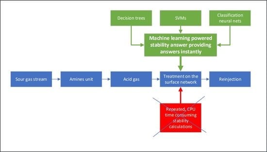
Typically, the waste acid gas stream is driven into a Claus Sulfur Recovery (CSR) unit, where elemental sulfur from gaseous H2S is recovered [7,8,9,10]. However, due to declining global demand for elemental sulfur [11] as well as increasingly stringent emission standards [12], alternative ways of handling the acid gas are sought after, with the most straightforward application being the stream injection into the reservoir [13]. This process is illustrated in Figure 1 and can be described by the following steps. Firstly, the fluids collected from all wellheads contributing to production are flowed to a separator where complete liquid–gas separation occurs at predetermined pressure and temperature conditions [14]. The resulting sour gas stream is then led to a drying unit where most of the water content is removed [15]. Subsequently, this dried sour gas is directed towards the AU plant where, in contact with an amine solution, an absorption process enables the sweet components to pass through, while maintaining the acid components in the water phase [16,17]. Ultimately, conforming to pipeline and market specifications for low acid gas content [18], the sweet gas is driven to the sales point. The remaining acid gas-saturated amine solvent is regenerated by heating the aqueous solution and the water-saturated acid gas stream exits the regenerator unit at 35 to 70 kPa to be subsequently cooled and compressed at suitable pressure stages [19]. Finally, the acid gas stream is driven through pipelines to the wellheads [13] where it is injected selectively back to the reservoir.
The study and development of an acid gas injection scheme requires thorough estimation of the fluid’s complex phase equilibria [13,20]. However, literature provides limited experimental data as far as the phase behavior and the physical properties of acid gas mixtures are concerned [21,22,23,24]. Therefore, the phase behavior and physical properties must be evaluated using computational models with conditions varying in a very wide range, from near-atmospheric ones, to those prevailing at the surface processing plant and transportation network, and eventually to those encountered in the wellbore and the reservoir. Additionally, the phases encountered at each stage of the reinjection process also vary between those of gas, liquid, and supercritical at the AU outlet, the transportation network, and the wellbore respectively. For the latter case, the acid gas must be injected at a supercritical state to ensure high density and lack of gas bubbles, which could lead to severe erosion and to the prevention of adverse permeability effects [20,23]. On top of the above concerns, the compositional variability of the injected gas stream, as influenced by the production planning of the field, must be further considered. This is due to the commingling of fluids originating from different parts of the reservoir which contain diverse fluids with respect to their acid components concentration [25].
To study the acid gas stream flow from the AU outlet to the reservoir, the differential equations accounting for the conservation of mass, momentum and energy need to be solved. Commonly, pipelines and wellbores are discretized into 1D elements within which the conservation equations are converted to sets of algebraic equations and solved iteratively. The number and properties of the flowing phases need to be determined at each discretization block, for all iterations until convergence, and for every time step [26]. To attack this problem in compositional simulation, the standard method to answer the phase state question is running a phase stability test which determines the number of phases present in the flowing fluid at the prevailing pressure and temperature conditions [27,28,29], i.e., whether it lies inside or outside the phase envelope, as shown in Figure 2. Although the algorithm is straightforward, a highly non-linear optimization problem needs to be solved to get the number of phases, which imposes a big CPU time burden on the total simulation time cost. This is due to the iterative nature of the optimization problem as well as the implemented EoS model, the cost of which may vary between as low as that of a conventional cubic EoS model, to as high as that of much more complex models such as the Cubic Plus Association (CPA) [30,31]. Since speed is a critical concern in current compositional flow simulators, accelerating stability calculations without too much compromise in accuracy and reliability is an active research topic in both academia and industry [32,33,34].
In the Machine Learning (ML) context, classification is a process that assigns a given object (pattern) to a class (target, label, or category) [35]. In its simplest case, the classification problem is binary with the assigned class being on/off, high/low etc., although multiclass problems can be handled as well. During its training against a dataset, the classifier learns the classes decision boundary using ML algorithms, which aim at minimizing the misclassification error [36]. This dataset is referred to as a training dataset and includes several samples, as well as the desired class for each sample from which to learn, in what is known as a supervised learning scheme. The decision boundary is often a parametric expression of the input features, and the optimal values of the parameters are obtained through the training process. The classifier’s efficiency to correctly map input data to a specific category is evaluated based on its ability to classify previously “unseen” test data, which have not been utilized throughout the training process. Special attention should be paid to the classifier’s complexity as it must be adjusted to optimize model’s generalization capability and to avoid obtaining overtrained complex models which may exhibit flawless classification results on the training set, but not on new data (overfitting) [37]. Therefore, the tradeoff between a highly complicated structure that is prone to overfitting and a simplistic structure that produces poor classification results on novel observation samples (underfitting) must be optimized.
Clearly, the phase stability problem can be mapped to a two-class classification—one with the two classes corresponding to stable/unstable or equivalently to single/two-phase flow. Therefore, ML classification techniques can be used to generate accurate and rapid predictions regarding the number of phases present of various acid gas instances. The input features are the acid gas composition, , pressure, , and temperature, [38]. The exact phase boundaries in the p-T phase diagrams represent the decision boundaries that need to be learned and accurately reproduced by the classifier (Figure 2). Once such a machine has been trained, it can be directly incorporated to the flow simulator, fully replacing the conventional, iterative, time-consuming stability algorithm, thus offering significant acceleration of the flow simulation time cost.
Various applications of similar proxy modeling have appeared in the literature. Such models have been developed by means of soft computing tools, varying from classic statistical methods to high end ML approaches. Water-Alternating-Gas procedures and the Box–Behnken design have been optimized by means of such methods to establish Enhanced Recovery [39,40,41]. Moreover, full scale reservoir simulation of hydrocarbon recovery or CO2 injection for storage purposes have also been drastically accelerated by means of proxy modeling using neural networks [42,43]. Similarly, proxy modeling by means of ML has been applied to accelerate turbulent multiphase flow simulations [44], whereas vast acceleration of condensate gas reservoir simulation has been reported [45]. Fault detection in complex NGL fractionation processes has also been treated [46].
In this paper, we investigate the applicability of ML techniques in handling the phase behavior classification, with the purpose of dealing more efficiently with the complexity and computational cost of phase equilibrium calculations in acid gas flow simulation. Various classification models from the ML field have been tested to come up with the optimal architecture, which combines optimal error rate and fast predictions on new data.
The paper is laid out as follows: Section 2 discusses all materials and methods utilized in this work, including conventional stability algorithm and CPU time needs when complex Equation of State (EoS) models are utilized, how phase stability can be mapped to a classification problem, and sets forth the classification techniques used in the paper consisting of Decision Trees (DTs), Support Vector Machines (SVMs), and Neural Network (NN)-based classifiers as investigated candidates. Section 3 describes how the training data were generated, explains all data treatment techniques employed, and discusses the results obtained for each classification model, as well as the special techniques utilized to further accelerate computations. Conclusions are presented in Section 4.
2. Materials and Methods
2.1. Conventional Stability Calculations
Phase stability testing is an integral part of the phase behavior calculations required in all multiphase flow simulations. The conventional approach is based on the work of Michelsen [28], who developed the Tangent Plane Distance (TPD) criterion [29]. According to Michelsen’s criterion, a mixture will split into two or more phases if a composition can be found, which leads to a reduction of the mixture’s Gibbs energy when an infinitesimal quantity of that composition forms a second phase (a bubble or a drop). The Gibbs energy of a -component mixture of composition , at given temperature and pressure , is computed by [32,47]
where the chemical potential of component at current conditions. If an infinitesimal amount of a new phase, , forms a second phase with composition , then the change in Gibbs energy will be
the sign of which equals that of the TPD function:
If a composition can be found which reduces the system’s Gibbs energy, the system will switch to a two-phase system and acid gas vapor will coexist with liquid. To avoid searching the full compositional space, only composition that minimizes can alternatively be considered. On the other hand, if , i.e., , the system will remain in the single phase. Therefore, Michelsen’s criterion states that [32]
where
Stability analysis is formulated as a nonlinear, unconstrained minimization problem that aims at locating the stationary points of the TPD function where its derivative vanishes. To avoid convergence to trivial solutions, at least two different initial estimates of composition need to be tried [32]. Minimization is run using any conventional algorithm from simple Successive Substitution Iteration to the highly sophisticated Newton method. Global minimization of the TPD might also be sought, depending on the complexity of the TPD function, as is done in the work by McDonald and Floudas [48], Harding and Floudas [49], and Hua et al. [50,51]. Although global minimization methods are reliable and guaranteed to arrive at the global minimum of the TPD function for a suitable initial guess, they are also costly and limited to systems with a small number of components.
Computational speed is a severe issue when dealing with multiple stability calculations as is the case for flow simulation. The problem stems from the fact that the EoS which governs acid gas thermodynamics needs to be solved repeatedly for each trial composition to get the system’s Gibbs energy reduction , hence and its gradient. A large number of studies have been presented which aim at accelerating such computations, including lumping of the reservoir fluid composition into a smaller number of pseudo-components [52] while preserving the EoS model’s accuracy as much as possible. Reduction methods were initiated by Michelsen [53], who was the first to link the number of non-linear equations that need to be solved in phase-split calculations to the rank of the binary interaction coefficients matrix (BIC). He showed that in the extreme case of zero BIC, the system equations are only three, on the condition that the Van der Waals mixing rules are utilized. Hendricks and Van Bergen [54], Firoozabadi and Pan [55], and Pan and Firoozabadi [56] extended this idea to phase stability calculations and to fluids with non-zero BIC. By applying singular value decomposition to the BIC matrix and by maintaining only its dominant directions, the original variables are replaced by a set of new ones with , thus significantly reducing the dimensionality of both problems.
2.2. Stability Calculations in the Classification Framework
Classification aims at assigning a label to an object judging from its description by a set of measured features. In its simplest version, the labeling is binary as each object is assigned to one of two classes, say true and false or high and low [35]. To build the classifier, a training dataset is required, comprising of a set of instances, usually obtained by an experimental procedure, for which a set of features is available for each instance together with the required label. The classifier training procedure aims at generating an expression, which mathematically combines the features values to arrive at the correct label output.
If a classifier is trained to predict the probability of each class to be the correct one, e.g., and then datapoint is assigned to class A if . Alternatively, classifiers can be trained to generate an appropriate discriminating function for which and . Therefore, to label a new point the discriminating function is evaluated and the appropriate class is assigned according to its sign.
Gaganis and Varotsis [32,57,58] utilized the classification framework to allow the rapid run of batch stability computations. They proposed the use of data-driven classifiers which would directly assign a stable/unstable label to any operating conditions. More specifically, they developed discriminating functions of the form exhibiting same sign with over the full operating range. Such a function will provide same stability predictions as the conventional criterion; hence the stability state of a mixture would be determined by [32]
where the third branch corresponds to the phase boundary.
In this work, we utilize datapoints describing the acid gas thermodynamic behavior to generate an explicit expression of the function. Let a set of data points , where denotes combinations of composition, pressure, and temperature and takes values in with corresponding to a stable and corresponding to an unstable mixture respectively. Such a set can be constructed beforehand by utilizing any reliable stability algorithm for an arbitrarily large random set of inputs fully covering the required simulation , , and space. The discriminating function is generated to satisfy and for all data points, that is, providing positive or negative values for stable and unstable points, respectively. If satisfies that constraint for all datapoints contained in the sampled dataset, it will also correctly interpolate the discriminating function sign (0 or 1) for any other possible combination of composition, pressure, and temperature, thus providing a correct stability answer in the entire required operating range. Once has been developed, the stability state for any acid gas mixture can be declared rapidly by means of Equation (6). By generating against data obtained from thermodynamically consistent methods, Equation (6) can be thought of as an equivalent non-iterative, closed form solution of the formal stability problem in Equations (3)–(5).
The explicitness of Equation (6) allows for the computation of the stability state directly, in a non-iterative mode and in a fraction of the CPU time required by the conventional, iterative approaches. Therefore, during a flow simulation run, Equation (6) can fully replace the conventional stability test at any iteration of the non-linear solver for each grid block and at any time step. Furthermore, the proposed method can be utilized with an EoS model of any complexity and with any set of mixing rules. By completely avoiding time-consuming iterations and the requirement for suitable initial estimates, the number of operations required for any test case is constant even in the vicinity of the critical point, the stability test limit locus [59], and the supercritical region [32].
2.3. Classification Models Considered
The classification problem studied in this work exhibits certain peculiarities compared to the vast majority of similar problems appearing in the data science field. Firstly, an arbitrarily large amount of training data can be readily generated off-line as a closed form method to get the class of any composition, i.e., conventional stability calculation, available. Therefore, overfitting can be avoided as the ratio between the training population size and the classification model parameters space can be controlled. Secondly, it is important to keep the model size and the computational load as low as possible to guarantee rapid answers to the stability problem at any point along the fluids path and at any operating conditions. As a result, various classification models available in the literature which may exhibit remarkable accuracy levels may not be applicable to the problem studied here.
The selection of suitable classification models is initially approached by setting up the problem on a rigid mathematical basis. More specifically, let be the training data matrix which contains the input of datapoints, each consisting of features, also known as response variables. In the present case, each row corresponds to a single datapoint with columns for fluid composition, pressure, and temperature, i.e., where stands for the number of acid gas components. The corresponding labels for each case are stored in a vector which comprises unities and zeros, representative of each state, i.e., stable or unstable, respectively. The classifier generates a discriminating function where and its training aims at modifying to minimize the discrepancy between exact and predicted labels, usually defined by means of negative likelihood, piecewise linear cost, cross entropy, and the negative Gini index [37].
Based on the features of the problem under study, three classification models were investigated: DTs, SVMs, and classification NNs. DTs build classification models in the form of a tree by applying continuous division of the input space into halfplanes according to response variables and threshold values which define the division point. The training algorithm repeatedly selects the response variable and the threshold value which, when applied to the training population, leads to its optimal split. Optimality can be determined by means of various criteria, with the most pronounced one being the Gini index [37], which accounts for the similarity of the points assigned to each split. The Gini index exhibits maximum value when all cases belonging to a single split exhibit same class labels which in turn implies that further splitting and growing of the tree is not required and that the particular node is a terminating one. The training CPU time cost of this category of classifier is very low and so is the prediction time on future datapoints, as decisions are obtained by applying simple and uncostly if commands. Additionally, a low number of split levels adds to the bias of the model while reducing its variance, thus improving the bias/variance tradeoff and preventing overfitting [60].
SVMs [61,62] aim at generating a discriminating function of the form which exhibits opposite signed values on points belonging to the two classes. The discriminating function equals to zero exactly at the boundary between the two classes and SVMs aim at positioning the boundary to maximize its distance between the closest datapoints of the two classes, known as margin. For any input , the discriminating function is a linear combination of regressors which are non-linear on the response variables, usually by means of kernel functions between the input and the training datapoints collected in matrix . As a result, a SVM is driven by a model of the form
SVM training aims at adjusting model’s unknown parameters and to maximize the margin, that is, the distance between the boundary and its adjacent datapoints [63]. Mathematically, this corresponds to a constrained quadratic optimization problem which is convex, thus guaranteeing a single global minimum, but still requires iterative calculations due to the linear constraints which are as many as the training datapoints. Matrix in Equation (7) only needs to contain those training datapoints with a non-zero weight , known as Support Vectors (SVs). As obtaining new predictions costs as much as the evaluation of , to ensure rapid predictions, simple kernel functions need to be utilized in conjunction to as few as possible SVs obtained by the training procedure.
Classification NNs [64] are conventional back propagation neural networks, equipped with a softmax function at the output node. They can be thought of as machines which firstly combine the input features to a non-linear mapping at the hidden layer and subsequently combine linearly the latter to arrive at the model output. For the present case of a binary output, the softmax function simplifies to the classic logistic function. Therefore, any network output below 0.5 corresponds to the first class, whereas values above that threshold imply that the datapoint corresponds to the second class. For a model of inputs and hidden neurons, the model output is given by
and the classification label is given by
To minimize the impact on a quadratic least-squares cost function of those points lying away from the discriminating function, the negative likelihood cost function is preferred, defined by
which needs to be minimized in terms of the variables vector that contains all models tunable parameters . Clearly, minimizing needs to be run iteratively which leads to a time-consuming training procedure, sensitive to the initial estimates of .
3. Results and Discussion
3.1. Generation of the Training Data
The training dataset utilized in this work consists of a large number of pairs , where and composition vector contains the concentration of all four components typically found in acid gas mixtures, that is CO2, H2S, C1, and C2. The input vectors were randomly drawn from a uniform distribution so that they densely cover the anticipated range of reservoir and surface conditions of the acid gas re-injection system. The requirement that valid composition mole fractions sum up to unity implies that should be sampled from the dimension simplex to avoid linear dependence of the inputs, thus reducing the input vector size to 5. The corresponding stable/unstable assignments are obtained by utilizing any conventional stability algorithm. The generated dataset can be arbitrarily large and the data are noise-free, as they are generated by a thermodynamically consistent method such as Michelsen’s algorithm [32].
As the most important components involved in acid gas re-injection operations are H2S and CO2, with C1 and C2 being light hydrocarbon impurities, compositions were randomly drawn from the uniform distribution shown in Table 1. The lower pressure limit was dictated by the acid gas output pressure from the AU, which is close to the atmospheric one. Although the upper limit can be arbitrarily high, it was set at 1500 psi since acid gas is always in single state, liquid or supercritical, for any given composition and temperature above that pressure [65]. Similarly, the temperature lower limit was set to 39.2° F (4 °C) to account for the minimum possible subsea temperature and the upper limit was set at 220° F, which is the maximum at which two phase equilibrium may appear [65].
As the acid gas phase envelopes only occupy a limited part of the p-T range, uniformly drawn data points lying close to the phase boundary, which are critical to the generation of the discriminating function, are significantly less that those spread around in the operating space. To enhance their population, each randomly generated point was assigned to the suitable pool depending on its location. Subsequently, datapoints were drawn from both pools at user-controlled ratios to form the training population. To determine whether a random datapoint lies close to the phase envelope or not, four additional points were generated enclosing the point under investigation, as shown in Figure 3, exhibiting pressure or temperature difference of 50 psi or 5 °F, respectively. If all five neighboring points exhibit the same stability result (either stable or unstable), then the point lies away from the boundary, whereas if the stability results of any pair of neighboring points differ then the datapoint under investigation lies near to the phase boundary.
To further accelerate computations, the operating space that needs to be checked for two-phase equilibrium was significantly reduced by applying simple p-T bounds, defined to optimally enclose the instability area, given by simple quadratic functions of temperature. Those functions allow the rapid determination of acid gas stability state for the vast majority of the conditions under question. As can be seen in Figure 4, if the prevailing p-T conditions lie above the black or below the grey limiting lines, they explicitly correspond to a single-phase mixture, thus relieving the need to utilize the trained classifier. This way, a rapid response can be obtained for about two-thirds of all possible p-T conditions. Summarizing, the selection procedure is based on the following rules:
- Acid gas is explicitly stable at temperatures above the highest cricodentherm and at pressures above the highest cricodenbar, 1500 psi and 220 °F, respectively;
- Acid gas is explicitly stable if current conditions lie above the upper boundary line;
- Acid gas is explicitly stable if current conditions lie below the lower boundary line;
- Otherwise, the classifier needs to be invoked to identify the number of phases present at current operating conditions.
The commercial software used in this work is MATLAB, and all codes were setup using commands offered by the Statistics and Machine Learning Toolbox.
3.2. Classifiers Training
3.2.1. Decision Trees
In this work, DTs based on node splitting by means of the Gini index were selected as a classifier model on the basis of the limited dimensionality of the input vector. To reduce the risk of building overfitted models, the training population size was increased to 5 million datapoints, with two-thirds of them accounting for points lying close to the boundary. Similarly, the maximum number of splits was allowed to vary between a very modest value of only 100 splits up to as high as 20,000. Note that even for such high numbers of splits, the CPU time cost to obtain predictions can be quite low, as the number of if commands required to realize the tree scales with the logarithm of the number of the splits.
The resulting model exhibited remarkable accuracy against the training data implying that the multidimensional step function developed by the DT successfully discriminates stable from unstable points. This is demonstrated by the confusion matrix shown in Table 2, with the model performance resulting in 1.93% false stable and 1.19% false unstable predictions, respectively, out of the total population. Correspondingly, false stable and false unstable predictions account for 8.59% and 1.54% of all stable and unstable points, respectively. To evaluate the model performance on new unseen points, 5000 testing datapoints of various p-T conditions, sharing a fixed sample composition of an H2S rich mixture, were generated (10%, 86%, 2%, 2% of CO2, H2S, C1, and C2). This time, the confusion matrix of the testing dataset indicates wrong answers for 2.46% and 1.40% of the total population, which implies uniform model accuracy against both training and testing data.
However, a more thorough examination of the results reveals severe issues, suggesting high variance of the trained model. As shown in Figure 5, correctly labeled points are shown in green, whereas red and blue indicates misclassified points lying either inside or outside the true phase envelope. Clearly, the plot shows many misclassified points, stable or unstable ones, thus imposing the danger of severe errors in the flow simulation. In fact, as long as the erroneous predictions lie close to the phase boundary, the error introduced to the flow simulation is minor. Indeed, if an unstable mixture close to the phase boundary is erroneously predicted to be stable, the flow simulator will only miss a very small amount of gas (or liquid), which will only have a minor effect on the simulation. If a stable acid gas mixture is predicted to be unstable this poses no problem to the solution accuracy, except for the CPU cost of an unnecessary extra phase split algorithm, which will prove that a second phase does not really exist. In the present case, although most of the misclassifications lie close to the phase boundary, others still lie either deep inside the phase envelope or far away from it, corresponding to cases of severe classification error. Such errors indicate poor bias–variance tradeoff and poor generalization properties of the trained DT [60].
As far as the number of nodes is concerned, developing as many as 20,000 nodes sounds like a huge tree which may need a long CPU time to provide predictions on new data. Given the number of if commands required to arrive at a terminating node scale with the base-2 logarithm due to the binary nature of each node, that number of nodes corresponds to a maximum of 15 decisions before arriving to a concrete decision. To further evaluate the prediction time cost, the number of if commands required for all training data points was computed, and its cumulative histogram is shown in Figure 6. It can be readily seen that predictions for 56% of the data points can be obtained at a cost of 8 if commands, 92% of them can be labeled in 11 commands at most, and 98% with 12 commands, with each if command utilizing the original features rather than some complex transformation of them.
The high DTs variance is a well-known problem in the field which has traditionally been treated by means of bagging or boosting [35]. In the case studied in this work, tree bagging was tested to generate random forests, and the results obtained were significantly enhanced, with the misclassification error been reduced down to less than 0.2% and all erroneous answers lying very close to the phase boundary. However, the price to be paid was a large number of trees being grown to a moderate depth. A random forest comprising of 100 trees, each 200 nodes deep, was found to exhibit excellent performance, but the total CPU cost became unaffordable, thus leading to dropping random forests as an option for the acid gas mixtures’ stability problem.
3.2.2. Support Vector Machines
SVMs equipped with a suitable kernel function were also tested. As the training data is noiseless, the machine is guaranteed to correctly classify all training data, provided that it is equipped with a kernel function of sufficient complexity, potentially at the cost of a big number of SVs. However, bearing in mind that developing models which respond rapidly to new data during flow calculations are of utmost importance, the introduction of slack, also known as box constraint, was required. This way, the model was allowed to misclassify a few points lying close to the decision boundary to keep the number of SVs low. The SV population can also be indirectly controlled by keeping the size low of the training population at the potential cost of increased misclassification rate. For the kernel function, the pronounced choice is that of a polynomial kernel as the phase envelope of all acid gas mixtures on the p-T plane correspond to closed curves, as shown in Figure 2.
Various combinations of training dataset size, kernel function selection, and slack values were tried to identify the model that exhibits maximum accuracy while using minimum number of SVs, hence exhibiting minimum complexity. Our trials indicated that introducing approximately 5000 labeled training datapoints with a polynomial kernel function of the 4th degree, i.e., and moderate slack values of the order of 10, provide optimal results with the number of SV’s arriving to 713 and misclassifications only appearing very close to the phase boundary. The number of SVs, and consequently, the complexity of the SVM implementing formula, can be further reduced by applying a model reducing procedure like the one originally presented by Burges et al. [66].
The model performance on the training data resulted in only 1.72% and to 0.92% false stable and false unstable predictions, respectively according to Table 3. Those figures correspond to significantly better rates compared to the DT solution, although they were generated on a much smaller, yet representative, training set. For another 5000 testing datapoints drawn uniformly in the p-T space and combined constantly to the acid gas composition described in the previous section, the rates obtained were only 0.56% and 0.96%, thus demonstrating the improved generalization capability of the SVMs.
The misclassifications obtained on the testing dataset are shown in Figure 7, with red color indicating false unstable and blue color indicating false stable answers. The results verify that wrong answers only lie close to the phase boundary, where the effect of such mistakes to the flow simulation is negligible.
3.2.3. Neural Networks
As discussed in Section 2.3, the NN classifiers utilized in this work are simple feed-forward models with a single hidden layer and a logistic function applied at the single output node. Therefore, model complexity is controlled by the number of hidden neurons. The transformation of the input vector to a new feature vector at the hidden layer offered great flexibility to the model and allowed it to adapt to the true underlying discriminating function that successfully separates points in the training dataset. However, as it contributes to the non-linearity of the cost function and to the danger that the training procedure gets trapped to a poor local optimum, the model training had to be repeated a great number of times.
The simplest ANN model that produced solely minor misclassifications was comprised of 16 hidden neurons, thus implying that the and weight matrices were of size 16 × 5 and 1 × 16, respectively. Therefore, a very modest cost of 17 exponential calls (each in a single sigmoid function evaluation) is needed to arrive at a label prediction for any new datapoint. Despite its reduced size, the ANN performed far better than any other machine tried, as the misclassification rate for false stable and unstable points arrived at 0.85% for both sets (Table 4). Moreover, by examining the results obtained on the fixed acid gas mixture composition, each and every misclassified point was verified to lie very close to the phase boundary, as shown in Figure 8. The error rate for composition was 0.12% and 0.22% for the false stable and unstable points, leading to a total misclassification rate of 0.34%. Similar performance was observed for a CO2 rich composition, namely 80%, 15%, 3%, 2% of CO2, H2S, C1, and C2 as far as both the misclassification locations are concerned, as shown in Figure 9, as well as their rate, which was only 0.36%.
3.3. Further Calculations Speed-Up
To further speed up predictions on new mixtures, a divide-and-conquer approach was attempted by splitting the operating domain into smaller, distinct regions and building a separate model for each region [67]. The reduced size of each model’s operating space also drastically reduces the size and the training time of the model itself. In this work, the overall operating space was split along the and axes into non-overlapping regions of equal size, and a separate classifier was developed for each region (Figure 10).
To obtain the phase state on any new point, one needs to determine the suitable classifier according to the prevailing p and T values and run it to get a prediction. The additional cost required to identify the proper prediction model is negligible, as the regions are equally spaced, and the formulae to define the suitable split for a random pair are given by
where the operator denotes the integer part. Interestingly, all points in the highest temperature and lowest pressure region (i.e., ) were proved to be stable, thus relieving the need to train a model for that particular region. The number of hidden neurons required to achieve descent accuracy for each submodel was significantly reduced and eventually was found to vary between 6 and 7, as opposed to the dimensionality of the unique ANN model which needed 16 neurons, thus reducing the CPU time cost to get an answer to almost half of that of the big model. The exact size of each model is shown in Table 5.
The size of the training and testing datasets for each classification model are summarized in Table 6. Please note that testing points utilized during training to avoid overfitting have only been used during the development of the neural networks. On the other hand, the reported validation datasets were used to optimize the models’ hyper-parameters (such as number of splits and number of hidden nodes).
4. Conclusions
New solutions are required in humanity’s endeavor to handle the current climate change crisis while ensuring sufficient global energy supply. Although natural gas is part of the solution due to the limited competence of the renewable energy sources, acid gas often appears as a byproduct which needs to be treated due to its environmental and health impact. For that purpose, operation of acid gas reservoirs involves gas reinjection, a flow procedure which is commonly simulated by means of extremely time-consuming phase equilibria calculations, among them binary stability calculations. In this work, classification models from the ML field such as DTs, SVMs, and classification NNs were introduced in an attempt to drastically reduce calculation time at minor or even no loss of accuracy.
It was shown that the generated dataset covering the pressure, temperature, and composition ranges encountered in an acid gas reservoir and surface facilities is noiseless and well defined, thus allowing for good training results. Among the classification models examined, NNs exhibited by far the best performance with the lowest total misclassification rate of the testing data, and misclassifications practically located on the phase boundary, thus having an insubstantial effect on the flow simulation. The CPU time cost to get a stability prediction using the developed classifiers was shown to be orders of magnitude less than that of a conventional, iterative stability calculation. Finally, it was shown that calculations can be further accelerated by limiting the operating space between the p-T boundaries, which optimally enclose the instability area, and by further splitting the operating range in subdomains with a separate, low size model built for each region.
Concluding, ML was shown to act as the perfect method to generate proxy models to accelerate stability calculations in acid gas flow simulations. This way, the process engineers will be able to run more complex scenarios and offer a more detailed, more versatile, and less expensive system design.
Author Contributions
Conceptualization, A.S. and V.G.; methodology, A.S. and V.A.; software, V.A. and A.S.; validation, V.G.; resources, R.K.; writing—original draft preparation, A.S. and R.K.; writing—review and editing, V.A. and V.G.; visualization, A.S. All authors have read and agreed to the published version of the manuscript.
Funding
This research received no external funding.
Institutional Review Board Statement
Not applicable.
Informed Consent Statement
Not applicable.
Conflicts of Interest
The authors declare no conflict of interest.
References
- Smil, V. Natural Gas: Fuel for the 21st Century; Wiley: Hoboken, NJ, USA, 2015; ISBN 978-1-119-01286-3. [Google Scholar]
- Stephenson, E.; Doukas, A.; Shaw, K. Greenwashing gas: Might a ‘transition fuel’ label legitimize carbon-intensive natural gas development? Energy Policy 2012, 46, 452–459. [Google Scholar] [CrossRef]
- European Council. Paris Agreement on Climate Change. Available online: http://www.consilium.europa.eu/en/policies/climate-change/timeline/ (accessed on 3 September 2019).
- Eylander, J.G.R.; Holtman, H.A.; Salma, T.; Yuan, M.; Callaway, M.; Johnstone, J.R. The Development of Low-Sour Gas Reserves Utilizing Direct-Injection Liquid Hydrogen Sulphide Scavengers. In Proceedings of the SPE Annual Technical Conference and Exhibition, New Orleans, LA, USA, 30 September–3 October 2001; p. SPE-71541-MS. [Google Scholar]
- Luqman, A.; Moosavi, A. The Impact of CO2 Injection for EOR & its Breakthrough on Corrosion and Integrity of New and Existing Facilities. In Proceedings of the Abu Dhabi International Petroleum Exhibition & Conference, Abu Dhabi, United Arab Emirates, 7–10 November 2016. [Google Scholar]
- Anderson, T.R.; Hawkins, E.; Jones, P.D. CO2, the greenhouse effect and global warming: From the pioneering work of Arrhenius and Callendar to today’s Earth System Models. Endeavour 2016, 40, 178–187. [Google Scholar] [CrossRef] [PubMed] [Green Version]
- Kohl, A.L.; Nielsen, R.B. Gas Purification, 5th ed.; Gulf Professional Publishing: Houston, TX, USA, 1997; pp. 670–730. ISBN 9780884152200. [Google Scholar]
- Kokal, S.L.; Abdulwahid, A. Sulfur Disposal by Acid Gas Injection: A Road Map and A Feasibility Study. In Proceedings of the SPE Middle East Oil and Gas Show and Conference, Al Manama, Bahrain, 12–15 March 2005; p. SPE-93387-MS. [Google Scholar]
- Goar, B. Sulfur Recovery Technology. Energy Progress 1986, 6, 71–75. [Google Scholar]
- Scott, B.; (Bruce Scott, Inc., San Rafael, CA, USA); Hendricks, D.; (Pacific Environmental Services, Inc., Research Triangle Park, NC, USA). Personal communication, 28 February 1992.
- Bachu, S.; Adams, J.J.; Michael, K.; Buschkuehle, B.E. Acid Gas Injection in the Alberta Basin: A Commercial-Scale Analogue for CO2 Geological Sequestration in Sedimentary Basins. In Proceedings of the Second Annual Conference on Carbon Dioxide Sequestration, Alexandria, VA, USA, 5–8 May 2003. [Google Scholar]
- Clark, M.A.; Svrcek, W.Y.; Monnery, W.O.; Jamaluddin, A.K.M.; Bennion, D.B.; Thomas, F.B.; Wichert, E.; Reed, A.E.; Johnson, D.J. Designing and Optimized Injection Strategy for Acid Gas Disposal without Dehydration. In Proceedings of the 77th Annual Convention of the Gas Processors Association, Dallas, TX, USA, 16–18 March 1998. [Google Scholar]
- Carroll, J.J.; Maddocks, J.R. Design considerations for acid gas injection. In Proceedings of the 49th Laurance Reid Gas Conditioning Conference, Norman, OK, USA, 21–24 February 1999. [Google Scholar]
- Powers, M.L. New Perspective on Oil and Gas Separator Performance. SPE Prod. Facil. 1993, 8, 77–83. [Google Scholar] [CrossRef]
- Aitani, A.M. Sour Natural Gas Drying. Hydrocarbon Process. 1993, 72, 67–73. [Google Scholar]
- Speight, J.G. Oil and Gas Corrosion Prevention, 1st ed.; Gulf Professional Publishing: Houston, TX, USA, 2014; pp. 3–37. ISBN 9780128004159. [Google Scholar]
- Weiland, R.H.; Sivasubramanian, M.S.; Dingman, J.C. Effective Amine Technology: Controlling Selectivity, Increasing Slip, and Reducing Sulfur. In Proceedings of the 53rd Annual Laurance Reid Gas Conditioning Conference, Norman, OK, USA, 24 February 2003. [Google Scholar]
- Lens, P.; Hulshoff, P.L.W. Environmental Technologies to Treat Sulfur Pollution: Principles and Engineering, 1st ed.; IWA Publishing: London, UK, 2000; pp. 238–239. ISBN 13: 9781900222099. [Google Scholar]
- Tsang, C.F.; Apps, J.A. Underground Injection Science and Technology, 1st ed.; Elsevier Science: Amsterdam, The Netherlands, 2005; p. 624. ISBN 9780080457901. [Google Scholar]
- Ng, H.; Carroll, J.J.; Maddocks, J. Impact of Thermophysical Properties Research on Acid Gas Injection Process Design. In Proceedings of the 78th Annual GPA Convention, Nashville, TN, USA, 1–3 March 1999. [Google Scholar]
- Bierlein, J.A.; Kay, W.B. Phase-Equilibrium Properties of System Carbon Dioxide-Hydrogen Sulfide. Ind. Eng. Chem. 1953, 45, 618–624. [Google Scholar]
- Kellerman, S.; Stouffer, C.; Eubank, P.; Holste, J.; Hall, K.; Gammon, B.; Marsh, K. Thermodynamic Properties of CO2 + H2S Mixtures; Gas Processors Association: Tulsa, OK, USA, 1995; OCLC: 37647473. [Google Scholar]
- Bennion, D.; Thomas, F.; Schulmeister, B.; Imer, D.; Shtepani, E. The Phase Behavior of Acid Disposal Gases and the Potential Adverse Impact on Injection or Disposal Operations. In Proceedings of the Petroleum Society’s Canadian International Petroleum Conference, Calgary, AB, Canada, 11–13 June 2002. [Google Scholar]
- Commodore, J.A.; Deering, C.E.; Bernard, F.; Marriott, R.A. High-Pressure Densities and Excess Molar Volumes for the Binary Mixture of Carbon Dioxide and Hydrogen Sulfide at T = 343–397 K. J. Chem. Eng. Data 2021, 66, 4236–4247. [Google Scholar] [CrossRef]
- Ahmed, T. Reservoir Engineering Handbook, 4th ed.; Elsevier: Amsterdam, The Netherlands, 2010; ISBN 9780080966670. [Google Scholar]
- Ezekwe, N. Petroleum Reservoir Engineering Practice; Pearson Education: Westford, MA, USA, 2010; ISBN 9780132485210. [Google Scholar]
- Baker, L.E.; Pierce, A.C.; Luks, K.D. Gibbs Energy Analysis of Phase Equilibria. SPE J. 1982, 22, 731–742. [Google Scholar] [CrossRef]
- Michelsen, M.L. The isothermal flash problem: Part I. Stability. Fluid Phase Equilibria 1982, 9, 1–19. [Google Scholar] [CrossRef]
- Michelsen, M.L. The isothermal flash problem. Part II. Phase-split calculation. Fluid Phase Equilibria 1982, 9, 21–40. [Google Scholar] [CrossRef]
- Kontogeorgis, G.M.; Voutsas, E.; Yakoumis, I.; Tassios, D.P. An equation of state for associating fluids. Ind. Eng. Chem. Res. 1996, 35, 4310–4318. [Google Scholar] [CrossRef]
- Tsivintzelis, I.; Kontogeorgis, G.; Michelsen, M.; Stenby, E. Modeling phase equilibria for acid gas mixtures using the CPA equation of state. Part II: Binary mixtures with CO2. Fluid Phase Equilibria 2011, 306, 38–56. [Google Scholar] [CrossRef]
- Gaganis, V.; Varotsis, N. Machine learning methods to speed up compositional reservoir simulation. In Proceedings of the SPE Europec/EAGE Annual Conference, Copenhagen, Denmark, 4–7 June 2012; p. SPE-154505-MS. [Google Scholar]
- Nichita, D.V.; Petitfrere, M. Phase stability analysis using a reduction method. Fluid Phase Equilibria 2013, 358, 27–39. [Google Scholar] [CrossRef]
- Li, Y.; Zhang, T.; Sun, S. Acceleration of the NVT-flash calculation for multicomponent mixtures using deep neural network models. Ind. Eng. Chem. Res. 2019, 58, 12312–12322. [Google Scholar] [CrossRef] [Green Version]
- Bishop, C.M. Pattern Recognition and Machine Learning, 1st ed.; Springer: New York, NY, USA, 2006; ISBN 10: 978-0-387-31073-2. [Google Scholar]
- Nocedal, J.; Wright, S. Numerical Optimization, 2nd ed.; Mikosch, T.V., Robinson, S.M., Resnick, S.I., Eds.; Springer: New York, NY, USA, 2006; ISBN 0-387-30303-0. [Google Scholar]
- James, G.; Witten, D.; Hastie, T.; Tibshirani, R. An Introduction to Statistical Learning: With Applications in R; Springer: New York, NY, USA, 2013; ISBN 978-1-4614-7139-4. [Google Scholar]
- Gaganis, V. Rapid phase stability calculations in fluid flow simulation using simple discriminating functions. Comput. Chem. Eng. 2018, 108, 112–127. [Google Scholar] [CrossRef]
- Amara, M.; Ghahfarokhi, A.; Wui, C.; Zeraibi, N. Optimization of WAG in real geological field using rigorous soft computing techniques and nature-inspired algorithms. J. Pet. Sci. Eng. 2021, 206, 109038. [Google Scholar] [CrossRef]
- Amara, M.; Zeraibi, N.; Redouane, K. Optimization of WAG Process Using Dynamic Proxy, Genetic Algorithm and Ant Colony Optimization. Arab. J. Sci. Eng. 2018, 43, 6399–6412. [Google Scholar] [CrossRef]
- Ahmadi, M.; Zendehboudi, S.; James, L. Developing a robust proxy model of CO2 injection: Coupling Box–Behnken design and a connectionist method. Fuel 2018, 215, 904–914. [Google Scholar] [CrossRef]
- Amini, S.; Mohaghegh, S. Application of Machine Learning and Artificial Intelligence in Proxy Modeling for Fluid Flow in Porous Media. Fluids 2019, 4, 126. [Google Scholar] [CrossRef] [Green Version]
- Shahkarami, A.; Mohaghegh, S. Applications of smart proxies for subsurface modelling. Pet. Explor. Dev. 2020, 47, 400–412. [Google Scholar] [CrossRef]
- Ganti, H.; Kamin, M.; Khare, P. Design Space Exploration of Turbulent Multiphase Flows Using Machine Learning-Based Surrogate Model. Energies 2020, 13, 4565. [Google Scholar] [CrossRef]
- Samnioti, A.; Anastasiadou, V.; Gaganis, V. Application of Machine Learning to Accelerate Gas Condensate Reservoir Simulation. Clean Technol. 2022, 4, 153–173. [Google Scholar] [CrossRef]
- Usama, A.; Daegeun, H.; Jinjoo, A.; Umer, Z.; Chonghun, H. Fault propagation path estimation in NGL fractionation process using principal component analysis. Chemom. Intell. Lab. Syst. 2017, 162, 72–82. [Google Scholar]
- Petitfrere, M. EOS Based Simulations of Thermal and Compositional Flows in Porous Media. Ph.D. Thesis, University of Pau and Pays de l’Adour, Pau, France, 12 September 2014. [Google Scholar]
- McDonald, C.M.; Floudas, C.A. Global optimization for the phase stability problem. AIChE J. 1995, 41, 1798–1814. [Google Scholar] [CrossRef]
- Harding, S.T.; Floudas, C.A. Phase stability with cubic equations of state: A global optimization approach. AIChE J. 2000, 46, 1422–1440. [Google Scholar] [CrossRef]
- Hua, J.Z.; Brennecke, J.F.; Stadtherr, M.A. Reliable prediction of phase stability using an interval Newton method. Fluid Phase Equilibria 1996, 116, 52–59. [Google Scholar] [CrossRef] [Green Version]
- Hua, J.Z.; Brennecke, J.F.; Stadtherr, M.A. Reliable computation of phase stability using interval analysis: Cubic equation of state models. Comput. Chem. Eng. 1998, 22, 1207–1214. [Google Scholar] [CrossRef]
- Whitson, C.; Brule, M. Phase Behavior, SPE Monograph; Henry, L., Ed.; Doherty Memorial Fund of AIME, Society of Petroleum Engineers: Richardson, TX, USA, 2000. [Google Scholar]
- Michelsen, M.L. Simplified flash calculations for cubic equations of state. Ind. Eng. Chem. Process Des. Dev. 1986, 25, 184–188. [Google Scholar] [CrossRef]
- Hendricks, E.M.; Van Bergen, A.R.D. Application of a reduction method to phase equilibria calculations. Fluid Phase Equilibria 1992, 74, 17–34. [Google Scholar] [CrossRef]
- Firoozabadi, A.; Pan, H. Fast and robust algorithm for the compositional modeling: Part I. Stability analysis testing. SPE J. 2002, 7, 78–89. [Google Scholar] [CrossRef] [Green Version]
- Pan, H.; Firoozabadi, A. Fast and robust algorithm for compositional modeling: Part II—Two-phase flash computations. SPE J. 2003, 8, 380–391. [Google Scholar] [CrossRef]
- Gaganis, V.; Varotsis, N. Non-iterative phase stability calculations for process simulation using discriminating functions. Fluid Phase Equilibria 2011, 314, 69–77. [Google Scholar] [CrossRef]
- Gaganis, V.; Varotsis, N. An integrated approach for rapid phase behavior calculations in compositional modeling. J. Petrol. Sci. Eng. 2014, 118, 74–87. [Google Scholar] [CrossRef]
- Nichita, D.V.; Broseta, D.; Montel, F. Calculation of convergence pressure/temperature and stability test limit loci of mixtures with cubic equations of state. Fluid Phase Equilibria 2007, 261, 176–184. [Google Scholar] [CrossRef]
- Hastie, T.; Tibshirani, R.; Friedman, J. The Elements of Statistical Learning: Data Mining, Inference, and Prediction, 2nd ed.; Springer: New York, NY, USA, 2009; ISBN 10: 0387952845. [Google Scholar]
- Burges, C. A tutorial on Support Vector Machines for pattern recognition. Data Min. Knowl. Discov. 1998, 2, 121–167. [Google Scholar] [CrossRef]
- Cortes, C.; Vapnik, V. Support vector networks. Mach. Learn. 1995, 20, 273–297. [Google Scholar]
- Platt, J.C. Fast training of support vector machines using Sequential Minimum Optimization, advances in kernel methods. In Support Vector Machines; MIT Press: Cambridge, MA, USA, 1999; pp. 185–208. [Google Scholar]
- Bishop, C.M. Neural Networks for Pattern Recognition; Oxford University Press: New York, NY, USA, 1995; ISBN 978-0-19-853864-6. [Google Scholar]
- Carroll, J.J. Phase Equilibria Relevant to Acid Gas Injection, Part 1-Non-Aqueous Phase Behavior. J. Can. Pet. Technol. 2002, 41, PETSOC-02-06-02. [Google Scholar]
- Burges, C. Simplified support vector decision rules. In Proceedings of the 13th International Conference on Machine Learning, Bari, Italy, 3–6 July 1996. [Google Scholar]
- Gordon, V.S.; Crouson, J. Self-Splitting Modular Neural Network—Domain Partitioning at Boundaries of Trained Regions. In Proceedings of the IEEE International Joint Conference on Neural Networks, Hong Kong, China, 1–8 June 2008. [Google Scholar]
Figure 1.
Acid gas treatment and reinjection process.

Figure 2.
Phase envelopes for acid gas mixtures.

Figure 3.
Procedure to pick points close to the phase boundary.

Figure 4.
Simple boundaries.

Figure 5.
Visualization of the decision tree model results on testing datapoints.

Figure 6.
Cumulative number of “if” commands required to arrive to a definite answer.

Figure 7.
Visualization of the SVM model results on testing datapoints.

Figure 8.
Visualization of the neural network model results on testing datapoints (86% H2S).

Figure 9.
Visualization of the neural network model results on testing datapoints (80% CO2).

Figure 10.
Visualization of the 3 × 3 split neural network model results on testing datapoints (86% H2S).
Figure 10.
Visualization of the 3 × 3 split neural network model results on testing datapoints (86% H2S).


Table 1.
Range of acid gas mixture components concentration.
| Component | Range (mol%) |
|---|---|
| CO2 | 1–99% |
| H2S | 1–99% |
| C1 | 0–5% |
| C2 | 0–3% |
Table 2.
DT confusion matrices on training and testing data.
| Training Data | Testing Data | ||||||
|---|---|---|---|---|---|---|---|
| True labels | True labels | ||||||
| Stable | Unstable | Stable | Unstable | ||||
| Classifier labels | Stable | 20.52% | 1.19% | Classifier labels | Stable | 28.90% | 1.40% |
| Unstable | 1.93% | 76.36% | Unstable | 2.46% | 67.24% | ||
Table 3.
SVM confusion matrices on training and testing data.
| Training Data | Testing Data | ||||||
|---|---|---|---|---|---|---|---|
| True labels | True labels | ||||||
| Stable | Unstable | Stable | Unstable | ||||
| Classifier labels | Stable | 31.16% | 0.92% | Classifier labels | Stable | 30.32% | 0.96% |
| Unstable | 1.72% | 66.20% | Unstable | 0.56% | 68.16% | ||
Table 4.
ANN confusion matrices on training and testing data.
| Training Data | Testing Data | ||||||
|---|---|---|---|---|---|---|---|
| True labels | True labels | ||||||
| Stable | Unstable | Stable | Unstable | ||||
| Classifier labels | Stable | 28.09% | 0.85% | Classifier labels | Stable | 14.62% | 0.22% |
| Unstable | 0.85% | 70.21% | Unstable | 0.12% | 85.04% | ||
Table 5.
Number of hidden neurons in each submodel.
| P | ||||
|---|---|---|---|---|
| Low (1) | Medium (2) | High (3) | ||
| T | Low (1) | 6 | 7 | 6 |
| Medium (2) | 7 | 7 | 6 | |
| High (3) | - | 6 | 6 | |
Table 6.
Training, testing, and validation datasets.
| Classification Model | Training Datapoints | Validation Datapoints |
|---|---|---|
| Decision trees | 5,000,000 | 1,000,000 |
| Support Vector Machines | 5000 | 5000 |
| Neural networks | 5000 | 5000 |
| 3 × 3 split neural networks | 5000 | 5000 |
Publisher’s Note: MDPI stays neutral with regard to jurisdictional claims in published maps and institutional affiliations. |
© 2022 by the authors. Licensee MDPI, Basel, Switzerland. This article is an open access article distributed under the terms and conditions of the Creative Commons Attribution (CC BY) license (https://creativecommons.org/licenses/by/4.0/).
Share and Cite
MDPI and ACS Style
Anastasiadou, V.; Samnioti, A.; Kanakaki, R.; Gaganis, V. Acid Gas Re-Injection System Design Using Machine Learning. Clean Technol. 2022, 4, 1001-1019. https://doi.org/10.3390/cleantechnol4040062
AMA Style
Anastasiadou V, Samnioti A, Kanakaki R, Gaganis V. Acid Gas Re-Injection System Design Using Machine Learning. Clean Technologies. 2022; 4(4):1001-1019. https://doi.org/10.3390/cleantechnol4040062
Chicago/Turabian StyleAnastasiadou, Vassiliki, Anna Samnioti, Renata Kanakaki, and Vassilis Gaganis. 2022. "Acid Gas Re-Injection System Design Using Machine Learning" Clean Technologies 4, no. 4: 1001-1019. https://doi.org/10.3390/cleantechnol4040062