Forecasting the Occurrence of Electricity Price Spikes: A Statistical-Economic Investigation Study

Abstract

This research proposes an investigative experiment employing binary classification for short-term electricity price spike forecasting. Numerical definitions for price spikes are derived from economic and statistical thresholds. The predictive task employs two tree-based machine learning classifiers and a deterministic point forecaster; a statistical regression model. Hyperparameters for the tree-based classifiers are optimized for statistical performance based on recall, precision, and F1-score. The deterministic forecaster is adapted from the literature on electricity price forecasting for the classification task. Additionally, one tree-based model prioritizes interpretability, generating decision rules that are subsequently utilized to produce price spike forecasts. For all models, we evaluate the final statistical and economic predictive performance. The interpretable model is analyzed for the trade-off between performance and interpretability. Numerical results highlight the significance of complementing statistical performance with economic assessment in electricity price spike forecasting. All experiments utilize data from Alberta’s electricity market.

1. Introduction

Price spikes are unexpected and abrupt extreme prices [1] whose value can be several orders of magnitude higher than normal electricity prices [2]. Moreover, due to their stochastic nature [3], price spikes are short-lived extreme price variations [4] observed in the short-term operation of all wholesale electricity markets. These extreme prices impact both, the supply and demand sides.

The occurrence of electricity price spikes in the short term can be associated with one or a combination of several factors. For example, forced outages of power generators and transmission lines [4,5]; transmission line congestion [6]; forecast errors in the production of intermittent generation (i.e., wind and solar) [7]; sudden increments of the electrical demand [8]; and strategic bidding of market participants [9]. Overall, these extreme prices are shaped by the complex interactions between the technical and economic forces driving the operation of the power system and the electricity market.

Real-time and day-ahead electricity markets are impacted by the occurrence of electricity price spikes. Notably, real-time markets are more prone to observe a higher frequency of the occurrence of these spikes [10]. This is because unplanned physical power system disruptions need to be handled in real time, hence, increasing the probability of high marginal cost generators to be dispatched to provide any last resort capacity to cover the system contingency [8]. However, in day-ahead markets, price spikes have become more frequent in recent years [11], too. This is likely attributed to the increased penetration of variable generation resources that carry an inherent production uncertainty [12,13]. More frequent and severe spikes in both types of market structures require market participants to be better prepared to hedge against the increasing volatility of electricity prices.

Price spikes are the most prominent characteristic of the wholesale electricity market prices [10]; these extreme prices have significant economic implications. For the supply side, price spikes present opportunities to generate more profits. Likewise, for the demand side, spiky prices entail high energy costs that should be avoided where possible. Moreover, for energy traders, price spikes bring opportunities for economic arbitrage. Thus, predicting the occurrence and/or magnitude of these extreme prices is important for all market participants.

Different types of price spike forecasts are reported in the literature. For example, the authors of [8,9,13,14] estimate forecasts of the probability of occurrence of price spikes. Moreover, some works in price spike forecasting use a hybrid approach, e.g., predictions of the occurrence of price spikes are used to generate deterministic spiky forecasts [2,3,15,16]. Likewise, other works on price spike forecasting directly generate deterministic forecasts [17,18,19,20]. Finally, using a binary classification approach, the authors of [21,22] generate class forecasts of the occurrence of price spikes.

In a wholesale electricity market, price spike forecasts serve different purposes for different types of market participants. For example, deterministic price spike forecasts can be used to optimize the bidding strategies of a generation asset in the ancillary services market [23]. Likewise, a retailer of electricity may use forecasts of the probability of occurrence of spiky prices to hedge its operational portfolio against future extreme prices [8]. From the modeling perspective, price spike forecasts are conditional to a certain threshold.

Selection of a threshold for price spikes usually lies on either two general categories, i.e., fixed and/or variable [24]. Some authors [4] also identified these thresholds as economic or statistical, respectively. Furthermore, the selection of the threshold for high or extreme prices would vary subject to different criteria, for instance, market structure and/or modeler’s expert knowledge; and is being argued to be generic [8].

A price spike forecasting model requires the definition of a threshold that would categorize the spiky prices from normal prices. This holds for the majority of the price spike forecasting approaches in the literature, i.e., deterministic [23]; occurrence as a probability [13]; and occurrence as a binary classification approach [21]. For example, in the price spike occurrence forecasting literature, we have observed the proposed modeling methodologies involve one, or a combination of the two general price spike thresholds previously mentioned, and one or different models are used to generate the forecasts of the spiky prices either as probabilities or price classes.

From the multiple modeling approaches in the literature of price spike occurrence forecasting, methods can be categorized as parametric or non-parametric. Examples of parametric methods used to forecast the occurrence of price spikes are [4,8,13,24,25]. Likewise, examples of non-parametric methods that have been also used to predict the occurrence of price spikes are [3,21,22,26]. From this set of references, to better understand the decisions made by a predictive model, the authors of [24] map the contribution importance of different input features to predictions of the probability of occurrence of price spikes.

The notion of interpretability in machine learning can be understood as models that are inherently interpretable [27]. Conversely, explainability refers to post hoc explanations that are generated on top of black box models [27]. In electricity price forecasting, model interpretability has recently started to gain inertia; some of these models are based on interpretable neural networks, e.g., see the studies from [5,28]. Other works, like [24], introduce a form of model explainability as a post-processing stage. Either an interpretable or an explainable model, the goal seems to be the same, i.e., a collective research effort towards enhancing the trustworthiness of the predictions generated by the AI algorithms [28]. If this is achieved, it should help on reduce the barriers to better acceptability of AI in the industry [29].

In this paper, we contribute to the existing literature by proposing an investigative methodology to evaluate how alternative price spike forecasting methods perform when assessed against different fixed and variable price spike thresholds and performance evaluation metrics. We employ various metrics for both, model hyperparameter optimization and performance evaluation. In particular, we apply classification-based and regression-based methods. The deployed classification-based methods are optimized against recall, precision, and $F1$-score to generate binary predictions of the occurrence of price spikes. The regression-based model is adapted from the literature on electricity price forecasting [30]. This model generates deterministic point price forecasts that are converted to binary spike/non-spike predictions based on the different spike thresholds. We evaluate the performance of all models against both, data-driven and economic measures. Furthermore, inspired by the recent works in interpretable machine learning in electricity price forecasting [5,28], we explore the costs and benefits of interpretability in price spike occurrence forecasting. Here, we use the decision rules generated from an interpretable model [31] to predict the occurrence of spiky prices. Based on the obtained statistical and economic performance, we quantify the model’s trade-off between performance and interpretability. In other words, the economic impact of interpretability, which, to the best of our knowledge, has not been explored yet in the price spike forecasting literature. This paper provides a comprehensive investigation of the value of predicting electricity price spikes when alternative models and performance evaluation measures are implemented.

The rest of this paper is organized as follows. Section 2 introduces the relevant literature associated with the proposed research study. The investigative experiment used to predict the occurrence of price spikes is presented in Section 3. Section 4 discusses in detail the numerical results of the analysis. Likewise, Section 5 summarizes the findings of this investigative methodology, discusses the limitations of the proposed study, and provides potential future research paths.

2. Literature Review

This section provides a review of the works in electricity price spike forecasting. Particularly, research methodologies on price spike occurrence forecasting. Furthermore, we review those works in the electricity price forecasting literature that incorporate economic evaluation as part of the task, and, if applicable, some form of explainability.

2.1. Forecasting the Occurrence of Price Spikes

The task of forecasting electricity price spikes requires establishing a threshold over which price spikes can be numerically defined. In other words, prices above this threshold would be mapped as price spikes. Thresholds for price spikes can be either economic [4] or statistical [3], respectively. They are also known as fixed [32] or variable [9] thresholds, too.

The definition of the proper threshold for price spikes depends on different factors. Fixed thresholds are selected based on the economic applications or practices of the different market participants [8,26]. For example, common fixed threshold values observed in electricity price spike occurrence forecasting correspond to AUD 100/MWh or AUD 300/MWh [4,8,14]. Authors in [25] select fixed thresholds for price spikes corresponding to AUD 100/MWh, AUD 250/MWh, and AUD 500/MWh, respectively. The authors of [21] uses fixed thresholds for price spikes of USD 150/MWh and USD 200/MWh. Similarly, the work in [26] selects fixed price spike thresholds of EUR 80/MWh, EUR 90/MWh, EUR 100/MWh, EUR 120/MWh and EUR150/MWh, respectively. Overall, fixed thresholds present the disadvantage of not considering the price fluctuations over time [1,13].

In the literature on electricity price spike occurrence forecasting, different variable thresholds have been proposed. Variable thresholds consider the electricity price movements associated with the market dynamics, e.g., daily or weekly seasonality [19,33]. For example, authors in [21] define a variable threshold using the mean plus two standard deviations of the Australian electricity prices. Similarly, the work in [22] defines a variable threshold for the Australian market using a kernel function to estimate the expected value of the prices plus the adjusted standard deviation affected by a constant. In [13] a two-regime autoregressive threshold conditional to upper (AUD 400/MWh) and lower (AUD 80/MWh) limits, is used. Likewise, a variable threshold based on the 5th and 95th quantiles is proposed by [24]. Finally, recursive filters, variable price thresholds, recursive filters on prices, and regime-switching classification, are used as price spike thresholds in [9].

Predicting the occurrence of price spikes is not a trivial task [9]. Generally, two different approaches are observed in the literature. The first approach considers a parametric modeling; which can be used to quantify the uncertainty of the predictions [24], e.g., probabilistic price spike occurrence forecasting. The second consists of a non-parametric approach that treats the problem as a pattern recognition task [33], e.g., a binary classification [21].

Different parametric models have been used to forecast the occurrence of price spikes. For example, authors in [8,13,25] fit different econometric models to predict one-day and one-step-ahead probabilities of the occurrence of price spikes in the Australian market. These models consist of a zero-inflated Poisson autoregressive with exogenous variables, a Poisson autoregressive, and an autoregressive conditional hazard, respectively. Considering a one-step-ahead forecasting horizon, authors in [14] forecast the occurrence of price spikes in the Australian market by fitting a dynamic copula-based multivariate discrete choice model. In [4] a modified version of the model proposed by [8] and different configurations of the logit and scobit models generate one-step-ahead forecasts in the Australian market. Finally, the work in [9] uses the demand-to-capacity ratio to forecast the 2-day up to 2-week probability of occurrence of price spikes in the UK market; and finds this probability is well fitted to an exponential function. Authors in [24] forecast the probability of occurrence of day-ahead price spikes in the Australian electricity market using a multivariate logistic regression. Similarly, authors in [34] generate 14-day-ahead forecasts of the occurrence (probability and binary) of price spikes in the Japanese market using a modified form of the Hawkes model.

Non-parametric models have also been used in electricity price spike occurrence forecasting. For example, the authors of [26] generate forecasts of the probability of price spikes in the Dutch market using a fundamental model [1] consisting of the functional form of the relation between supply and demand. Authors in [21] predict the occurrence of day-ahead price spikes in the PJM and Australian markets using a probabilistic NN in a binary classification approach. Authors in [35] predict the occurrence of one-step-ahead price spikes in the region of Queensland, within the Australian market, using six different machine learning classifiers. Finally, the work in [22] forecasts the occurrence of price spikes using SVM classifiers in the Australian market. In all cases, these works rely on a variety of error metrics that are usually specific to evaluate the statistical performance of the algorithms in forecasting price spikes [3].

Electricity prices exhibit right skewness and high levels of kurtosis due to the presence of extreme price spikes [10]. Thus, in price spike forecasting, it is important to consider error metrics that properly penalize forecasts based on these characteristics. At their convenience, market participants should look for the set of error metrics that take into account the asymmetric nature imposed on the spot prices time series due to the presence of extreme price spikes [25]. In other words, metrics that penalize the model’s decision on incorrectly assigning the value of a normal price to a price spike, or vice versa.

The literature on price spike forecasting proposes different metrics to evaluate the forecasts. For example, ref. [25] defines an error metric with attention on penalizing more the underestimation of price spikes than their overestimation. Authors in [8] use different error metrics, namely, log-probability score error, the asymmetric loss score, mean absolute error (MAE), and root mean square error (RMSE). In [4,14] the spike forecast errors are evaluated with the predictive loglikelihood and the Cramer statistic. The work from [16] proposes the spike prediction accuracy (i.e., recall) and confidence (i.e., precision) evaluation metrics; which are further used by [3,20,21,35]. In [24] the area under the curve, which can be derived from the receiver operating characteristic, is used to evaluate spiky forecasts. Similarly, reference [13] uses different error metrics, e.g., true (false) positive rate, forecast score, MAE, RMSE, mean probability score error, and the asymmetric loss used in [8]. The coefficient of determination $R^2$ is used to evaluate the good-of-fitness of the probabilities of observing price spikes by [9]. In [34] the MAE, an adjusted weighted accuracy, and the Matthews correlation coefficient are used as metrics to evaluate the spiky forecasts. Overall, price spike forecast error metrics should be associated with a market participant’s decision-making process [35].

The investigative studies on price spike occurrence forecasting from [4,35] propose the use of either a fixed or variable threshold, respectively. In contrast to these studies, our investigative study incorporates the use of both, fixed and variable thresholds. Moreover, in contrast to other non-parametric (i.e., machine learning) modeling approaches in the price spike occurrence forecasting literature [21,22,35], we select the optimal set of hyperparameters using different error metrics during the hyperparameter optimization process.

2.2. Economic Evaluation of Electricity Price Forecasts

An economic evaluation of electricity price forecasts allows market participants to assess the inherent benefits of these predictions, such that profits can be maximized [36]. Additionally, the economic risks posed by price spikes on these market participants suggest that the evaluation of the forecasts goes beyond measuring their statistical performance, and invites to carefully design price risk management strategies [37].

Different case studies are presented in the price forecasting literature. For example, the authors of [8] evaluate the profitability of the spiky forecasts by simulating a trading strategy based on future contracts. The main goal is to simulate hedging the risk that an Australian retailer of electricity would have against price spikes. The work in [35] quantifies the cost-benefit that the forecasts of the occurrence of price spikes have on a generator aiming to optimize its bidding strategies in the Australian market. The economic impact of electricity price class forecasts for the New York market is evaluated with a demand-side management strategy applied to an industrial load in [38]. Reference [39] proposes a statistical arbitrage trading strategy based on price differences forecasts for the short-term Dutch electricity markets (i.e., day-ahead, intraday, and balancing). The trading positions are managed using deep reinforcement learning agents. Overall, due to the increasing penetration of intermittent generation, modern electricity markets present a challenging environment for risk management to the market participants [40].

Accounting for the uncertainties of the price forecasts allows market participants to better evaluate the risks associated with different trading activities, e.g., managing a power portfolio [41]. Recent works in electricity price forecasting evaluate the economic implications of probabilistic forecasts. For example, authors in [36,41,42] quantify the profitability of probabilistic price forecasts in the German day-ahead market by implementing a trading strategy that looks to optimally allocate bids to charge and discharge a battery storage system.

To add to an already complex operation of modern electricity markets, as previously stated, researchers have been also inspired to explore model interpretability in electricity price forecasting. One reason is that computational intelligence models [1], i.e., AI models, have been demonstrated to outperform state-of-the-art statistical methods in price forecasting applications [11]. However, the decision-making process of AI models still represents a barrier to acceptability among industry stakeholders [29].

Finally, the work in [35] quantifies the benefits and cost impacts of a price spike occurrence forecasting strategy based on empirically varying a series of factors that directly affect the weights of correctly or incorrectly classified price spikes. In other words, factors that affect the weights of the true (false) positives and negatives. In contrast to these authors, our economic evaluation allows a selected price spike threshold to quantify how much the benefit or cost would be for a market participant.

2.3. Interpretability in Electricity Price Forecasting

The literature in electricity price forecasting is aware of the importance of model interpretability in AI. An interpretable model can serve different purposes. For example, to enhance the trustworthiness of an algorithm’s output, to better understand the interactions between input variables and the model’s output, and to improve our understanding of the phenomenon under study [28,43].

Authors have used interpretable models in electricity price forecasting. For example, the authors of [5] present an interpretable Transformer-based probabilistic forecasting model to predict the imbalance electricity prices in the Belgian market. Here, interpretability plays a key role because the Transformer-based attention mechanism allows it to learn the non-linear temporal (past and future) relationships between the input features and the target variable at specific time steps. Moreover, it allows for global and local interpretability analysis of input features associated with their temporal nature. Similarly, the work by [28] proposes a neural basis expansion analysis with exogenous variables to generate price forecasts in four (one) European (US) day-ahead markets. Here, interpretability is achieved as the combination of a stack of fully connected NN, along with a mechanism capable of decomposing the forecasts time-series into its trend and seasonal components (e.g., harmonic functions and polynomial trends), as well as the effects of exogenous features (time-varying local regression). Moreover, using a multivariate logistic regression model, authors in [24] conduct relative importance analysis to evaluate the impact the input features have on predicting the probability of occurrence of price spikes in the Australian market. Authors in [44] generate electricity price point forecasts for Ontario’s market using a single-layer NN and an adaptive neuro-fuzzy inference system based on decision rules. These rules are of the form ‘if-then’, i.e., antecedent-consequent.

Even though interpretable AI promises to bring innovation to the field of electricity price forecasting, quantifying the economic benefits and risks of the price forecasts is of importance to the market participants. Hence, we quantify the so-called trade-off between model performance and interpretability. In this sense, performance can be understood as the different evaluations a model is subject to, i.e., statistical and economic. Moreover, to the best of our knowledge, no other work in the electricity price spike forecasting literature has explored the economic impact of interpretability.

3. The Proposed Methodology

The proposed investigation methodology uses a set of different forecasting models, input features, price spike thresholds and evaluation error metrics to generate forecasts of the occurrence of electricity price spikes in a binary classification task. Additionally, the value of the forecasts is also quantified with an economic evaluation.

3.1. Modeling Approach

A set of models, i.e., classification-based (interpretable and non-interpretable) and regression-based models ${\mathcal{C}}_k,k\in \{k_1,k_2,...\}$ generate binary predictions ${\widehat{c}}_k\in \{0,1\}$ of the occurrence of normal and price spikes at the forecasting origin. Here, class 0 represents normal prices, and class 1, price spikes. Moreover, each classifier ${\mathcal{C}}_k$ is trained, validated and tested using a dataset $\mathcal{D}$, where $\{\mathbf{X},\mathbf{y}\}\in \mathcal{D}$, $\mathcal{D}\in \mathbb{R}$. $\mathbf{X}$ is the set of input features and $\mathbf{y}$ is a vector of historical spot prices.

The feature set $\mathbf{X}$ consists of a combination of features that help classifier ${\mathcal{C}}_k$ to better capture the extreme price movements and the seasonal effects at the forecasting origin. Here, observed and forecasts of the features at times t and $t-h$ are used to generate the one-step-ahead forecasts of class prices ${\widehat{c}}_k$.

In electricity price forecasting is a common practice to use lagged values of the features to account for seasonal effects of the spot prices [45], e.g., daily and weekly seasonality. Furthermore, in electricity price spike forecasting, lagged values should also account for the fact that price spikes tend to cluster during short periods of time [13,34,46], e.g., no more than 24 h [3].

Different price spike thresholds ${\tau }_{\alpha }$ are used in the proposed investigation study to generate binary electricity price class predictions ${\widehat{c}}_k$. Let us define ${\tau }_{\alpha }$ as follows:

$$\begin{array}{c}\hfill {\tau }_{\alpha }=\left\{\begin{array}{c}{\tau }_{\alpha }^{\left(I\right)}=v,v\in \{v_1,v_2,...\}\hfill \\ {\tau }_{\alpha }^{\left(II\right)}=\mu +\mathcal{K}·\sigma ,\mathcal{K}\in \{1,...,n\}\hfill \end{array}\right.\end{array}$$

(1)

The set of thresholds in (1) correspond to fixed and variable thresholds, i.e., ${\tau }_{\alpha }^{\left(I\right)}$ and ${\tau }_{\alpha }^{\left(II\right)}$, respectively. Here, v and $\mathcal{K}$ are numeric constants used to define a different spike threshold value. Particularly, in ${\tau }_{\alpha }^{\left(II\right)}$, $\mu$ and $\sigma$ represent the mean and standard deviation of a vector of spot prices, respectively. Moreover, thresholds ${\tau }_{\alpha }^{(·)}$ convert the observed prices $\mathbf{y}$ to price classes $\mathbf{c}\in \{0,1\}$ such that a classifier-based model ${\mathcal{C}}_k$, generates class price predictions ${\widehat{c}}_k$. Likewise, since a regression-based model ${\mathcal{C}}_k$ predicts ${\widehat{y}}_k$, thus ${\tau }_{\alpha }^{(·)}$ is used such that ${\widehat{y}}_k$ is converted to ${\widehat{c}}_k$.

In price spike forecasting, different thresholds serve different purposes. For example, fixed thresholds, i.e., ${\tau }_{\alpha }^{\left(I\right)}$ in (1), can be defined based on a market participant’s future short-term operation that would satisfy a profitable economic expectation in the electricity market. Fixed thresholds can be also thought to define an economic spike [4], associated, for example, with trading activities [8]. However, fixed thresholds on spiky prices do not reflect spot price dynamics.

Electricity prices are responsive to the market dynamics. For example, the seasonal effects of the electricity demand [11] and the variability of an increasing amount of renewable resources [13,47], among others. As opposed to fixed thresholds, a variable threshold for price spikes, i.e., ${\tau }_{\alpha }^{\left(II\right)}$ in (1) accounts to reflect such dynamics [19,24]. However, the definition of a variable threshold is conditional to past market price dynamics. Once defined, it can be used to forecast future price spikes. However, it is restricted to the flexibility allowed by the fixed threshold to set a value that appropriately aligns with future short-term economic operations. In any case, in price spike forecasting, a proper selection of a threshold can be adapted to the different necessities of market participants. Here, predictions ${\widehat{c}}_k$ from classifier ${\mathcal{C}}_k$ should be evaluated based on a selected forecast error metric that accounts for the price spikes.

3.2. Statistical Evaluation Error Metrics

A forecast error metric $E_i$ evaluates the statistical performance of a classifier ${\mathcal{C}}_k$. Moreover, the training forecast error metric ${\mathcal{E}}_j^{*}$ is used during the hyperparameter optimization process of classifier ${\mathcal{C}}_k$.

The optimal set of hyperparameters is found during the training stage by using a Bayesian optimization approach and an error function ${\mathcal{E}}_j^{*}$. Once found, predictions ${\widehat{c}}_k$ are generated with the test set and evaluated using $E_i$. These error metrics would influence a classifier’s decision function towards adding more weight to different sets of relationships, i.e., between correctly and incorrectly predicted price spikes. Here, incorrectly predicted price spikes mean either over or underestimation of the occurrence of a spike by classifier ${\mathcal{C}}_k$. Thus, in machine learning applications, the selection of the optimal set of hyperparameters is important.

Machine learning models require a careful fine-tuning of several hyperparameters [5]; this is typically achieved by following some heuristic optimization [30]. Here, different algorithms may be used, however, in electricity price forecasting, common approaches involve Bayesian optimization algorithms [11,30]. These approaches require a forecast error metric ${\mathcal{E}}_j^{*}$ where the optimal set of hyperparameters is searched within the hyperparameter space during the training stage.

In the proposed study, the error function is ${\mathcal{E}}_j^{*}$, where $j\in$ {recall, precision, F1-score}. For each ${\mathcal{E}}_j^{*}$, all three performance metrics $E_i$, where $i\in$ {recall, precision, F1-score} are computed. These metrics are formulated in (2), (3), and (4) [48,49].

$$Rec={\displaystyle \frac{TP}{TP+FN}}$$

(2)

$$\mathrm{Pr}={\displaystyle \frac{TP}{TP+FP}}$$

(3)

$$\mathrm{F}1=\left({\displaystyle \frac{2\ast Pr\ast Rec}{Pr+Rec}}\right)$$

(4)

In (2) and (3), $TP$, $FP$, and $FN$ correspond to the true positives, false negatives, and false positives, respectively. To put it in context, the underestimation of the occurrence of a price spike is directly related to the $FN$. Conversely, overestimation is related to the $FP$. In other words, (3) can be seen as a measure of price spike forecasting reliability [35]. Also, (4) is the trade-off between recall and precision, usually observed in real-life applications, e.g., price spike forecasting [35]. These metrics alongside the true negatives $TN$ can be used to evaluate the economic impact a market participant, who is looking to enhance its energy efficiency strategy, would have, based on predictions from ${\mathcal{C}}_k$ using threshold ${\tau }_{\alpha }^{(·)}$. Here, a market participant would decide which metric ${\mathcal{E}}_j^{*}$ has a bigger positive economic impact, depending on the specific application.

In the proposed experiment, the statistical performance of an optimized classifier ${\mathcal{C}}_k$ based on $E_i$ is further quantified using an economic evaluation on an electricity market application case study.

3.3. Economic Evaluation of the Forecasts

The economic impact for each classifier ${\mathcal{C}}_k$ using threshold ${\tau }_{\alpha }^{(·)}$ is evaluated. This evaluation represents the operational economic benefits (costs) of a market participant if operational decisions have to be made based on the forecasts ${\widehat{c}}_k$ from classifier ${\mathcal{C}}_k$. In other words, it quantifies the marginal value of electricity when class price forecasts ${\widehat{c}}_k$ are above or below the price spike threshold ${\tau }_{\alpha }^{(·)}$.

Evaluating what the economic impact of class price forecasts ${\widehat{c}}_k$ would be for a market participant is important. This is because no forecasting method is perfect, thus, statistical and economic evaluation should not be independent of each other [35]. Moreover, this would allow us to analyze if operational decisions could or not be profitable. Thus, based on threshold ${\tau }_{\alpha }^{(·)}$ and classifier’s ${\mathcal{C}}_k$ statistical performance, we evaluate what the marginal value of electricity is for a market participant. Let us define the net profit (loss) ${\mathsf{\Pi }}_k$ (5c) of classifier ${\mathcal{C}}_k$ as follows:

$$\begin{array}{c}\hfill {\pi }_1=\sum _{t\in FN}{\gamma }_t·({\lambda }_t-{\tau }_{\alpha })+\sum _{t\in FP}{\gamma }_t·({\tau }_{\alpha }-{\lambda }_t)\end{array}$$

(5a)

$$\begin{array}{c}\hfill {\pi }_2=\sum _{t\in TN}{\gamma }_t·({\tau }_{\alpha }-{\lambda }_t)+\sum _{t\in TP}{\gamma }_t·({\lambda }_t-{\tau }_{\alpha })\end{array}$$

(5b)

$$\begin{array}{c}\hfill {\mathsf{\Pi }}_k={\pi }_2-{\pi }_1\end{array}$$

(5c)

In (5a) and (5b), ${\pi }_1$ (${\pi }_2$) quantifies the total loss (profit), that a market participant $\gamma$ would incur at each time interval t using forecasts ${\widehat{c}}_k$ from ${\mathcal{C}}_k$. Moreover, in (5a) and (5b), ${\lambda }_t$ and ${\tau }_{\alpha }^{(·)}$ correspond to the observed hourly electricity price and the price spike threshold (i.e., see (1)), respectively.

Observe that the first and second elements in (5a) represent the operational cost due to forecast errors from ${\mathcal{C}}_k$. Conversely, the first and second elements in (5b) represent the profits associated with correctly predicted price classes from ${\mathcal{C}}_k$.

A simple economic benchmark that quantifies the marginal value of electricity based on threshold ${\tau }_{\alpha }^{(·)}$ is implemented as a comparison to evaluate the overall impact of forecasts ${\widehat{c}}_k$ in ${\mathsf{\Pi }}_k$ in (5c). We refer to this as a blind operation benchmark $\mathcal{B}$. Let us define $\mathcal{B}$.

$$\mathcal{B}=\sum _t{\gamma }_t·({\tau }_{\alpha }-{\lambda }_t)$$

(6)

The expression in (6) quantifies the economic impact of threshold ${\tau }_{\alpha }^{(·)}$ with respect to the observed hourly electricity price ${\lambda }_t$. Thus, for every interval t where ${\gamma }_t·({\tau }_{\alpha }-{\lambda }_t)>0$, the marginal value of electricity is positive. A negative marginal value of electricity occurs on interval t if ${\gamma }_t·({\tau }_{\alpha }-{\lambda }_t)<0$. Finally, the case where ${\gamma }_t·({\tau }_{\alpha }-{\lambda }_t)=0$ at time t, the marginal value of electricity is zero.

3.4. Pseudocode of the Proposed Experiment

The proposed investigation methodology pseudocode is formalized in Algorithm 1. Here, we show the general process used to generate one-step-ahead class price forecasts ${\widehat{c}}_k$ by classifier ${\mathcal{C}}_k$, as described in Section 3.1–Section 3.3.

Algorithm 1 Pseudocode of the proposed methodology

Input:  Threshold type ${\tau }_{\alpha }^{(·)}$; classifier ${\mathcal{C}}_k$; training forecast error metric ${\mathcal{E}}_j^{*}$; data $\mathcal{D}$; training periods M; hyperparameter optimization trials N Output:  $E_{ki}$, ${\mathsf{\Pi }}_{kj}$ 1: $\theta \leftarrow ({\tau }_{\alpha }^{(·)},{\mathcal{C}}_k,{{\mathcal{E}}_k^{*}}_j,\mathcal{D},M,N)$                    ▹ Complete set of inputs 2: for   $m=1,\cdots ,M$ do 3:     $\mathbf{c}\leftarrow \{({\mathbf{y}}^{\left(train\right)},{\tau }_{\alpha }^{(·)}),({\mathbf{y}}^{\left(val\right)},{\tau }_{\alpha }^{(·)}),({\mathbf{y}}^{\left(test\right)},{\tau }_{\alpha }^{(·)})\}$ 4:     for $n=1,\cdots ,N$ do 5:         ${\mathcal{C}}_k\leftarrow {\mathcal{C}}_k\left({\mathcal{D}}^{\left(train\right)}\right)$                    ▹${\mathcal{D}}^{\left(train\right)}\in \left\{\left({\mathbf{X}}^{\left(train\right)},{\mathbf{c}}^{\left(train\right)}\right)\right\}$ 6:         ${{\mathcal{E}}_k^{*}}_j\leftarrow \left({\mathbf{c}}^{\left(val\right)},{\mathcal{C}}_k^{\left(\mathsf{\Omega }\right)}\left({\mathbf{X}}^{\left(val\right)}\right)\right)$                  ▹ Optimized ($\mathsf{\Omega }$) classifier 7:     end for 8:     ${\widehat{\mathbf{c}}}_k\leftarrow {\mathcal{C}}_k^{\left(\mathsf{\Omega }\right)}\left({\mathbf{X}}^{\left(test\right)}\right)$                             ▹${\widehat{c}}_k\in \{0,1\}$ 9:     if ${\mathcal{C}}_k^{\left(\mathsf{\Omega }\right)}\leftarrow InterpretableModel$ then 10:         ${\mathcal{C}}_k^{\left(\mathsf{\Omega }\right)}\leftarrow x_1\wedge \cdots \wedge x_n$                  ▹ Extract decision rule from ${\mathcal{C}}_k^{\left(\mathsf{\Omega }\right)}$ 11:         ${\widehat{\mathbf{c}}}_k\leftarrow \{x_1\wedge \cdots \wedge x_n,{\mathbf{X}}^{\left(test\right)}\}$ 12:     end if 13:     if ${\mathcal{C}}_k\leftarrow RegressionBasedModel$ then   ${\mathcal{C}}_k\leftarrow {\mathcal{C}}_k\left({\mathcal{D}}^{\left(train\right)}\right)$ 14:            ${\widehat{\mathbf{c}}}_k\leftarrow \left\{\left({\widehat{\mathbf{y}}}_k^{\left(test\right)},{\tau }_{\alpha }^{(·)}\right)\right\}$ 15:     end if 16:     $E_{ki}\leftarrow ({\mathbf{c}}^{\left(test\right)},{\widehat{\mathbf{c}}}_k)$ 17:     ${\mathsf{\Pi }}_{kj}\leftarrow \gamma$(TP, TN, FP, FN) 18: end for

In short, the pseudocode shown in Algorithm 1 uses a rolling calibration window [13] across the M training periods for classifier ${\mathcal{C}}_k$. Here, hyperparameter optimization over N trials for model ${\mathcal{C}}_k$ is performed using the training (i.e., ${\mathcal{D}}^{\left(train\right)}$) and validation (i.e., ${\mathcal{D}}^{\left(val\right)}$) sets, by maximizing ${\mathcal{E}}_j^{*}$. Price class predictions ${\widehat{c}}_k$ are then generated using an optimized classifier ${\mathcal{C}}_k^{\left(\mathsf{\Omega }\right)}$ and the set of features, i.e., ${\mathbf{X}}^{\left(test\right)}$. Finally, the statistical and economic performance of classifier ${\mathcal{C}}_k$ is evaluated using $E_{ki}$ and ${\mathsf{\Pi }}_{kj}$.

3.5. Selected Models

Our first selection corresponds to a machine learning model, i.e., XGBoost [50]. The reason for our selection is that XGBoost is an enhanced version of gradient boosting machine methods, i.e., GBM. These methods have been among the top-ranked performing methods in, e.g., probabilistic electricity price forecasting, within an important International energy forecasting competition [6]. Moreover, GBM methods have been widely used in different applications, and in some cases, like classification, these algorithms have provided state-of-the-art results [50].

Likewise, our second selection corresponds to Skope rules, i.e., a tree-based machine learning explainable method [31]. We justify our selection because it has been recognized in the forecasting literature that tree-based methods are interpretable [51]. Their versatility allowed them to be used for core forecasting tasks in the past. For example, random forest, whose design relies on the statistical principles of bagging [52], was primarily used by important companies in challenging forecasting applications [51], e.g., retailing.

Similarly, our third selection considers a statistical regression-based model adapted from the literature in electricity price forecasting [30]. Our decision to use this model is because statistical methods have been demonstrated to be state-of-the-art in electricity price forecasting. Overall, for the task under study, the modeler is free to choose other models than those introduced here. A brief mathematical review of the selected models is found in the Appendix A.

4. Numerical Results and Discussions

Our experiments are carried out using publicly available hourly data from Alberta’s electricity market, where the minimum (maximum) value of the pool price is CAD 0/MWh (CAD 999.99/MWh). However, the proposed method applies to other electricity markets, too. Even those where negative prices may occur; nevertheless, the definition of threshold ${\tau }_{\alpha }^{(·)}$ should account for the presence of negative price spikes. Some authors have modeled negative price spikes, e.g., in [49].

The simulation setup and numerical results for the models’ predictive performance and generated net profits in the proposed study are presented in this section. All our experiments are carried out using the Python programming language, and a machine with Ubuntu 22.04 LTS, 32 GB of RAM, and 8 11th Gen i7 Intel cores at 2.80 GHz. Finally, for all classifiers ${\mathcal{C}}_k,k\in \{1,...,7\}$, the experiments follow the methodology introduced in Section 3.

The set of classifiers ${\mathcal{C}}_k$ and their configurations based on an error metric ${\mathcal{E}}_j^{*}$, quantifying their training error during the hyperparameter optimization stage, are introduced in

Table 1. The set of classifiers ${\mathcal{C}}_k$ with a hyperparamter optimization based on ${\mathcal{E}}_j^{*}$ (see Algorithm 1).

Classifier (${\mathcal{C}}_{\mathit{k}}$)	Optimized with ${\mathcal{E}}_{\mathit{j}}^{*}$
${\mathcal{C}}_1$	XGBC-OR
${\mathcal{C}}_2$	XGBC-OP
${\mathcal{C}}_3$	XGBC-OF1
${\mathcal{C}}_4$	SKRC-OR
${\mathcal{C}}_5$	SKRC-OP
${\mathcal{C}}_6$	SKRC-OF1
${\mathcal{C}}_7$	LEAR

.

In Table 1, models from ${\mathcal{C}}_1$ to ${\mathcal{C}}_3$ consist of a set of XGBoost [50] classifiers (i.e., XGBC) optimized with recall, precision and F1-score, i.e., OR, OP, OF1, respectively. For example, XGBC-OR corresponds to an XGBoost classifier optimized to enhance its predictive performance based on the recall metric.

The set of classifiers from ${\mathcal{C}}_4$ to ${\mathcal{C}}_6$ in Table 1 consists of the family of interpretable classifiers, i.e., Skope Rules [31] (i.e., SKRC). Similarly, as with XGBC-based models, these models are optimized in the training stage with recall (OR), precision (OP), and F1-score (OF1), respectively. Explainable decision rules are extracted to generate the class price predictions from each SKRC- classifier (see Algorithm 1) in Section 3.

Also, in Table 1, $C_7$ consists of the LEAR [30] regression-based classifier. Here, the numerical forecasts from $C_7$ are converted to price class forecasts ${\widehat{c}}_7$ based on threshold ${\tau }_{\alpha }^{(·)}$.

All classifiers but $C_7$ in Table 1 are optimized using Optuna [53] over 40 trials. The selection of the number of trials is empirically determined aiming to balance the running time while preserving classification performance as much as possible. Hereafter, we refer to each of these models as their respective classifier assignation in Table 1.

Finally, the set of features $\{S{C}_t,W_t,{\varphi }_{t-h}\}\in \mathbf{X}$, where $\{S{C}_{t-h},W_{t-h},p_{t-h}\}\in {\varphi }_{t-h}$ and $h\in \{1,2,24,48,168\}$. Hence, $S{C}_t$ ($S{C}_{t-h}$), $W_t$ ($W_{t-h}$), and $p_{t-h}$ correspond to the estimated supply cushion [54,55], wind power forecasts [5] and observed pool prices [56], respectively; and their corresponding lagged values at intervals $t-h$. Using input set $\mathbf{X}$ in the proposed investigation study, a classifier ${\mathcal{C}}_k$ generates class price forecasts ${\widehat{c}}_k$ based on threshold ${\tau }_{\alpha }^{(·)}$.

4.1. Forecasting the Occurrence of Price Spikes

Each model in Table 1 uses the same set of input features $\mathbf{X}$ to generate one-hour-ahead electricity price class predictions ${\widehat{c}}_k$. These forecasts are generated using a rolling calibration window [13]. Moreover, the training period m in Algorithm 1 in Section 3 corresponds to one year of data, starting on 1 January 2018, at 00:00. Here, the last month is used as a validation set. For example, in the first training round, the month of December 2018 is used as a validation set. The total test period starts on 1 January 2019, at 00:00 and ends on 31 December 2022, at 23:00. Following the previous example, after the first training round, January 2019 is used as the test period.

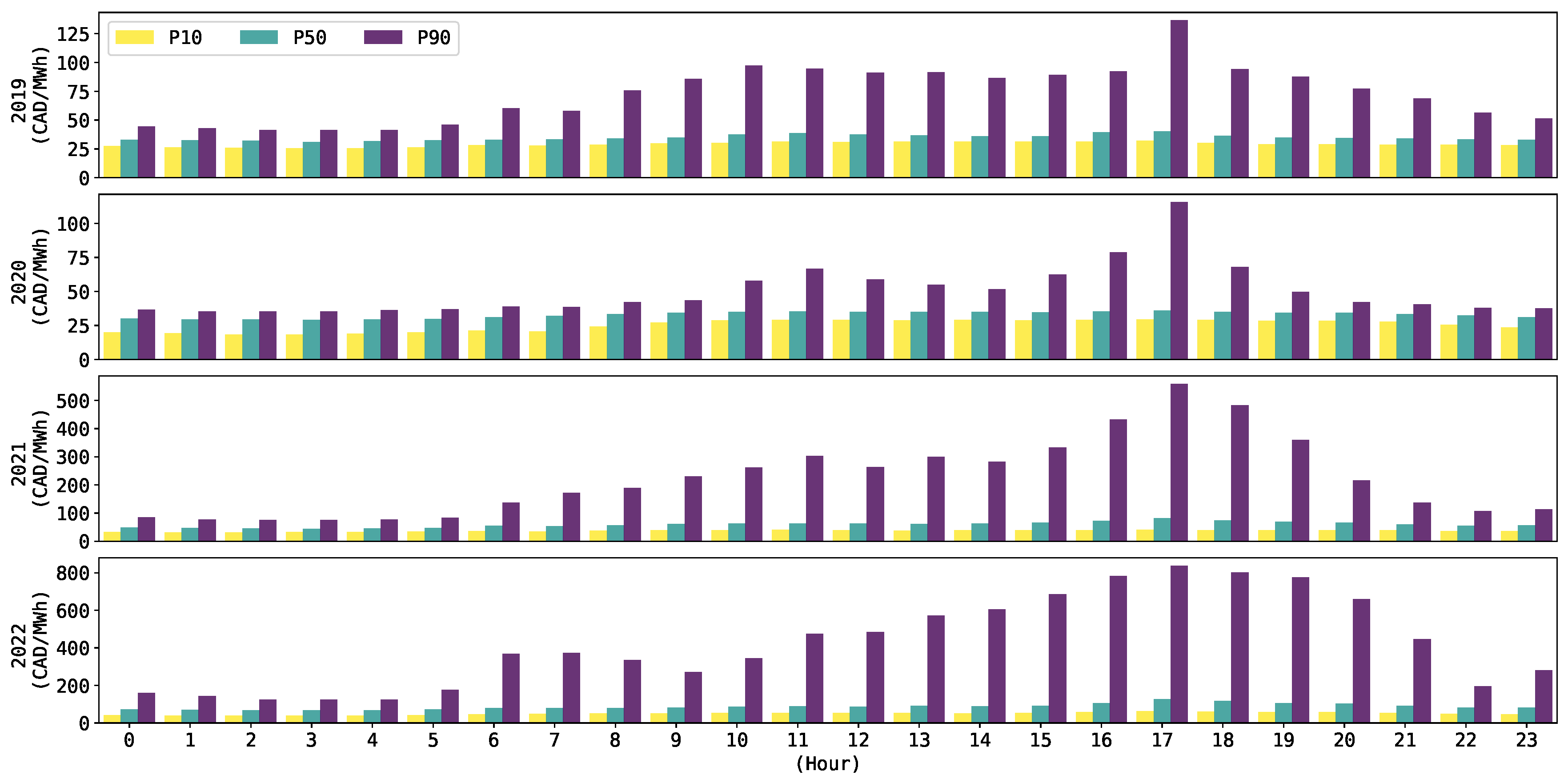
Similarly as made by [8] for the Australian market, Figure 1 shows the 10, 50, and $90\%$ percentiles (i.e., P10, P50, and P90) of the pool price dynamics in Alberta’s market for the years where class predictions ${\widehat{c}}_k$ are generated.

Observe, for example, the tendency of the P10 and P50 for all of the years in Figure 1 to not exceed 100 CAD/MWh at any hour of the day. Conversely, the P90 shows drastic changes when comparing between the years of 2019 and 2020 (e.g., approximately between 125 CAD/MWh and 100 CAD/MWh) against 2021 and 2022 (e.g., approximately between 500 CAD/MWh and 800 CAD/MWh). The diverse high price dynamics, as shown in Figure 1, suggests the convenience of testing the models with different thresholds ${\tau }_{\alpha }^{(·)}$.

The price spike threshold ${\tau }_{\alpha }^{(·)}$ defined in (1) in Section 3, can be represented either as a fixed (${\tau }_{\alpha }^{\left(I\right)}$) or variable (${\tau }_{\alpha }^{\left(II\right)}$) threshold. Let us define the set of fixed thresholds [4,8,21] v in ${\tau }_{\alpha }^{\left(I\right)}$ as the prices above or equal to 100 CAD/MWh, 200 CAD/MWh, 300 CAD/MWh, 400 CAD/MWh, here, expressed as ${\tau }_{100}$, ${\tau }_{200}$, ${\tau }_{300}$, and ${\tau }_{400}$, respectively. Likewise, the set of variable thresholds [3,16] in ${\tau }_{\alpha }^{\left(II\right)}$ is defined by $\mathcal{K}=1$ and $\mathcal{K}=2$, i.e., $\mu +\sigma$ and $\mu +2·\sigma$; and are expressed as ${\tau }_{\mu +\sigma }$, and ${\tau }_{\mu +2·\sigma }$, respectively. For each threshold type, i.e., ${\tau }_{\alpha }^{\left(I\right)}$ and ${\tau }_{\alpha }^{\left(II\right)}$, the corresponding number of spikes is shown in

Table 2. Number of price spikes for thresholds ${\tau }_{\alpha }^{(·)}$ in (1), and each period in our analysis.

	${\mathit{\tau }}_{\mathit{\mu }+\mathit{\sigma }}$	${\mathit{\tau }}_{\mathit{\mu }+2·\mathit{\sigma }}$	${\mathit{\tau }}_{100}$	${\mathit{\tau }}_{200}$	${\mathit{\tau }}_{300}$	${\mathit{\tau }}_{400}$
2019	713	458	442	264	184	144
2020	652	324	306	189	149	136
2021	1060	744	1651	871	615	448
2022	1429	920	3179	1663	1194	939

.

As expected, Table 2 shows that the number of spiky samples decreases as the value of threshold ${\tau }_{\alpha }^{(·)}$ increases for every test period. Observe the notorious increment in the number of spikes in 2021 and 2022, compared to 2019 and 2020. Among others, an important reason for this is due to changes in the bidding strategies of some market participants looking to increase their asset profitability. Thus, resulting in higher market price offers from these market participants [57]. Moreover, observe the number of hourly spiky samples in Table 2 is small compared to, e.g., one year of hourly data. The high imbalance between the spiky and normal prices is one of the reasons why modeling electricity price spikes is a non-trivial task [9].

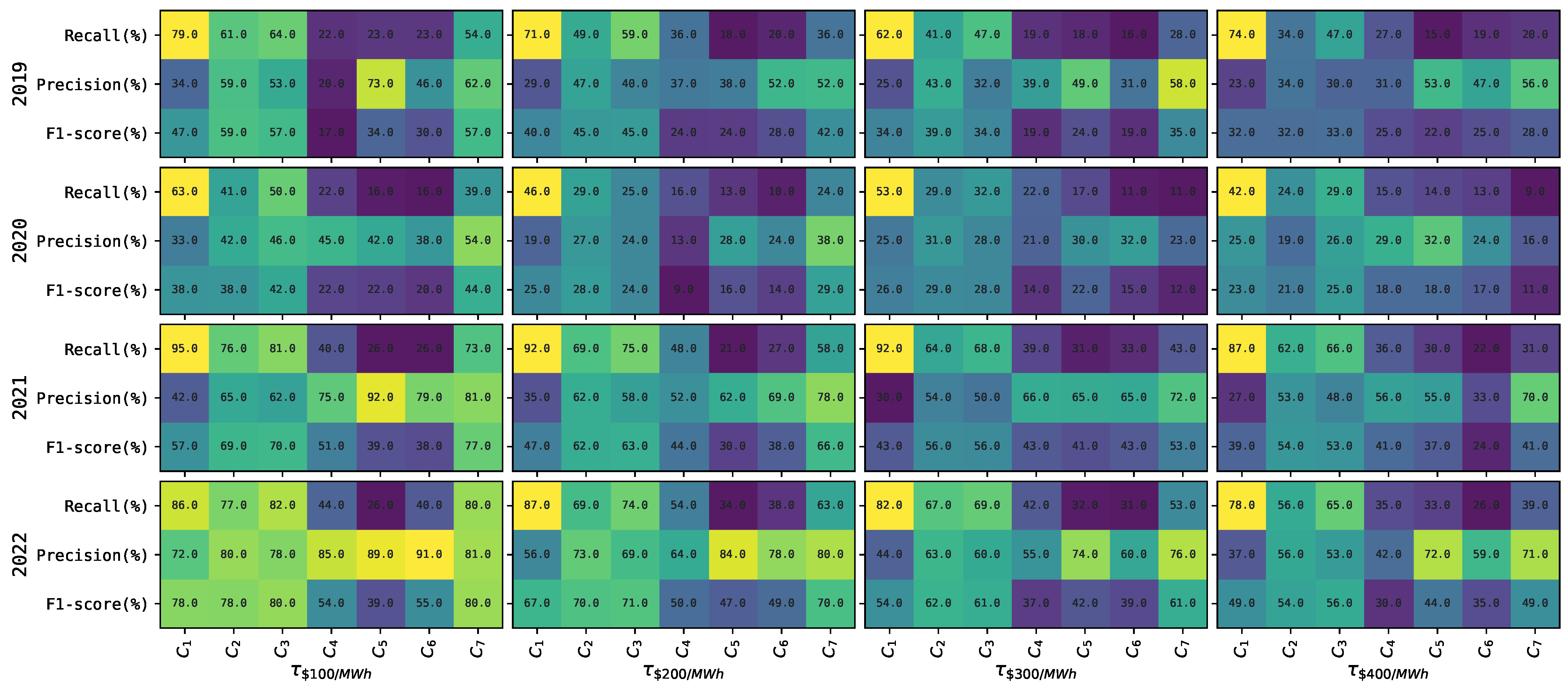
Figure 2 shows the mean recall (2), precision (3) and F1-score (4) for each classifier ${\mathcal{C}}_k$, and threshold ${\tau }_{\alpha }^{\left(I\right)}$ across the tests periods. Here, the value of each threshold in ${\tau }_{\alpha }^{\left(I\right)}$ remains fixed through every training period m. For each of these performance metrics, Figure 2 shows a general tendency for classifiers ${\mathcal{C}}_k$ to decrease their performance as the value of the threshold increases. For example, for most of the years, performance metrics, and threshold ${\tau }_{\alpha }^{\left(I\right)}$, we observe this tendency to occur for more than 75% (and up to 90%) of the time. The only exception is 2020, where this only occurs 63% of the time.

Furthermore, Figure 2 shows that in 2020, classifiers ${\mathcal{C}}_k$ tend to perform lower compared to other years. This is more (less) notorious for classifiers ${\mathcal{C}}_1$ to ${\mathcal{C}}_3$ and ${\mathcal{C}}_7$ (${\mathcal{C}}_4$ to ${\mathcal{C}}_6$). This may probably be associated with the impact of the COVID-19 pandemic on market price dynamics during that year. Furthermore, in general, in all years and thresholds ${\tau }_{\alpha }^{\left(I\right)}$, it is possible to observe that the variations between mean performance metrics are not significant for classifiers ${\mathcal{C}}_2$, ${\mathcal{C}}_3$ and ${\mathcal{C}}_7$. In contrast, these variations in mean performance tend to be significant for classifiers ${\mathcal{C}}_1$ and ${\mathcal{C}}_4$ to ${\mathcal{C}}_6$.

Among all classifiers, ${\mathcal{C}}_1$ tends to show the highest performance to predict the occurrence of price spikes in Figure 2, i.e., see mean recall. However, the lower precision of ${\mathcal{C}}_1$ most times may suggest a possible tendency to overestimate predictions of the occurrence of price spikes. Moreover, in terms of precision, i.e., the capacity of classifier ${\mathcal{C}}_k$ to not overestimate the predictions of the occurrence of price spikes, classifier ${\mathcal{C}}_7$ shows the highest mean precision for most of the cases in Figure 2. Finally, ${\mathcal{C}}_2$ has the highest mean F1-score most of the time but is not as evident as with the recall and precision cases.

Interestingly, Figure 2 shows that classifier ${\mathcal{C}}_4$, optimized with recall, obtains a higher average precision than recall for most of the years and thresholds ${\tau }_{\alpha }^{\left(I\right)}$. A possible reason for this is that the explainable model requires, among others, a minimum recall and precision as hyperparameters to select the best-performing rules (see Appendix A.2). Here, for example, when optimized with ${\mathcal{E}}_j^{*}$ where $\in j=${recall}, we use a search range within a minimum recall (precision) of $[0.3,0.7]$$\left(\right[0.01,0.02\left]\right)$. Observe we try to set higher limits for recall than precision, to try to find an optimal rule able to detect as much FN as possible (see (2) in Section 3.2). However, due to the challenging nature of the imbalance problem, as shown in Table 2, the rules seem to have difficulties in achieving such a task.

To corroborate our previous assumption, we run a new simulation for ${\mathcal{C}}_4$ using ${\tau }_{\alpha }^{\left(I\right)}$, where minimum recall is now set using the default hyperparameter, as found in [31], i.e., equal to 0.01. Conversely, we set minimum precision to a ‘high’ range, i.e., $[0.9,0.95]$, to try to enforce the model to ‘easily’ find a higher recall. However, results from this simulation are similar to those in Figure 2 for ${\mathcal{C}}_4$, where higher average precision tends to prevail in most cases. Thus, there may be evidence that empirically shows that in our problem, the extracted rules used to generate predictions ${\widehat{c}}_4$, tend to be better, on average, at detecting FP than FN.

The mean recall, precision, and F1-score for each classifier ${\mathcal{C}}_k$ using a variable threshold in ${\tau }_{\alpha }^{\left(II\right)}$ are presented in Figure 3. A variable threshold ${\tau }_{\alpha }^{\left(II\right)}$ in (1) is estimated using the spot price observed on the last month of each training period (excluding the validation period) m, i.e., month 11. Here, using the last month would allow the threshold to include the most recent possible market information and its impact on the price dynamics.

Observe from Figure 3 that the performance of the classifiers ${\mathcal{C}}_k$ also tends to decrease as the threshold ${\tau }_{\alpha }^{\left(II\right)}$ increases. In general, this occurs on average 88% of the time for all thresholds, performance metrics, and most test periods.

Figure 3 shows that the classifier with the best mean recall across all thresholds ${\tau }_{\alpha }^{\left(II\right)}$ and test periods is again ${\mathcal{C}}_1$. Moreover, in this case, classifier ${\mathcal{C}}_5$ shows the highest mean precision most of the time for thresholds ${\tau }_{\alpha }^{\left(II\right)}$. Regarding the F1-score, ${\mathcal{C}}_3$ has the highest one for most of the cases when compared to other classifiers. Again, we observe that classifiers ${\mathcal{C}}_1$, and ${\mathcal{C}}_4$ to ${\mathcal{C}}_6$ have a higher variability between mean recall, precision and F1-score. In contrast, ${\mathcal{C}}_2$, ${\mathcal{C}}_3$, and ${\mathcal{C}}_7$ tend to show a more stable mean performance across these metrics.

Again, we observe that the classifier ${\mathcal{C}}_4$ has a higher mean precision than recall. Here, since the hyperparameter search space for minimum recall (precision) is the same regardless of the price spike threshold ${\tau }_{\alpha }^{(·)}$, we believe the same idea, as previously explained for Figure 2, prevails.

General conclusions are derived from Figure 2 and Figure 3. For any threshold type, classifier ${\mathcal{C}}_1$, i.e., optimized to enhance recall performance, heavily trades-off precision and, therefore, F1-score. As previously stated, this may be an indication of this classifier overestimating the class predictions of price spikes. For the generality of this conclusion, we try to investigate if in our experiment, classifier ${\mathcal{C}}_4$ would behave similarly to ${\mathcal{C}}_1$. That is, if instead of using ${\mathcal{C}}_4$’s rules to generate the predictions (i.e., see Algorithm 1 in Section 3.4), we use the model, i.e., as with any machine learning algorithm. We run our experiment for ${\mathcal{C}}_4$ following these ideas. Results are shown in

Table 3. Mean statistical performance $E_i$ for ${\mathcal{C}}_4$ and ${\tau }_{\alpha }^{\left(II\right)}$ when the model, and not the extracted rules are used to generate predictions ${\widehat{c}}_4$.

	Recall (%)		Precision (%)		F1-Score (%)
	${\tau }_{\mu +\sigma }$	${\tau }_{\mu +2·\sigma }$	${\tau }_{\mu +\sigma }$	${\tau }_{\mu +2·\sigma }$	${\tau }_{\mu +\sigma }$	${\tau }_{\mu +2·\sigma }$
2019	80	80	21	7	27	12
2020	69	62	21	12	26	14
2021	88	93	17	17	25	24
2022	87	74	21	16	31	24

.

For the sake of preserving space, Table 3 shows the results of the experiment only for ${\tau }_{\alpha }^{\left(II\right)}$. However, similar results are observed for ${\tau }_{\alpha }^{\left(I\right)}$. Observe that, when predictions ${\widehat{c}}_4$ are generated using ${\mathcal{C}}_4$ as a model, its performance tends to be biased towards increasing the recall at the cost of decreasing precision and F1-score; as observed with ${\mathcal{C}}_1$. Thus, in our experiment, ${\mathcal{C}}_1$’s derived conclusion is extended to ${\mathcal{C}}_4$, only if rules from ${\mathcal{C}}_4$, are not used to generate predictions.

In contrast, for those classifiers optimized to improve precision and F1-score performance, i.e., ${\mathcal{C}}_2$ and ${\mathcal{C}}_3$, and, ${\mathcal{C}}_5$ and ${\mathcal{C}}_6$, the optimal set of hyperparameters appears to be those decreasing the chances of overestimating (higher precision) the occurrence of a price spike, at the cost of underestimating (lower recall) them. This idea applies to classifier ${\mathcal{C}}_7$, too.

It is difficult to observe a general tendency for a classifier ${\mathcal{C}}_k$ to have a significantly better statistical performance for thresholds in ${\tau }_{\alpha }^{\left(I\right)}$ than those in ${\tau }_{\alpha }^{\left(II\right)}$. Finally, in the proposed investigation study, observing a single model achieving high performance across the different error metrics, is challenging. A similar conclusion is derived in [4,8].

4.2. Economic Evaluation of the Occurrence of Price Spike Predictions

Based on the statistical performance of a classifier ${\mathcal{C}}_k$ in Figure 2 and Figure 3, we evaluate the economic implications of the forecasts ${\widehat{c}}_k$ based on the threshold ${\tau }_{\alpha }^{(·)}$ in the decision making of a market participant. This is achieved following (5c) and (6) in Section 3.2. The example case study evaluates a demand-side management strategy [38] for a 1 MW load $\gamma$. In other words, we quantify the economic value of the forecasts using a one-sided approach [42]. Finally, this application can be extended to other markets, too.

For each threshold ${\tau }_{\alpha }^{(·)}$ and test period, we first quantify the total profit or loss for operating $\gamma$ following (6) in Section 3.3. Therefore, for all thresholds in ${\tau }_{\alpha }^{\left(I\right)}$, the total profits $\mathcal{B}$ are CAD 299,165; CAD 3,805,565; CAD 7,311,965, and CAD 10,818,365, respectively. Likewise, for thresholds in ${\tau }_{\alpha }^{\left(II\right)}$, total profits $\mathcal{B}$ correspond to CAD 3,192,417 and CAD 6,675,959 respectively. Using these profits as a base comparison, we evaluate if operating load $\gamma$ based on forecasts from classifier ${\mathcal{C}}_k$, represents an economic benefit.

Table 4. Difference, in thousand CAD, ${\mathsf{\Pi }}_k-\mathcal{B}$ for ${\tau }_{\alpha }^{\left(I\right)}$ corresponding to the total of the test period. The best results are shown in bolted letter.

(Thousand CAD)	${\mathcal{C}}_1$	${\mathcal{C}}_2$	${\mathcal{C}}_3$	${\mathcal{C}}_4$	${\mathcal{C}}_5$	${\mathcal{C}}_6$	${\mathcal{C}}_7$
${\tau }_{100}$	2,210	2,284	2,327	1,460	1,246	1,582	2,328
${\tau }_{200}$	939	1,331	1,333	413	850	978	1,419
${\tau }_{300}$	277	836	797	−10	713	704	914
${\tau }_{400}$	−268	470	388	−98	422	340	593

shows the total profit (positive) or loss (negative) from the difference between ${\mathsf{\Pi }}_k-\mathcal{B}$ for each classifier ${\mathcal{C}}_k$ and fixed threshold ${\tau }_{\alpha }^{\left(I\right)}$. Here, it is shown that load $\gamma$ benefits the most using predictions from classifier ${\mathcal{C}}_7$. As referenced from Section 4.1, Figure 2 shows ${\mathcal{C}}_7$ as the model with the highest mean precision performance for most of the cases. Moreover, as discussed in Section 4.1, ${\mathcal{C}}_7$ benefits from having a more stable mean predictive performance for all metrics, most of the time. From a practical perspective, it means an optimal balance between FP and FN predictions in (2) and (3); thus, translating into less economic damage reflected in ${\mathsf{\Pi }}_7$.

For example, ${\mathcal{C}}_7$ has a lower total economic loss due to the overestimation of predictions of the occurrence of price spikes for ${\tau }_{400}$ but not for ${\tau }_{100},{\tau }_{200}$, and ${\tau }_{300}$, being ${\mathcal{C}}_5$ the one with the lowest economic losses. However, for all thresholds ${\tau }_{\alpha }^{\left(I\right)}$, ${\mathcal{C}}_7$ benefits from having much lower losses than ${\mathcal{C}}_5$ due to the underestimation of predictions of the occurrence of price spikes. The total sum of these losses i.e., underestimation plus overestimation, corresponds to −CAD 631,974 and −CAD 1,644,171 for ${\mathcal{C}}_7$ and ${\mathcal{C}}_5$, respectively.

Likewise, Table 4 shows that ${\mathcal{C}}_1$ has a high economic loss when the threshold is ${\tau }_{400}$. Nevertheless, we also observe that there is a profit for the other thresholds for ${\mathcal{C}}_1$. However, to contrast with the ideas based on observations from Figure 2, our numerical results show that ${\mathcal{C}}_1$ has the highest economic losses due to FP among all classifiers ${\mathcal{C}}_k$ for ${\tau }_{100}$, ${\tau }_{300}$, and ${\tau }_{400}$. These losses represent −CAD 134,032; −CAD 463,566, and −CAD 555,493, respectively. For ${\tau }_{200}$, the highest loss is for ${\mathcal{C}}_4$ (i.e., −CAD 379,676), but just CAD 2,182 higher than ${\mathcal{C}}_1$. In contrast, ${\mathcal{C}}_1$ has the lowest economic losses due to FN (i.e., −CAD 42,190; −CAD 43,450; −CAD 36,212 and −CAD 26,892, respectively) across all thresholds. Thus, as previously mentioned, ${\mathcal{C}}_1$ shows a tendency to trade off high levels of recall with low levels of precision.

In regards to ${\mathcal{C}}_4$, Table 4 shows negative economic impacts in ${\tau }_{300}$ and ${\tau }_{400}$. Figure 2 shows that ${\mathcal{C}}_4$ has a tendency that, on average, benefits precision over recall, however, this is not restrictive for all the periods. For instance, take ${\mathcal{C}}_4$ when ${\tau }_{400}$ in Table 4. Here, our results show that in August 2022, ${\mathcal{C}}_4$ incurs a big economic loss associated with the overestimation of the occurrence of price spikes. Moreover, the recall is high but precision is low in this period. Thus, negatively affecting the total ${\mathsf{\Pi }}_4-\mathcal{B}$.

Table 5. Difference, in thousand Canadian dollars (CAD), ${\mathsf{\Pi }}_k-\mathcal{B}$ for ${\tau }_{\alpha }^{\left(II\right)}$ corresponding to the total of the test period. The best results are shown in bolted letter.

(Thousand CAD)	${\mathcal{C}}_1$	${\mathcal{C}}_2$	${\mathcal{C}}_3$	${\mathcal{C}}_4$	${\mathcal{C}}_5$	${\mathcal{C}}_6$	${\mathcal{C}}_7$
${\tau }_{\mu +\sigma }$	998	1,316	1,325	858	879	1,139	1,392
${\tau }_{\mu +2·\sigma }$	261	810	799	−65	721	325	910

shows the economic results of operating load $\gamma$ using a variable threshold ${\tau }_{\alpha }^{\left(II\right)}$. These results are also obtained as the difference between (5c) and (6) introduced in Section 3, i.e., ${\mathsf{\Pi }}_k-\mathcal{B}$.

It is also possible to observe from Table 5 that the best economic results for both thresholds in ${\tau }_{\alpha }^{\left(II\right)}$, correspond again to classifier ${\mathcal{C}}_7$. From Figure 3, we show ${\mathcal{C}}_5$ as the model with the highest precision most of the time. However, the variability between metrics in terms of average performance is higher when compared to ${\mathcal{C}}_7$. For instance, the economic impact due to FP is less (bigger) for ${\mathcal{C}}_5$ (${\mathcal{C}}_7$). Conversely, losses due to FN are smaller (bigger) for ${\mathcal{C}}_7$ (${\mathcal{C}}_5$). The total of these losses represent −CAD 640,739 and −CAD 289,672 for ${\mathcal{C}}_5$ and ${\mathcal{C}}_7$, respectively.

Evidence from Table 5 shows that, when thresholds are variable, the higher trade-off between recall and precision in Figure 3 does not necessarily translate in the highest economic losses for model ${\mathcal{C}}_1$. However, numerical evidence from our results shows that ${\mathcal{C}}_1$ has the highest (lowest) economic losses due to FP (FN) for each threshold in ${\tau }_{\alpha }^{\left(II\right)}$, i.e., the total in −CAD 761,344 (−CAD 50,193), respectively.

Again, we investigate reasons for ${\mathcal{C}}_4$ having a negative impact, i.e., observe ${\tau }_{\mu +2·\sigma }$. Here, for example, during May 2019 and December 2020, ${\mathcal{C}}_4$ profits ${\mathsf{\Pi }}_4$ are affected by the negative economic impact due to overestimation of the occurrence of price spikes. These balances are observed to significantly trade off good recall against a bad precision score in these months. Thus, negatively impacting the difference ${\mathsf{\Pi }}_4-\mathcal{B}$, and hence the total accounted for ${\tau }_{\mu +2·\sigma }$.

In general, results from Table 4 and Table 5 show that classifiers ${\mathcal{C}}_2$, ${\mathcal{C}}_3$, ${\mathcal{C}}_5$, ${\mathcal{C}}_6$ and ${\mathcal{C}}_7$ consistently generate predictions that economically benefit the operation of load $\gamma$ when compared to the blind operation benchmark $\mathcal{B}$, using threshold ${\tau }_{\alpha }^{(·)}$. Moreover, these results demonstrate that, in price spike occurrence forecasting, a higher performance in one statistical error metric, would not necessarily translate into a high economic benefit [35], e.g., ${\mathcal{C}}_1$ in our study. Likewise, in contrast to [8], who concludes that a false negative of the probability of occurrence of a price spike would be more detrimental for an energy retailer than a false positive, our results suggest that a balance between recall and precision, with some bias towards the latter, brings higher economic benefits for the proposed case study, i.e., see ${\mathcal{C}}_7$. This conclusion extends to ${\mathcal{C}}_2$ and ${\mathcal{C}}_3$, whose results are also competitive. Moreover, based on ${\mathcal{C}}_7$’s performance, our results are better aligned to those in [35]. Here, the authors show the spike prediction confidence (i.e., precision) translates as beneficial in the cost-benefit analysis for the supply bids of a market participant in the Australian market. Finally, we agree with [35], who emphasizes the importance of integrating the price spike forecasting method with the decision-making process.

4.3. The Trade-Off between Performance and Explainability

In recent years, interpretable AI in energy forecasting has started to capture the attention of researchers. The goal is to enhance the acceptability of AI models with the industry stakeholders [5,29]. Additionally, interpretability allows for the comparison between expert knowledge and model decisions. This is particularly important, for example, in the engineering field [43]. However, the methodological trade-offs between a model’s performance and interpretability [43] remain as a challenge. Here, to the best of our knowledge, the economic impact of this trade-off on a market’s participant has not been explored yet in price spike occurrence forecasting.

In this investigative study, we quantify the trade-off between model predictive performance and interpretability. Results in Table 4 and Table 5 show that, for the proposed case study, ${\mathcal{C}}_7$ is the model that brings the highest profits with respect to ${\mathsf{\Pi }}_7-\mathcal{B}$, among all models ${\mathcal{C}}_k$ and thresholds ${\tau }_{\alpha }^{(·)}$. Moreover, among the explainable classifiers ${\mathcal{C}}_4$ to ${\mathcal{C}}_6$, ${\mathcal{C}}_5$ and ${\mathcal{C}}_6$ tend to be competitive across thresholds ${\tau }_{\alpha }^{(·)}$ in ${\mathsf{\Pi }}_5-\mathcal{B}$ and ${\mathsf{\Pi }}_6-\mathcal{B}$. Thus, we arbitrarily pick ${\mathcal{C}}_5$ for showcasing purposes.

Table 6. The total profits and differences, in thousand Canadian dollars (CAD), for the best performing not interpretable model ${\mathcal{C}}_7$ and the interpretable model ${\mathcal{C}}_5$ across all test periods and threshold ${\tau }_{\alpha }^{(·)}$ types.

(Thousand CAD)	${\mathit{\tau }}_{100}$	${\mathit{\tau }}_{200}$	${\mathit{\tau }}_{300}$	${\mathit{\tau }}_{400}$	${\tau }_{\mu +\sigma }$	${\tau }_{\mu +2·\sigma }$
${\mathcal{C}}_5$	1,545	4,655	8,025	11,240	4,072	7,397
${\mathcal{C}}_7$	2,627	5,225	8,226	11,411	4,585	7,586
${\mathcal{C}}_7-{\mathcal{C}}_5$	1083	569	202	171	513	189

shows the economic trade-off between the model’s performance and interpretability for the demand-side management case in this study. For the sake of showing the idea behind this trade-off in price spike forecasting, we are comparing the best non-interpretable performing model, i.e., ${\mathcal{C}}_7$, against a competitive interpretable model, i.e., ${\mathcal{C}}_5$.

For the demand-side management application, the economic differences between ${\mathcal{C}}_7$ and ${\mathcal{C}}_5$ displayed in Table 6 for each spike threshold ${\tau }_{\alpha }^{(·)}$, represent the trade-off due to the lost of ${\mathcal{C}}_5$’s statistical forecasting performance. These differences indicate that, if one would pick using human-interpretable decision rules from ${\mathcal{C}}_5$ to predict the occurrence of price spikes at any selected threshold ${\tau }_{\alpha }^{(·)}$, the cost of it would have been ${\mathcal{C}}_7-{\mathcal{C}}_5$ for each case, respectively. Finally, observe from Table 4 and Table 5 that forecasts from ${\mathcal{C}}_5$ would still have economically benefited the operation of load $\gamma$.

Predictions ${\widehat{c}}_5$ are made using decision rules from the explainable model introduced in Appendix A.2. Here, we show an example of a decision rule used to generate forecasts ${\widehat{c}}_5$ during July 2022 using ${\tau }_{200}$ [21]. We select this period because it corresponds to the Summer season, where price spikes are likely to occur due to the high demand associated with extreme temperatures [8,57].

Thus, the decision rule used to generate the class price spike forecasts is pool_price_lag_1 > 379 AND wind_7d_forecast_lag_24 > 26. This predictive rule has a recall, precision, and F1-score of 53.6, 87, and 66.3%, respectively. Observe that this rule has a cardinality of two, and is the best-performing rule selected from the semantic deduplication process introduced in Appendix A.2. In other words, two features from the total in $\mathbf{X}\in \mathbb{R}$ (i.e., see Section 3) have been found by Skope Rules [31] as relevant, to generate one-hour-ahead forecasts of the occurrence of price spikes during July 2022 using threshold ${\tau }_{200}$.

5. Conclusions

An investigation study involving the statistical and economic performance analysis of the forecasts of the occurrence of electricity price spikes was proposed in this paper. Here, a set of different fixed and variable electricity spike thresholds were used. Moreover, interpretable and non-interpretable classification- and regression-based price spike models were trained using data from Alberta’s power market. We investigated the impact that using various statistical error metrics on the hyperparameter optimization process of the models, had on predicting the occurrence of these spikes. The final forecasts were evaluated using the same set of statistical metrics, and also by quantifying their economic impact using a demand-side management strategy. We compared against a simple economic benchmark. Finally, we quantified the so-called trade-off between the model’s performance and interpretability using an interpretable and a non-interpretable model.

Simulation results showed that hyperparameter optimization with recall tends to control underestimation but not overestimation of the occurrence of price spikes. Conversely, if precision or F1-score are used, this trade-off tends to be better balanced. This tendency was observed, in general, regardless of the price spike threshold. The economic results from the demand-side management case study further confirmed this balance as optimal. In general, these results reflected that is better to avoid an excessive overestimation of the spiky predictions, without heavily sacrificing their underestimation. Finally, in the proposed investigative methodology, interpretability has a high cost for the example study case. In general, we argue that interpretability adds additional difficulties to the already challenging task of predicting price spikes. However, we recognize that interpretability is an active field of research, and the exploration and integration of more robust interpretable methods could be a future research path in electricity price spike forecasting.

One limitation of this research work is that we did not conduct experiments using different cut-off probabilities for the classification-based models. Thus, we let this as future work, along with experimenting with different ensembles of models, which have proven to be competitive in electricity price forecasting. Finally, the statistical evaluation metrics in this study follow those commonly used by some other works in price spike forecasting, however, we recognize that alternative metrics can be worth investigating for this task. Therefore, we leave this as a path for future research.

References

- Weron, R. Electricity price forecasting: A review of the state-of-the-art with a look into the future. Int. J. Forecast. 2014, 30, 1030–1081. [Google Scholar] [CrossRef]
- Zhang, C.; Fu, Y.; Gong, L. Electricity Price Forecast Using Frequency Analysis and Price Spikes Oversampling. IEEE Trans. Power Syst. 2023, 38, 4739–4751. [Google Scholar] [CrossRef]
- Zhao, J.H.; Dong, Z.Y.; Li, X.; Wong, K.P. A Framework for Electricity Price Spike Analysis with Advanced Data Mining Methods. IEEE Trans. Power Syst. 2007, 22, 376–385. [Google Scholar] [CrossRef]
- Eichler, M.; Grothe, O.; Manner, H.; Tuerk, D. Models for Short-Term Forecasting of Spike Occurrences in Australian Electricity Markets: A Comparative Study. J. Energy Mark. 2014, 7, 55–81. Available online: https://ssrn.com/abstract=2789605 (accessed on 9 December 2023). [CrossRef]
- Bottieau, J.; Wang, Y.; De Greve, Z.; Vallee, F.; Toubeau, J. Interpretable Transformer Model for Capturing Regime Switching Effects of Real-Time Electricity Prices. IEEE Trans. Power Syst. 2023, 38, 2162–2176. [Google Scholar] [CrossRef]
- Hong, T.; Pinson, P.; Fan, S.; Zareipour, H.; Troccoli, A.; Hyndman, R. Probabilistic Energy Forecasting: Global Energy Forecasting Competition 2014 and Beyond. Int. J. Forecast. 2016, 32, 896–913. [Google Scholar] [CrossRef]
- Zareipour, H.; Bhattacharya, K.; Cañizares, C. Electricity Market Price Volatility: The Case of Ontario. Energy Policy 2007, 35, 4739–4748. [Google Scholar] [CrossRef]
- Christensen, T.; Hurn, A.; Lindsay, K. Forecasting spikes in electricity prices. Int. J. Forecast. 2012, 28, 400–411. [Google Scholar] [CrossRef]
- Maryniak, P.; Weron, R. What is the Probability of an Electricity Price Spike? Evidence from the UK Power Market. In Handbook of Energy Finance: Theories, Practices and Simulations; Goutte, S., Nguyen, D., Eds.; World Scientific: Hackensack, NJ, USA, 2019; pp. 231–245. [Google Scholar]
- Mayer, K.; Trück, S. Electricity Markets Around the World. J. Commod. Mark. 2018, 9, 77–100. [Google Scholar] [CrossRef]
- Lago, J.; De Ridder, F.; De Schutter, B. Forecasting Spot Electricity Prices: Deep Learning Approaches and Empirical Comparison of Traditional Algorithms. Appl. Energy 2018, 221, 386–405. [Google Scholar] [CrossRef]
- Sgarlato, R.; Ziel, F. The Role of Weather Predictions in Electricity Price Forecasting Beyond the Day-Ahead Horizon. IEEE Trans. Power Syst. 2023, 38, 2500–2511. [Google Scholar] [CrossRef]
- Lu, Y.; Suthaharan, N. Electricity price spike clustering: A zero-inflated GARX approach. Energy Econ. 2023, 124, 106834. [Google Scholar] [CrossRef]
- Manner, H.; Türk, D.; Eichler, M. Modeling and Forecasting Multivariate Electricity Price Spikes. Energy Econ. 2016, 60, 255–265. [Google Scholar] [CrossRef]
- Lu, X.; Dong, Z.Y.; Li, X. Electricity market price spike forecast with data mining techniques. Electr. Power Syst. Res. 2005, 73, 19–29. [Google Scholar] [CrossRef]
- Zhao, J.; Dong, Z.; Li, X.; Wong, K. A General Method for Electricity Market Price Spike Analysis. IEEE Power Eng. Soc. Gen. Meet. 2005, 1, 286–293. [Google Scholar] [CrossRef]
- Amjady, N.; Keynia, F. A New Prediction Strategy for Price Spike Forecasting of Day-Ahead Electricity Markets. Appl. Soft Comput. 2011, 11, 4246–4256. [Google Scholar] [CrossRef]
- Sandhu, H.; Fang, L.; Guan, L. Forecasting day-ahead price spikes for the Ontario electricity market. Electr. Power Syst. Res. 2016, 141, 450–459. [Google Scholar] [CrossRef]
- Chitsaz, H.; Zamani-Dehkordi, P.; Zareipour, H.; Parikh, P.P. Electricity Price Forecasting for Operational Scheduling of Behind-the-Meter Storage Systems. IEEE Trans. Smart Grid. 2018, 9, 6612–6622. [Google Scholar] [CrossRef]
- Voronin, S.; Partanen, J. Price Forecasting in the Day-Ahead Energy Market by an Iterative Method with Separate Normal Price and Price Spike Frameworks. Energies 2013, 6, 5897–5920. [Google Scholar] [CrossRef]
- Amjady, N.; Keynia, F. Electricity Market Price Spike Analysis by a Hybrid Data Model and Feature Selection Technique. Electr. Power Syst. Res. 2010, 80, 318–327. [Google Scholar] [CrossRef]
- Vu, D.H.; Muttaqi, K.M.; Agalgaonkar, A.P.; Bouzerdoum, A. A Multi-Feature Based Approach Incorporating Variable Thresholds for Detecting Price Spikes in the National Electricity Market of Australia. IEEE Access. 2021, 9, 13960–13969. [Google Scholar] [CrossRef]
- Manfre Jaimes, D.; Zamudio López, M.; Zareipour, H.; Quashie, M. A Hybrid Model for Multi-Day-Ahead Electricity Price Forecasting considering Price Spikes. Forecasting 2023, 5, 499–521. [Google Scholar] [CrossRef]
- Liu, L.; Bai, F.; Su, C.; Ma, C.; Yan, R.; Li, H.; Sun, Q.; Wennersten, R. Forecasting the occurrence of extreme electricity prices using a multivariate logistic regression model. Energy 2022, 247, 123417. [Google Scholar] [CrossRef]
- Christensen, T.; Hurn, S.; Lindsay, K. It Never Rains but It Pours: Modeling the Persistence of Spikes in Electricity Prices. Energy J. 2009, 30, 25–48. [Google Scholar] [CrossRef]
- Boogert, A.; Dupont, D. When Supply Meets Demand: The Case of Hourly Spot Electricity Prices. IEEE Trans. Power Syst. 2008, 23, 389–398. [Google Scholar] [CrossRef]
- Rudin, C. Stop Explaining Black Box Machine Learning Models for High Stakes Decisions and Use Interpretable Models Instead. arXiv 2019, arXiv:1811.10154. [Google Scholar] [CrossRef]
- Olivares, K.; Challu, C.; Marcjasz, G.; Weron, R.; Dubrawski, A. Neural Basis Expansion Analysis with Exogenous Variables: Forecasting Electricity Prices with NBEATSx. Int. J. Forecast. 2023, 39, 884–900. [Google Scholar] [CrossRef]
- Toubeau, J.; Bottieau, J.; Wang, Y.; Vallee, F. Interpretable Probabilistic Forecasting of Imbalances in Renewable-Dominated Electricity Systems. IEEE Trans. On Sustain. Energy. 2022, 13, 1267–1277. [Google Scholar] [CrossRef]
- Lago, J.; Marcjasz, G.; De Schutter, B.; Weron, R. Forecasting day-ahead electricity prices: A review of state-of-the-art algorithms, best practices and an open-access benchmark. Appl. Energy 2021, 293, 116983. [Google Scholar] [CrossRef]
- Goix, N.; Birodkar, V.; Gardin, F.; Schertzer, J.; Jeong, H.; Kumar, M.; Gramfort, A.; Staley, T.; Tour, T.; Deng, B.C.; et al. scikit-learn-contrib/skope-rules v1.0.1. Zenodo 2020. [Google Scholar] [CrossRef]
- Afanasyev, D.O.; Fedorova, E.A. On the Impact of Outlier Filtering on the Electricity Price Forecasting Accuracy. Appl. Energy 2019, 236, 196–210. [Google Scholar] [CrossRef]
- Zareipour, H.; Janjani, A.; Leung, H.; Motamedi, A.; Schellenberg, A. Classification of Future Electricity Market Prices. IEEE Trans. Power Syst. 2011, 26, 165–173. [Google Scholar] [CrossRef]
- Adline, B.; Ikeda, K. A Hawkes Model Approach to Modeling Price Spikes in the Japanese Electricity Market. Energies 2023, 16, 1570. [Google Scholar] [CrossRef]
- Zhao, J.; Dong, Z.; Li, X. Electricity Market Price Spike Forecasting and Decision Making. IET Gener. Transm. Distrib. 2007, 1, 647–654. [Google Scholar] [CrossRef]
- Nitka, W.; Weron, R. Combining Predictive Distributions of Electricity Prices. Does Minimizing the CRPS Lead to Optimal Decisions in Day-Ahead Bidding? arXiv 2023, arXiv:2308.15443. [Google Scholar] [CrossRef]
- Clements, A.; Herrera, R.; Hurn, A. Modelling interregional links in electricity price spikes. Energy Econ. 2015, 51, 383–393. [Google Scholar] [CrossRef]
- Huang, D.; Zareipour, H.; Rosehart, W.; Amjady, N. Data Mining for Electricity Price Classification and the Application to Demand-Side Management. IEEE Trans. Smart Grid. 2012, 3, 808–817. [Google Scholar] [CrossRef]
- Demir, S.; Kok, K.; Paterakis, N. Statistical Arbitrage Trading across Electricity Markets Using Advantage Actor–Critic Methods. Sustain. Energy Grids Netw. 2023, 34, 101023. [Google Scholar] [CrossRef]
- Janczura, J.; Wójcik, E. Dynamic short-term risk management strategies for the choice of electricity market based on probabilistic forecasts of profit and risk measures. The German and the Polish market case study. Energy Econ. 2022, 110, 106015. [Google Scholar] [CrossRef]
- Marcjasz, G.; Narajewski, M.; Weron, R.; Ziel, F. Distributional neural networks for electricity price forecasting. Energy Econ. 2023, 125, 106843. [Google Scholar] [CrossRef]
- Uniejewski, B. Electricity price forecasting with Smoothing Quantile Regression Averaging: Quantifying economic benefits of probabilistic forecasts. arXiv 2023, arXiv:2302.00411. [Google Scholar]
- Hamilton, R.; Papadopoulos, P. Using SHAP Values and Machine Learning to Understand Trends in the Transient Stability Limit. IEEE Trans. Power Syst. 2023, 39, 1384–1397. [Google Scholar] [CrossRef]
- Rodriguez, C.; Anders, G. Energy Price Forecasting in the Ontario Competitive Power System Market. IEEE Trans. Power Syst. 2004, 19, 366–374. [Google Scholar] [CrossRef]
- Conejo, A.; Contreras, J.; Espínola, R.; Plazas, M. Forecasting Electricity Prices for a Day-Ahead Pool-Based Electric Energy Market. Int. J. Forecast. 2005, 21, 435–462. [Google Scholar] [CrossRef]
- Herrera, R.; González, N. The Modeling and Forecasting of Extreme Events in Electricity Spot Markets. Int. J. Forecast. 2014, 30, 477–490. [Google Scholar] [CrossRef]
- Sarajpoor, N.; Rakai, L.; Arteaga, J.; Amjady, N.; Zareipour, H. Time Aggregation in Presence of Multiple Variable Energy Resources. IEEE Trans. Power Syst. 2023, 39, 587–601. [Google Scholar] [CrossRef]
- Pedregosa, F.; Varoquaux, G.; Gramfort, A.; Michel, V.; Thirion, B.; Grisel, O.; Blondel, M.; Prettenhofer, P.; Weiss, R.; Dubourg, V.; et al. Scikit-learn: Machine Learning in Python. J. Mach. Learn. Res. 2011, 12, 2825–2830. [Google Scholar]
- Shi, W.; Wang, Y.; Chen, Y.; Ma, J. An Effective Two-Stage Electricity Price Forecasting Scheme. Electr. Power Syst. Res. 2021, 199, 107416. [Google Scholar] [CrossRef]
- Chen, T.; Guestrin, C. XGBoost: A Scalable Tree Boosting System. In Proceedings of the 22nd ACM SIGKDD International Conference on Knowledge Discovery and Data Mining, San Francisco, CA, USA, 13–17 August 2016; pp. 785–794. [Google Scholar] [CrossRef]
- Januschowski, T.; Wang, Y.; Torkkola, K.; Erkkilä, T.; Hasson, H.; Gasthaus, J. Forecasting with Trees. Int. J. Forecast. 2021, 38, 1473–1481. [Google Scholar] [CrossRef]
- Breiman, L. Bagging Predictors. Mach. Learn. 1996, 24, 123–140. [Google Scholar] [CrossRef]
- Akiba, T.; Sano, S.; Yanase, T.; Ohta, T.; Koyama, M. Optuna: A Next-generation Hyperparameter Optimization Framework. In Proceedings of the 25th ACM SIGKDD International Conference On Knowledge Discovery and Data Mining, Anchorage, AK, USA, 4–8 August 2019; pp. 2623–2631. [Google Scholar] [CrossRef]
- AESO. Adequacy of Supply. Available online: https://www.aeso.ca/rules-standards-and-tariff/iso-rules/section-202-6-adequacy-of-supply/ (accessed on 5 April 2023).
- Zareipour, H.; Canizares, C.; Bhattacharya, K.; Thomson, J. Application of Public-Domain Market Information to Forecast Ontario’s Wholesale Electricity Prices. IEEE Trans. Power Syst. 2006, 21, 1707–1717. [Google Scholar] [CrossRef]
- Contreras, J.; Espinola, R.; Nogales, F.; Conejo, A.J. ARIMA models to predict next-day electricity prices. IEEE Trans. Power Syst. 2003, 18, 1014–1020. [Google Scholar] [CrossRef]
- AESO. 2021 and 2022 Annual Market Statistics. Available online: https://www.aeso.ca/market/market-and-system-reporting/annual-market-statistic-reports/ (accessed on 3 August 2023).
- Friedman, J. Stochastic gradient boosting. Comput. Statistics Data Anal. 2002, 38, 367–378. [Google Scholar] [CrossRef]
- Interpretability with Diversified-by-Design Rules, Skope Rules, a Python Package. Available online: http://2018.ds3-datascience-polytechnique.fr/wp-content/uploads/2018/06/DS3-309.pdf (accessed on 22 May 2023).
- Friedman, J.; Popescu, B. Predictive Learning via Rule Ensembles. Ann. Appl. Stat. 2008, 2, 916–954. [Google Scholar] [CrossRef]
- Molnar, C. Interpretable Models. In Interpretable Machine Learning: A Guide for Making Black Box Models Explainable, 2nd ed.; Molnar, C.A., Ed.; 2022; Available online: https://christophm.github.io/interpretable-ml-book (accessed on 19 September 2023).
- Breiman, L. Random Forests. Mach. Learn. 2001, 45, 5–32. [Google Scholar] [CrossRef]
- Uniejewski, B.; Nowotarski, J.; Weron, R. Automated Variable Selection and Shrinkage for Day-Ahead Electricity Price Forecasting. Energies 2016, 9, 621. [Google Scholar] [CrossRef]
- Tibshirani, R. Regression Shrinkage and Selection Via the Lasso. J. R. Stat. Soc. Ser. B 1996, 58, 267–288. [Google Scholar] [CrossRef]
Figure 1.
The P10, P50, and P90 for the 24 h spot prices in Alberta’s market.
Figure 2.
Each grid corresponds to a heatmap displaying a color representation of the mean performance of each model in the proposed comparative study. The outer (inner) y-axis displays the four test periods (three evaluation metrics ) introduced in Section 3. Likewise, the outer (inner) part of the x-axis displays the four fixed price spike thresholds (seven classifiers ) introduced in Section 3 (Table 1).
Figure 3.
Each grid corresponds to a heatmap displaying a color representation of the mean performance of each model in the proposed comparative study. The outer (inner) y-axis displays the 4 test periods (3 evaluation metrics ) introduced in Section 3. Likewise, the outer (inner) part of the x-axis displays the two variable price spike thresholds (7 classifiers ) introduced in Section 3 (Table 1).