
Predictive Maintenance Framework for Fault Detection in Remote Terminal Units


1
Department of Energy Systems, University of Thessaly, Gaiopolis Campus, 41500 Larissa, Greece
2
Public Power Corporation, Chalkokondili 22, 10432 Athens, Greece
*
Author to whom correspondence should be addressed.
Forecasting 2024, 6(2), 239-265; https://doi.org/10.3390/forecast6020014
Submission received: 31 December 2023
/
Revised: 16 March 2024
/
Accepted: 21 March 2024
/
Published: 25 March 2024
Abstract
:The scheduled maintenance of industrial equipment is usually performed with a low frequency, as it usually leads to unpredicted downtime in business operations. Nevertheless, this confers a risk of failure in individual modules of the equipment, which may diminish its performance or even lead to its breakdown, rendering it non-operational. Lately, predictive maintenance methods have been considered for industrial systems, such as power generation stations, as a proactive measure for preventing failures. Such methods use data gathered from industrial equipment and Machine Learning (ML) algorithms to identify data patterns that indicate anomalies and may lead to potential failures. However, industrial equipment exhibits specific behavior and interactions that originate from its configuration from the manufacturer and the system that is installed, which constitutes a great challenge for the effectiveness of ML model maintenance and failure predictions. In this article, we propose a novel method for tackling this challenge based on the development of a digital twin for industrial equipment known as a Remote Terminal Unit (RTU). RTUs are used in electrical systems to provide the remote monitoring and control of critical equipment, such as power generators. The method is applied in an RTU that is connected to a real power generator within a Public Power Corporation (PPC) facility, where operational anomalies are forecasted based on measurements of its processing power, operating temperature, voltage, and storage memory.
1. Introduction
Industrial systems are currently undergoing a transformation toward an interconnected area referred to as Industry 4.0 [1]. This transformation is supported by intelligent devices (e.g., sensors, actuators) that communicate seamlessly and in an autonomous manner through the use of Internet of Things (IoT) and Industrial IoT technologies [2].
To maintain autonomous operation and avoid the need for manual human intervention in case of potential failures, the regular maintenance of industrial equipment is required. Determining the maintenance frequency is a challenge and is mainly based on the system where the equipment is deployed, given that a failure in one piece of equipment may also cascade and result in additional ones [3], leading to catastrophic damages in entire industrial systems, such as power plants, with financial, regulatory, and reputational impacts. Moreover, maintenance also aims at improving the operational accuracy, as well as protecting the operators who use the equipment [4].
To tackle this challenge, industries are rapidly adopting predictive maintenance (PdM) solutions [5,6]. PdM is a proactive maintenance technique that utilizes asset data (real-time and historical) in order to determine whether the asset will fail in the future. This is performed by (1) gathering all the relevant data and predicting their future values and (2) performing anomaly detection on the predicted values to intercept potential incidents before they actually happen. Such a provision allows mitigation measures to be initiated to restore the equipment to its full operational status.
However, developing an effective PdM system is challenging, particularly when dealing with production-oriented industrial components. PdM systems entail predicting the Remaining Useful Life (RUL) or detecting anomalies in a component’s future behavior. Based on the existing literature [7], there are currently more than 14 different definitions of anomalies, 39 anomaly detection techniques, and 20 different mitigation techniques for detected anomalies. Despite the importance of dealing with these anomalies adequately, concrete practical guidelines for managing them are scarce, as there is a large variety of approaches and estimation goals tackling the PdM task, which makes it harder to compare results and come to definite conclusions. Moreover, acquiring real run-to-failure data is often difficult, as the long-term tracking of equipment from the initial to the current state is impractical in some cases, and most equipment with sensors is either well designed or routinely fixed before failing.
The existing PdM approach involves predicting the RUL of a machine using operational sensor data by assuming how the system degrades or how a fault evolves. However, this approach may not be suitable for domains where degradation does not follow a pattern, and accurate physical or system models may not be available. Hence, the development of a PdM framework that allows the automation of operational fault detection, as well as the prediction of performance issues or asset deterioration, is deemed necessary for industrial organizations. Nevertheless, the computational burden and the complexity of Deep Learning (DL) models in the literature [8], as well as the overall amount of required data [9], make existing approaches quite challenging and hinder their adoption by non-experts in the field.
To address these challenges, this article proposes a concrete PdM framework of an industrial component, i.e., a Remote Terminal Unit (RTU), in order to monitor and track its health status. The proposed PdM is data-driven and uses different ML and statistical models. Specifically, time-series forecasting models are used to predict the RTU’s state as far into the future as possible, and unsupervised anomaly detection models are employed to detect possible anomalies in the forecasted data, even in the absence of failure data. In particular, this article makes the following contributions:
- The design flow of a PdM framework for the detection of potential anomalies leading to failures in industrial infrastructure equipment, such as RTUs.
- The implementation and comparison of time-series ML models for forecasting the RTU operational status using features such as processing power, memory, operating temperature, and voltage.
- The detection of anomalies in the operational status of the RTU based on various ML models, which are also compared in terms of performance and anomaly prediction accuracy.
- The real-life application of the proposed PdM framework and integration with a power generator in the industrial infrastructure of a PPC.
The rest of this article is organized as follows. Section 2 presents background information on the electrical infrastructure equipment, specifically focusing on RTU functionalities as well as a brief overview of the PdM and anomaly detection modules toward building a DT. Then, Section 3 describes the PdM framework based on individual time-series forecasting and anomaly detection modules. The PdM framework is then validated in Section 4 through a case study using an RTU that is deployed in the industrial infrastructure of a PPC. Section 5 provides the benefits and limitations of the proposed method, as well as related work and challenges towards the positioning of the work alongside the current state of the art. Finally, Section 6 provides conclusions and some perspectives for future work.
2. Preliminaries
In this section, we provide an overview of the industrial equipment, i.e., RTUs, to which our method is applied, as well as a description of the PdM and its significance in the process of building a DT.
2.1. Remote Terminal Units
RTUs are used to remotely monitor and control a variety of electronic equipment in order to ensure their real-time operational availability. RTUs typically have a network of embedded devices (e.g., sensors, actuators) to facilitate their connection to the equipment they are monitoring or controlling. These devices allow them to gather data and analyze them to facilitate decisions on how the electronic equipment will be operated. Often, when additional processing resources are needed, the data are also sent to central control stations for further analysis. This is especially useful in situations where the electronic equipment is located in remote or hard-to-reach locations, such as distant electrical grid substations, where it is not practical or cost-effective to have a human operator present at all times.
Figure 1 illustrates an RTU deployed in PPC industrial infrastructure and connected near a power generator. The generator produces energy from diesel fuel and distributes it to residential areas. The RTU gathers operational data from the power generator, which can be later analyzed to deduce performance metrics. The causes of an RTU’s physical degradation may include thermal and electrical stress, mechanical wear, environmental corrosion, or firmware/software obsolescence. The operational and environmental stress factors contributing to each failure mechanism may include temperature variations, voltage fluctuations, physical vibration levels, humidity, or dust exposure, which depend on the RTU manufacturer characteristics as well as the deployed environment.
As a consequence, degradation may decrease the RTU performance such that it will be unable to analyze the operational data. In turn, this may lead to a reduction in produced energy; hence, it is usually necessary that this be predicted before it actually happens. When predictions are accurate, the RTU or the equipment it controls, such as a power generator, is promptly scheduled for maintenance, which prevents any degradation in the performance, as well as any reduction in the amount of produced energy.
When connected to such critical equipment as a power generator, the RTU collects data such as the operating temperature, voltage, memory, and processing power (i.e., CPU). It is crucial to continuously monitor these parameters to ensure the safe and efficient operation of the power generator and other industrial equipment controlled by the RTU, as anomalies in the data collected by the RTU could lead to information loss and not indicate potential issues with the power generator, which could go undetected. For example, a sudden increase in the temperature and CPU usage of the RTU could lead to unexpected behaviors such as delays, or the RTU could be overloaded and shut down automatically. Unplanned downtime of the RTU prevents it from monitoring the health status of the power generator and other equipment and can have a significant impact on the production of energy and result in significant financial losses. This work focuses on tackling this challenge through the use of a PdM framework to ensure the early-stage detection of potential failures in the RTU, as well as in the equipment it controls. Thus, a brief description of PdM and how it is employed as one of the core modules of a Digital Twin (DT) is provided in the following section.
2.2. Predictive Maintenance as a Digital Twin Module
DTs are digital representations of physical processes or real systems. They are formed by gathering data from the real system and applying them to reconstruct its behavior and provide feedback to the physical process about possible future outcomes, such as predictions of errors and faults or component maintenance. DT feedback improves the efficiency of the physical process as well as decision-making. Specifically, a DT framework’s goal lies in estimating, forecasting, or monitoring a component’s, system’s, or system-of-system’s state, with an emphasis on estimating the physical system’s response to an unexpected event before it occurs [10].
DTs usually comprise (1) the physical process, (2) a digital model of that physical process (e.g., a statistical or an ML model), (3) data analytics techniques, (4) communication mechanisms between the physical process and the digital model [11]. Many different techniques have been applied to develop DTs, depending on the available data and the desired output. The predicted output of a DT can be divided into classification and regression tasks. Categorical objectives, like machine states, are indicated by a classification task. Continuous objectives, such as the Remaining Useful Life (RUL) before a machine breaks, are indicated by regression tasks.
A module that is usually among the core elements making up a DT is PdM. The reason is that PdM is used for real-time predictions of potential equipment errors/faults or possible maintenance. PdM may also focus on locating potential improvement areas for the physical processes or its individual components, which can be used to maximize performance. Overall, four different types of maintenance mechanisms are present, which are described below:
- Reactive maintenance: A problem that has already happened is fixed to sustain the system’s nominal operational status.
- Preventative maintenance: Routine maintenance tasks are performed periodically to prevent failures. However, often, preventative maintenance is performed despite not actually being necessary, wasting useful resources.
- Rule-based PdM: Maintenance is carried out on the basis of hard-coded threshold rules, and an alert is sent if a measurement crosses the predefined thresholds.
- Machine learning (ML)-based PdM: Advanced analytics and DT techniques are used to forecast when the next failure will occur, and, in response, early-stage maintenance is scheduled.
The most prominent maintenance type is ML-based PdM, which allows the scheduling of maintenance for components of a physical process before it starts malfunctioning. This decreases downtime and increases productivity, as repair is scheduled upon observing potential issues and before the equipment experiences severe faults. Specifically, ML-based PdM usually consists of two sequential parts. Initially, time-series forecasting ML models are applied, which allow for forecasting the behavior of the system. Then, health indication techniques, such as anomaly detection ML models, are applied to the previously forecasted data in order to detect anomalies or predict the RUL of the component.
2.2.1. Time-Series Forecasting Models
To allow the forecasting of time-series values of industrial equipment, different types of models can be applied. First, Long Short-Term Memory (LSTM) [12] is an extension of Recurrent Neural Networks (RNNs), which use previous information for future tasks. However, RNNs suffer from the vanishing and exploding gradient problems, which restrain their memory capabilities. Extending from RNNs, LSTMs provide the capability of “long-term memory” by introducing a mechanism called the “memory cell”, which can maintain information for longer periods of time. An LSTM network is composed of a series of LSTM cells, each of which contains several gates that control the flow of information into and out of the cell. The gates are used to decide what information should be passed to the cell, what information should be discarded, and what information should be passed to the output.
Another well-known forecasting model is the Autoregressive Integrated Moving Average (ARIMA) [13]. ARIMA includes differencing to handle non-stationarity in time-series data and is a linear model that combines the qualities of both moving average (MA) and autoregressive (AR) models. ARIMA can also be combined with grid search, which is a technique used to find the optimal set of hyperparameters for a model by exhaustively searching through a predefined grid of parameter combinations. The AR and MA models are defined by Equations (1) and (2), respectively. The ARIMA model is characterized by three parameters: p, d, and q. The number of lag observations used to predict the current value is indicated by the parameter p, which stands for the order of the autoregressive equipment. The number of lag errors used to forecast the current value is represented by the parameter q, which stands for the order of the moving average component. Finally, indicates white noise. The equation of a typical autoregressive model is
Likewise, the equation of a typical moving average model is
Equation (1) also shows that the future value is computed as a weighted linear combination of errors made by the model at previous time steps. The value q denotes the window defining how far into the past we are willing to look to decide the value of . So, the above model is a moving average model of order q, or simply . When performing grid search for ARIMA, the hyperparameters to consider are typically denoted by p, d, and q, representing the orders of the AR, I (integration), and MA components, respectively.
Finally, Extreme Gradient Boosting (XGBOOST) [14] is a popular machine learning algorithm used for both classification and regression tasks. It is a type of gradient-boosting algorithm that works by iteratively adding new decision trees to the model while adjusting the weights of the data points based on their performance in previous iterations. XGBoost is a fast implementation of a gradient-boosted tree. It has obtained good results in many domains, including time-series forecasting, and has achieved first place in numerous machine learning competitions on such platforms as Kaggle (https://www.kaggle.com/ (accessed on 23 March 2024)). As an example of its performance and accuracy capabilities, the authors in [15] demonstrate that XGBoost can outperform neural networks on a number of time-series forecasting tasks.
2.2.2. Anomaly Detection Methods
In the existing literature [7], there is ambiguity in the definition of an outlier and an anomaly, which, hence, are often considered the same term. Nevertheless, an “outlier” is an observation that is distant from the mean or the location of a distribution. Hence, it does not necessarily represent abnormal behavior or behavior generated by a different process. On the other hand, “anomalies” are data points or data patterns that are generated by different processes and deviate from the expected behavior. Hence, anomaly detection (AD) is the process of finding unusual patterns or data deviations that do not match the anticipated behavior. Anomalies can be caused by various factors, such as errors, outliers, or even malicious activities.
Three main categories of anomalies can be identified: (1) point anomalies, which are individual data points standing out from the rest of the data, (2) contextual anomalies, which consist of patterns or behaviors that are unusual within a specific context, and (3) collective anomalies, linking to a series of points that are unusual. Knowing a priori which anomaly category the data contain aids in data analysis and model selection; hence, it is easier to find an appropriate model. Moreover, certain approaches that are able to detect point anomalies fail to identify collective or contextual anomalies [16].
In terms of AD, four main categories of methods can be used:
- Univariate AD, where a univariate anomaly is an observation or data point that deviates significantly from the expected or normal behavior for a single feature or variable. Univariate AD methods are used to identify these observations by analyzing the distribution of data for a single feature. These methods assume that the data for each feature are independent of the data for other features, or that the dataset consists of only one feature. These methods usually consist of statistical models, such as the median absolute deviation (MAD), the Z-score, or Grubbs’ test, and distance-based models, such as the Mahalanobis distance, which calculate the distance between each observation and the mean of the feature. Univariate AD methods are used to detect anomalies in a single feature or variable and are useful when the dataset consists of only one feature or multiple features that are not highly correlated with each other, as, in this case, the relationships between the variables are not very important for the analysis.
- Time-series univariate AD, where, in contrast to typical AD, the goal is to locate anomalies in a sequence of continuous measurements over time, which are usually picked up in equidistant time intervals. The measurements may form a static dataset or a set of independent data points. Furthermore, it is presumed that the most recent time-series data points in the sequence have an impact on the timestamps of the data points that come after them. Afterward, the sequence’s values may shift gradually or follow a predictable pattern. As a result, sudden shifts in the sequence will usually be considered anomalous. This category includes statistical techniques (such as z-score and moving average), model-based techniques (such as exponential smoothing and ARIMA), and machine learning techniques (such as LSTM). These methods account for the temporal patterns, trends, seasonality, and dependencies within the time series, enabling them to detect anomalies that manifest as deviations from the expected patterns over time.
- Multivariate AD, which focuses on observations or data points that deviate significantly from the expected or normal behavior in multiple features or variables. In other words, values that become surprising when several dimensions are taken into account are called multivariate anomalies. Multivariate anomalies are very important and harder to detect. Multivariate AD methods are more sophisticated and useful when the data have multiple features or variables that correlate with each other and we want to detect anomalies in the relationships between them. These methods account for the dependencies between features and use techniques such as Principal Component Analysis (PCA) [17], clustering, or machine learning algorithms to identify anomalies.
- Time-series multivariate AD, which, as opposed to the single variable or feature in univariate detection, is used to detect anomalies between multiple features or variables and are useful when the variables in the dataset are highly correlated, as some seemingly usual observations may lead to an unusual combination thereof. Time-series multivariate AD focuses on dependencies in time-series data.
The choice of the method depends on the nature of the data, such as the number of features and the dependencies between them, as well as on the goal of the task. Furthermore, a considerable challenge in the prediction of failures or anomalies is usually the absence of real run-to-failure data. However, through the PdM framework that is presented in Section 3, we can train the AD models without the need for such data.
3. Proposed Predictive Maintenance Framework
In this section, the design flow for building a PdM framework of an RTU is thoroughly presented. The RTU monitors and keeps track of the health status of a power generator. To build a data-driven PdM framework, different ML and statistical models are examined for two main modules: (1) time-series forecasting, where statistical and ML models are utilized to predict the RTU’s future state by using performance metrics such as temperature, memory usage, or central processing unit (CPU) usage, and (2) AD, where unsupervised models are used to detect possible anomalies in the forecasted data.
The initial process of the PdM framework involves data gathering from industrial components, such as an RTU. This is performed through sensors collecting temperature, CPU usage, and memory usage data from the RTU. The communication of the sensor readings is facilitated by a Message Queue Telemetry Transport (MQTT) broker [18], which is part of the PdM framework and is used by the RTU in order to publish the sensor readings, which are then stored in a MongoDB database [19]. The proposed framework flow including the involved steps of the processes is illustrated in Figure 2. Specifically, upon gathering the time-series data, our method proceeds with the following steps:
- The first step of our method is linked to the Exploratory Data Analysis (EDA) process [20]. This process leads to the selection of the most important features that are required by the framework. Moreover, through EDA, statistical characteristics of the data, such as the seasonality and the correlation of the features, are explored.
- EDA leads to the selection of the features required for the prediction of the future values of the time-series data, hence allowing the estimation of the operational (i.e., health) status of the RTU. The features are selected based on their correlation and significance in impacting the health status of the RTU.
- Upon the selection of features, ML models are trained offline with the gathered time-series data to predict future values. Specifically, for this time-series forecasting step, the algorithms in Section 2 are employed to analyze the future distribution of the data. Subsequently, the AD models are applied to the previously forecasted data in order to classify potential anomalies.
- For the AD step, unsupervised clustering, ML, and DL algorithms are trained to reconstruct the time-series data corresponding to the healthy state of the RTU. The selected AD models work in a multivariate way, meaning they are trained by taking the distributions of all the selected features at once as input. Then, depending on the model, a certain threshold is set for the clustering and ML approaches, or in the case of DL approaches, the reconstruction error is used to evaluate the state of the system and to detect anomalies.
- To evaluate the AD models’ performance, the incidents that caused the RTU to malfunction are captured, and the behavior of the ML model features during those incidents is appended to the gathered data. Finally, the AD models are evaluated by trying to identify those incidents.
Steps 3 and 4 are followed iteratively as the PdM framework continuously receives new data. To enable early and precise AD, the models are fine-tuned on the updated data through incremental learning. If the system detects an anomaly upon evaluating the predicted data, then it can alert maintenance personnel and provide them with information about the issue, such as its location and severity. By using the combination of AD and forecasting models, maintenance teams can plan their maintenance schedules more efficiently, ensuring that they are able to repair/replace equipment before it fails, reducing its downtime. The specific procedure and models employed for AD are detailed in the following section.
3.1. Anomaly Detection Module
For the AD module, four main algorithms are considered, namely, (1) the LSTM Autoencoder, (2) the Deep Convolutional Autoencoder, (3) Isolation Forest (IF), and (4) Density-Based Spatial Clustering of Applications with Noise (DBSCAN). The algorithms are detailed in the following sections.
3.1.1. LSTM Autoencoder
The LSTM Autoencoder algorithm is formed by an unsupervised Deep Learning Recurrent Neural Network and is useful for unsupervised AD tasks on time-series data [21]. It includes two key components in its architecture, namely, LSTM (Section 2) and the Autoencoder. The Autoencoder is a type of neural network that is trained to recreate its input by including two main components: the encoder and the decoder. The encoder maps the input to a lower-dimensional representation, called the bottleneck or latent representation, and the decoder maps the bottleneck representation back to the original input space. An Autoencoder’s primary objective is to learn a concise representation of the input data that highlights the most crucial information. To achieve this, the Autoencoder calculates the reconstruction loss between the initial input and the reconstructed output of the model and tries to minimize it using a reconstruction loss like mean squared error or cross-entropy. The reconstruction loss is often used for AD tasks.
Different topologies, such as convolutional and recurrent networks, can be used to create the encoder and decoder elements of an Autoencoder. The implementation of the LSTM Autoencoder that is developed within the proposed PdM framework uses the encoder to obtain the sequence of high-dimensional input data as a fixed-size vector. Using the memory cells of LSTM, the data processed by the encoder scheme retain the dependencies across multiple data points within a time-series sequence while reducing the high-dimensional input vector representation to a low-dimensional representation until it reaches the latent space. The decoder reproduces the fixed-size input sequence from the reduced representation of the input data in the latent space using reconstruction error rates to set a threshold. This threshold is used to detect anomalies. The max reconstruction loss will be set as a threshold, designating any samples whose reconstruction loss goes beyond the specified threshold as anomalies.
3.1.2. Deep Convolutional Autoencoder
The Deep Convolutional Autoencoder is a type of neural network architecture that combines convolutional layers and Autoencoder principles to learn efficient representations of input data. The main difference in this algorithm when compared to the LSTM Autoencoder is that it uses convolutional layers instead of LSTM layers [22]. Convolutional layers are a fundamental building block in Deep Convolutional Autoencoders. These layers perform convolution operations on the input data, which are in the form of a feature map. The input data are subjected to a series of filters (also known as kernels or weights) in a convolutional layer. Each filter generates a dot product between its weight and the local patch of input data that it is currently looking at as it slides over the input. The outcome is a feature map that draws attention to particular patterns or features of the input.
Compared to fully connected layers, which are frequently used in conventional neural networks, convolutional layers have a number of benefits. First, they allow the sharing of weights, which means processing each local patch of the input data using the same set of weights. As a result, there far fewer parameters to learn, which makes the network more effective and less prone to overfitting. Second, because they can detect regional patterns and spatial dependencies, convolutional layers are well suited for processing spatially structured data, such as images.
Pooling layers, which downsample the feature map by taking the maximum or average value within a fixed window, can be added to convolutional layers to further improve their performance. As a result, the feature map’s spatial dimensionality is decreased while maintaining the most important features. Pooling layers can also help reduce overfitting and increase the network’s ability to generalize to new data.
3.1.3. Isolation Forest
The Isolation Forest algorithm is used for AD on multivariate time-series data and is based on the idea of isolating individual observations by randomly selecting a feature and a split value between the maximum and minimum values of the feature [23]. Moreover, IF does not make any assumptions about the underlying distribution of the data, and it can handle high-dimensional data. Anomalies in the data that are difficult to identify using conventional methods, such as linear or Gaussian models, can also be found using IF.
To identify anomalies based on anomaly scores, an appropriate threshold needs to be set. Anomaly scores are calculated using the decision function of the Isolation Forest model. This function returns a score for each sample, indicating the extent of the anomaly. Specifically, a higher score indicates that the sample is more likely to be normal, while a lower score indicates that the sample is more likely to be an outlier.
3.1.4. DBSCAN
Density-Based Spatial Clustering of Applications with Noise (DBSCAN) is a clustering algorithm used in unsupervised machine learning, especially helpful in locating clusters of arbitrary shapes in data that might contain noise or outliers [24]. To ensure the algorithm’s functionality, neighboring points in a high-dimensional space are grouped together through the density concept, where a cluster is referred to as a dense group of points divided by less dense regions. Outliers and noise are points that are not located in a dense area.
The algorithm takes two main input parameters: epsilon or eps, which is the maximum distance between two points for them to be considered part of the same cluster, and min_samples, which is the minimum number of points required to form a dense region or cluster. More specifically, eps defines the radius around each point within which to search for neighboring points and sets the scale of what it means for points to be considered “close” to each other. Furthermore, DBSCAN starts with a random point in the dataset and finds all other points that are within an epsilon distance of it to perform clustering. A new cluster is created if the number of points in this area exceeds or is equal to the min sample threshold. The algorithm then recursively adds points that are within the epsilon distance of every point in the cluster, expanding the cluster.
Afterward, it chooses a different unexplored point in the gathered data and repeats the process until no more points can be added to the cluster. Points that have at least min_samples neighbors are considered core points, while points that have fewer neighbors than min_samples but belong to the same cluster as a core point are called boundary points. Points that are not assigned to any cluster are considered anomalies or noise. They may be distant from any cluster, or they may be surrounded by points that do not form a dense region. This is the reason DBSCAN is considered very useful for AD tasks.
DBSCAN has several advantages over other clustering algorithms: (1) robustness to noise and outliers, (2) identification of any shape clusters, and (3) does not require a predefined number of clusters. Although it can be sensitive to the choice of parameters, particularly epsilon, and may not perform very well in high-dimensional spaces or with data that have widely varying densities, it is a very useful algorithm for unsupervised clustering and AD through ML models, particularly for datasets with complex structures and noise.
3.2. Framework Evaluation Metrics
In this section, we detail the evaluation metrics for the proposed PdM framework. As the framework performs PdM through time-series forecasting and an AD process, in the following part, we present the metrics for each individual process.
3.2.1. Time-Series Forecasting Evaluation Metrics
Several metrics are present in the literature for evaluating the performance of the time-series forecasting process [25], from which we have selected and present a specific set that is relevant for PdM. To facilitate the reader’s comprehension, in the following equations, n denotes the sample size, y the observed, and the predicted variable:
- Mean Absolute Error (MAE), which is a measure of the average magnitude of errors in the forecasts and is calculated based on the average of the absolute error values. The lower the MAE value, the better the model.
- Mean Squared Error (MSE), which is a measure of the average magnitude of the errors in the forecasts and is calculated as the mean of the squared errors. Additionally, it is sensitive to large errors and always non-negative.
- Root Mean Squared Error (RMSE), which is defined as the square root of the MSE, hence measuring the square root of the average of the squared differences between the actual and predicted values. As with MSE, RMSE is also very sensitive to large errors and always non-negative. In general, the lower the RMSE, the better the fit of the model.
- Mean Absolute Percentage Error (MAPE), which measures the average percentage difference between the actual and predicted values. It is calculated by determining the absolute difference between the actual and predicted values, then dividing the result by the actual value for normalization, and finally computing the mean over the division results. The formula often includes multiplying the value by 100% to express the number as a percentage.
- Symmetric Mean Absolute Percentage Error (SMAPE), which measures the average absolute percentage difference between the actual and predicted values, but it is calculated differently from MAPE. SMAPE takes the sum of the absolute differences between the actual and predicted values, divides it by the sum of the absolute values of the actual and predicted values, and then multiplies it by 2. SMAPE uses a symmetric weighting of actual and forecasted values and hence is less affected by small actual values. Additionally, it often includes multiplying the value by 100% to express the number as a percentage.
- Coefficient of Determination (R2): R2 is a measure of the goodness of fit of the model and is calculated as the proportion of the variance in the target variable. R2 values range from 0 to 1, with higher values indicating a better fit. Various R2 definitions are found in the literature. Kvalseth [26] reviewed eight such definitions, recommending the following formula:where y is the observed variable, is its mean, and is the predicted variable. Hence, R2 measures the residual size for the model compared to the residual size for a null model where all predictions are the same. The numerator in the fraction is the Sum of Squared Residuals (SSR). In principle, good models have small residuals. Squaring the residuals before summing ensures that positive and negative residuals are counted equally, rather than canceling each other out; thus, for a good model, the SSR will be low.
3.2.2. Anomaly Detection Evaluation Metrics
An AD task can be interpreted as a binary classification problem, where the first class is linked to the healthy data, whereas the second is anomalous. Furthermore, the problem can be evaluated using a confusion matrix, which visualizes and summarizes the performance of a classification algorithm [27]. Specifically, a confusion matrix first includes true positive (TP) values, representing measurements that are properly classified as anomalies. False positive (FP) represents the number of measurements misclassified as anomalies when in fact they are healthy. True negative (TN) represents measurements that are properly classified as healthy (not anomalous). False negative (FN) represents the number of measurements misclassified as healthy when in fact they are anomalies.
The most commonly used performance metrics when comparing different AD techniques are Accuracy, Precision, Recall, F1 Score, and Area Under the Receiver Operating Characteristic curve (AUC-ROC), which are calculated according to TP, TN, FP, and FN. These metrics measure the effectiveness, robustness, and accuracy in identifying anomalies.
- Accuracy: This metric is used to evaluate the efficiency of the system and is defined as the ratio of correctly classified measurements (TP + TN) to the total measurements (TP + TN + FP + FN). Hence:
- Precision: This metric measures the correctly predicted positive cases. It is represented as the ratio of the correctly classified anomalies (TP) to the total predicted anomalies (TP + FP) and is measured by:
- Recall: This metric (also referred to as sensitivity) is defined as the ratio of the correctly classified anomalies (TP) divided by the total number of anomalies in the dataset (TP + FN). Therefore:
- F1 Score: This metric (also referred as F Measure) is defined as a weighted mean between Precision and Recall. Its maximum value is 1, showing the best performance of the classifier, and its minimum is 0 and is calculated by:
- AUC-ROC: This metric is denoted by a curve plotting the trade-off between the true positive rate (TPR) and the false positive rate (FPR). A perfect classifier has TPR = 1 and an FPR = 0, resulting in an AUC-ROC of 1. Specifically, if we have a set of N points that define the ROC curve, the AUC-ROC can be approximated using the trapezoidal rule:
In principle, the technique that achieves the highest score is usually considered the most effective in detecting anomalies. Moreover, the choice of the performance metric also depends on the application domain and the main objective of the AD task. For instance, if false negatives (missing true anomalies) are more important than false positives (identifying normal occurrences as anomalies), Recall is more important than the other metrics.
4. Validation in Industrial Infrastructure
We implemented the PdM method on an RTU supplied by Schneider Electric (https://www.se.com/ww/en/ (accessed on 23 March 2024)) during the TERMINET project (https://terminet-h2020.eu/ (accessed on 23 March 2024)) and deployed within PPC infrastructure. Moreover, the RTU is connected to large power generator (Figure 3), which is essential for electricity production, and any unexpected downtime has a significant financial/operational impact.
The gathered dataset was based on sensor readings from the RTU available through MQTT and stored in a MongoDB Database. This process spanned over a period of two months, during which the RTU did not develop severe faults. This is usually common in industrial environments, as components are manufactured with enhanced safety and security features in order to ensure their continuous availability. Hence, the entire dataset is deemed to comprise healthy and normal readings, and our method was applied in order to identify early-stage anomalies that may lead to potential faults.
4.1. Application of Digital Twin Method
The proposed framework in Section 3 was applied in the industrial infrastructure of a PPC, and the resulting architecture upon deployment is presented in Figure 4.
Specifically, first, the EDA process was performed (Step 1 in Figure 2), where data analysis and visualization techniques were applied in order to gain insights, understand patterns, explore correlations and dependencies between different features, as well as between lagged values of the same features, and summarize the main characteristics of the dataset. Then, the feature selection process took place (Step 2 in Figure 2), where a subset of the features that were the most informative and contributed the most to the predictive modeling task was selected, thus reducing the dimensionality of the dataset and improving the model’s performance by focusing on the most important features. Afterward, for the AD step, the four unsupervised learning models presented in Section 3 were evaluated, i.e., (a) DBSCAN (clustering-based), (b) Isolation Forest, (c) the Convolutional Autoencoder (DL model with convolutional layers), and (d) the LSTM Autoencoder (DL model with LSTM layers).
As anomalies are rare events in a real industrial environment, we could not obtain a labeled dataset; hence, we opted for unsupervised learning models. Specifically, unsupervised AD models rely on identifying patterns that deviate from the normal behavior observed in the training data. To assess and evaluate the AD models, we managed to capture the feature distribution of the RTU during incidents that caused abnormal behavior. We then evaluated the models based on their ability to accurately capture this abnormal behavior. This evaluation process allows us to identify any weaknesses in the models, such as their inability to detect certain types of anomalies or their tendency to produce false positive or false negative results. Furthermore, it helps us understand how the model’s parameters and hyperparameters may need to be adjusted to enhance its performance. Evaluating the model’s robustness and generalization ability is essential for its success in practical scenarios.
4.2. Data Preprocessing
Upon completing the data gathering procedure, we initiated the first step of our method (EDA), which led to the selection of 3 features from the 22 initial features of the dataset. The selection was based on the variation in and domain knowledge of the parameters affecting the RTU and power generator operation and performance. The three features that were chosen are as follows:
- CPU_USAGE: This feature is the processing power being used by the central processing unit (CPU) of the RTU at a given time. It represents the proportion of time the CPU is busy executing tasks compared to the total time.
- MEM_USAGE: This refers to the amount of system memory (RAM) being utilized by the RTU at a given time. It indicates the amount of memory resources that are actively being used by programs, applications, and the operating system itself.
- TEMP: Temp refers to the temperature measured inside the RTU by installed sensors, which is generated by various hardware equipment. Monitoring the temperature is crucial to ensuring proper functioning, preventing overheating, and maintaining system stability in the RTU.
Furthermore, the data analysis that was performed after data gathering was crucial for the model selection process. In order to decide which models are most suitable for AD, a deep understanding of the gathered data characteristics is very important. Initially, as time-series data were gathered, time-series AD methods were employed. As the next step, a decision had to be made regarding the selection between univariate and multivariate AD methods (Section 2). To facilitate this decision, a set of metrics were investigated as follows:
Correlation: First and most important is the correlation between the features. If the features in the dataset are highly correlated with each other, then it may make more sense to use a multivariate AD method, as the features are likely to be affected by the same underlying patterns and outliers. Figure 5 presents a heatmap to visualize and better understand the correlation between the three selected features of the collected dataset. Specifically, the heatmap illustrates that the variables in our dataset are not even slightly correlated, and the variables MEM_USAGE and TEMP have a strong negative correlation.
Seasonality: This metric checks whether the features in the dataset have different seasonal patterns; in this case, it may make more sense to use a univariate AD method for each feature, as the features are likely to be affected by different underlying patterns and outliers. A method that can be used to check the seasonality of our time-series dataset is the autocorrelation plot. The autocorrelation plot is a commonly used method to check for randomness and seasonality in a time-series dataset and shows the correlation of a given variable with itself at different time lags. A significant positive autocorrelation at a specific lag indicates that there is a repeating pattern at that lag, showing that this feature has strong seasonality.
The autocorrelation plots for the dataset features allow their seasonality to be examined. In particular, the horizontal axis in Figure 6 depicts the lag value, which is the number of previous observations measured for each autocorrelation value. A lag equal to 70 was set, as it better depicts the trends of the identified features. On the vertical axis, the autocorrelation coefficient is depicted within the range of −1 to 1, with −1 being a 100% negative correlation and a value of 1 being a 100% positive correlation. The blue-shaded region is the confidence interval, with a default value of = 0.05. Anything within this range represents a value that has no significant correlation with the most recent values of our features. Furthermore, the red-dotted line represents a significance boundary or threshold i.e., indicates the bounds within which the autocorrelation values are not considered statistically significant. Furthermore, the plot displays a strong positive autocorrelation at initial lags that slowly diminishes as the lag increases, which is typical for temperature data.
Seasonality can be identified through alternating patterns, such as positive and negative lags. The seasonality (cycle) is usually determined by the strongest lag in the set of positive lags following the first set of negative lags. Seasonality is always calculated on detrended lags to remove the effect that trending data has on autocorrelations. So, prior to calculating the autocorrelation graphs, we applied linear detrending to our features. Based on the conducted experiments, until lag = 70, all values lie outside the confidence interval, meaning that they have a strong correlation with the current value. While this is helpful for the AD task, no strong seasonal pattern for the TEMP feature was identified.
Here, while most of the values lie inside the confidence interval, which means that they are not of statistical significance, we observe that there is a strong observable pattern in which past values can be used to forecast future values. So, we see that CPU_USAGE has a strong seasonality pattern.
For the MEM_USAGE feature, similar to the TEMP feature, we see that there is a strong correlation of past values with the current one, but no seasonal pattern is obvious.
Taking into consideration the very low correlation values between our features, as well as the fact that 2 of them have strong seasonality patterns, we will mostly explore univariate time-series AD methods, as well as DL models that work for both univariate and multivariate anomalies.
4.3. Model Training
For training the developed models, a technique called “sliding window” was implemented, where the problem of forecasting the upcoming values of each variable is structured as a supervised learning problem by using the previous time steps as input variables and the following time step as the output (target) variable. In the sliding-window approach, a window of inputs and expected outputs is shifted forward in time to create new “samples” for our supervised learning model. When splitting the dataset, it is very important not to leak “future” data to our model, so techniques that mix future and past observations, like k-fold cross-validation, cannot be implemented.
For the evaluation of the models, a technique called walk-forward validation was used. Walk-forward validation is usually used to evaluate the performance of a predictive model, particularly in the context of time-series forecasting. Unlike traditional cross-validation techniques, walk-forward validation simulates the real-world scenario of making predictions based on new, unseen data as they become available over time. The basic idea of walk-forward validation is to train the model using historical data up to a certain point, make predictions for the immediate future, and then update the model with the true outcome for that period. This process is repeated sequentially, iteratively advancing the evaluation window and updating the model with new information. We evaluated all our models using a walk-forward validation of 100 time steps.
4.4. Experiments
For each model, 9 different experiments were conducted, each for a different forecasting horizon (FH) and for a different dataset feature. Depending on the FH, the model is evaluated by training on the training dataset and predicting as many steps in the test dataset, as the FH suggests. Then, a real observation from the test set can be added to the training dataset, after which the model is refit and, accordingly, makes new predictions on the test dataset. Multi-step forecasting is crucial for the early detection of anomalies and the notification of the maintenance team. This type of problem can be considered a univariate time-series forecasting problem, and this method is separately applied to each feature with statistical significance on the health of the RTU. On top of a set of predefined evaluation metrics, the execution time of each model will also be calculated. The execution time includes the time needed for the training and the evaluation with the walk-forward validation method previously described. Calculating the execution time of each configuration and each model is crucial for the PdM framework, which aspires to give real-time prognoses in harsh industrial environments.
After the evaluation of the AD and time-series forecasting tasks is finished and the best models are selected, the thresholds provided by the best AD model are applied to the data forecasted by the best time-series forecasting model. This procedure is being continuously executed, and when an anomaly is detected, the maintenance team is notified to take appropriate action. Furthermore, once every week, the models are fine-tuned on the newly collected data with incremental learning methods. The experiments for time-series forecasting and AD are presented in the following part.
4.4.1. Time-Series Forecasting
After data preprocessing, time-series forecasting models are applied to gathered data in order to forecast the feature values. In the following part, the results of each time-series model (presented in Section 3) are analyzed.
XGBoost: The algorithm was applied to perform one-step- and multi-step-ahead time-series forecasting. Figure 7 depicts the memory usage predicted by XGBoost for FH = 1.
As the models were independent for each feature, a different set of hyperparameters resulted in the best fit for each feature. Specifically, after multiple experiments with the XGBoost algorithm, the following hyperparameters were deemed to provide the best results:
- CPU_USAGE: The eta (learning rate) was set to 0.1, the max_depth parameter, which specifies the maximum depth of each tree, was chosen to be equal to 2, n_estimators specifies the number of trees in the forest of the model and was set to 100, the subsampling parameter is the subsample ratio of the training instances and was set to 0.9, and finally, colsample_bytree, which is the subsample ratio of columns when constructing each tree, was set to 0.9. All the other parameters were left at their default values.
- MEM_USAGE: The eta was set to 0.7, the max_depth parameter was chosen to be equal to 2, n_estimators was set to 100, the subsampling parameter was set to 0.9, and finally, colsample_bytree was set to 0.9. All the other parameters were left at their default values.
- TEMP: The eta was set to 0.1, the max_depth parameter was chosen to be equal to 4, n_estimators was set to 100, the subsampling parameter was set to 0.9, and finally, colsample_bytree was set to 0.9. All the other parameters were left at their default values.
Furthermore, Table 1 provides comparative results in terms of each feature for different FHs (i.e., FH = 1, FH = 2, and FH = 20) computed using the XGBoost algorithm.
LSTM: Afterwards, relevant experiments were conducted with the LSTM model, focusing on the selected features. The hyperparameters indicate the characteristics of the model, including the epochs, which indicate the number of times that the model passed forward and backward through the neural network. Then, the number of training samples utilized in one iteration is indicated by the batch size, the loss function measures the difference between the input and the reconstructed output, and finally, the optimizer parameter is used in the model to minimize the reconstruction error during training.
- CPU_USAGE: For the forecasting of the TEMP feature, the best results were given when the following combination of hyperparameters was implemented: batch size = 16, epochs = 30, optimizer = adam, loss function = mse. All the other parameters were left at their default values.
- MEM_USAGE: For the forecasting of the TEMP feature, the best results were given when the following combination of hyperparameters was implemented: batch size = 16, epochs = 30, optimizer = adam, loss function = mse. All the other parameters were left at their default values.
- TEMP: For the forecasting of the TEMP feature, the best results were given when the following combination of hyperparameters was implemented: batch size = 16, epochs = 30, optimizer = adam, loss function = mse. All the other parameters were left at their default values.Furthermore, based on the conducted experiments, the plots of the forecasted values are illustrated in Figure 8 for a forecasting horizon of 3 time-steps (i.e., FH = 1, FH = 2, and FH = 20), similarly to the XGBoost algorithm.
Figure 8.
Predicted measurements of the RTU processing power.

Additionally, Table 2 provides comparative results in terms of each feature using the LSTM model for the same FHs as with the XGBoost algorithm (i.e., FH = 1, FH = 2, and FH = 20).
ARIMA: The grid search process for the ARIMA model involves evaluating the model’s performance for various combinations of hyperparameters and selecting the combination that yields the best results according to a predefined evaluation metric (e.g., AIC, BIC, RMSE). The space of (1–10) was grid-searched for all 3 of these hyperparameters, and through the use of AIC as the evaluation criterion, the main outcome was that the combination (p, d, q,) = (4, 2, 1) yielded the best results. Specifically, the predicted measurements for the RTU temperature using the ARIMA model are illustrated in Figure 9.
Moreover, similarly to the previous models, a results comparison for the three FHs (i.e., FH = 1, FH = 2, FH = 20) was also conducted with the ARIMA model and is depicted in Table 3.
4.4.2. Anomaly Detection
Upon completing the time-series forecasting process for future data prediction, we experimented with the AD models in Section 3. For each AD model, we set relevant thresholds in order to capture the early stage of potential faults. Such faults could indicate unusual temperature fluctuations in the RTU with the TEMP feature or a significant increase/decrease in CPU_USAGE and MEM_USAGE values, leading to abnormal processing and storage conditions of the RTU, respectively. The results from the conducted experiments are presented in the following part.
LSTM Autoencoder: Among the parameters that were used for training the model, initially, 20 epochs were selected. Then, the batch size was equal to 16, MAE was used as a loss function, and the adam algorithm was used as an optimizer. Furthermore, the model was trained to minimize the MAE loss between the input and the reconstructed output, as other losses like MSE will punish data outliers more during the loss optimization step compared to MAE since it is the outliers that we are trying to find.
Upon the completion of model training, the reconstructed outputs for the training data are obtained. Then, the reconstruction loss for each data sample is calculated by computing the mean squared difference between the original input and the reconstructed output. Next, a threshold is set for AD. We set the threshold as the maximum reconstruction loss achieved by a healthy training sample. This way, our threshold can be automatically adjusted each time the PdM framework is updated, which is very important for real-time applications and a big advantage over the other AD techniques that are discussed. Data samples with a reconstruction loss greater than the threshold are considered anomalies. Finally, the best results for hyperparameter selection were achieved with the following combination: Adam as an optimizer, MAE as a loss function, epochs equal to 20 and batch size equal to 12.
Figure 10 illustrates the MAE distribution of the developed model. Specifically, the blue line represents the Kernel Density Estimate (KDE) of the MAE values and it is a smoothed version of the histogram, used for visualizing the distribution of observations. Additionally, the purple area represents the histogram of the MAE values, categorized in data points (horizontal axis) whose density is depicted in the vertical axis. Furthermore, the concentration of data around the left side of the graph, near zero, indicates that the model predicts values that are very close to the actual values, indicating a good model performance.
Deep Convolutional Autoencoder: The implemented algorithm was parameterized with a threshold value, defining the maximum reconstruction error of the healthy data used for training the model as an anomaly. Multiple instances of the developed model were simulated, each with a different set of hyperparameters. As an outcome, the set that achieved the best results is the following: adam algorithm as the optimizer, MAE as the loss function, epochs equal to 40, and batch size equal to 12.
Isolation Forest: For the implementation of this algorithm, the decision function was initially defined, returning a score for each sample in order to indicate how anomalous it is. A higher score indicates that the sample is more likely to be normal, while a lower score indicates that the sample is more likely to be an outlier. Furthermore, the first hyperparameter that was mostly used in our experiments was “n_estimators”, which reflects the number of base isolation trees that will be built. In detail, an isolation tree is a binary tree that splits the data points randomly until each data point is isolated in its own leaf node. The second hyperparameter used in the experiments was “contamination”, referring to the expected proportion of anomalies in the dataset. Moreover, it was used to set the threshold for AD. A threshold was set where 2% of the dataset’s samples are considered anomalies, and 100 isolation trees were used. This threshold was chosen based on extensive experiments that resulted in the most true positives with the fewest false positives, without overfitting, and hence, −0.05 was selected as the best candidate based on experimentation. Figure 11 depicts the anomaly scores of the Isolation Forest algorithm when compared against the specified threshold. From the figure, we can observe that anomalies are identified in the initial values (around 0 on the horizontal axis) as well as in the later values in the dataset (from 3000 and onward on the horizontal axis).
DBSCAN: The implementation of DBSCAN for AD was based on clustering data points into two main clusters. Anomalies are considered noise points, which are assigned a label of −1 by the DBSCAN algorithm. Points that are not labeled as −1 are considered normal. Moreover, the eps parameter determines the maximum distance between two samples for them to be considered neighbors, and the min_samples parameter sets the minimum number of samples required for a point to be considered a core point. After adjusting the eps and min_samples parameters based on the characteristics of the dataset and the desired level of sensitivity for AD, we concluded that an eps = 2 and min_samples = 2% out of the total number of samples in the dataset gave us great results without overfitting. Similarly to the Isolation Forest algorithm, Figure 12 illustrates the processing power values over time and a usage value near 100% indicates that the CPU is working at its maximum capacity during that interval. The anomalies, marked with red dots, are significantly different from the typical pattern observed in the rest of the data. Specifically, they are identified in the initial part of the dataset (around 0 on the horizontal axis) as well as in later values in the dataset (from 3000 to approximately 3500 on the horizontal axis).
As a next step, in order to facilitate the reader’s comprehension when comparing the implemented AD models, we calculated the results of the evaluation metrics for AD that were provided in Section 3 for each AD model. Hence, the calculated results for the Accuracy, Precision, Recall, F1 Score, and ROC-AUC metrics are depicted in Table 4.
4.5. Results Comparison
In this section, the results of the conducted experiments are discussed. Initially, for the time-series forecasting process, both the ARIMA and XGBOOST models demonstrated very good results for the TEMP and MEM_USAGE features, while they struggled to accurately predict the distribution of the CPU_USAGE feature. As opposed to these models, LSTM underperformed in most cases. Nevertheless, it displayed comparable results for bigger forecasting windows, indicating that it could be a useful prediction model, especially when trained with larger datasets.
Moreover, based on the findings, when the forecasting window (FH) was set to 1, the ARIMA model yielded the best results for the CPU_USAGE and MEM_USAGE features. However, for the TEMP feature, the XGBOOST model showed slightly superior results compared to the ARIMA model as well as had significantly less execution time. When the FH was set to 2, the ARIMA model performed best for the MEM_USAGE feature, while XGBOOST outperformed the other models for the CPU_USAGE and TEMP features, as well as exhibited a notable advantage in execution time. Furthermore, the performance difference between ARIMA and XGBOOST was marginal.
Lastly, for FH = 20, the ARIMA model showcased superior performance for the CPU_USAGE and TEMP features. XGBOOST also performed well for these features, while ARIMA and XGBOOST demonstrated identical performance for the MEM_USAGE feature. However, for the MEM_USAGE feature, the LSTM model displayed better performance in metrics such as MAE, MSE, and RMSE, which focus on the absolute or squared differences between predictions and actual values while requiring significantly more execution time. On the other hand, the LSTM model performed marginally worse in metrics such as MAPE, SMAPE, and R2, which provide relative measures of the forecasting error.
Overall, for the TEMP and MEM_USAGE features, both the ARIMA and XGBOOST models demonstrated very good results. However, the XGBOOST model showed slightly superior results for the TEMP feature while requiring less execution time. For the CPU_USAGE feature, all of the models struggled to accurately predict its distribution.
For the AD task, the LSTM Autoencoder stands out as the best model overall, achieving perfect scores across all metrics. Additionally, the DBSCAN model correctly classified all the actual anomalies that were present in the dataset. However, it did misclassify a few normal data points as anomalies. On the other hand, the Isolation Forest and the Deep Convolutional Autoencoder demonstrated comparable and commendable results in detecting true anomalies without misclassifying normal data points. However, they had significantly lower Recall scores of 0.3 and 0.11, respectively, indicating a considerable number of missed anomalies.
5. Discussion
This section introduces the main benefits and limitations of the proposed PdM framework, as well as provides related work and challenges to allow its positioning alongside the current state of the art.
5.1. Benefits of the Proposed Framework
The use of the proposed PdM framework in Section 3 to achieve the PdM of industrial equipment such as RTUs provides enhancements in the availability and reliability of the power generator operation, as well as cost savings and operational optimization, while also improving safety.
Specifically, by using advanced forecasting models to predict the values of the RTU and by continuously monitoring its behavior, the PdM framework can quickly identify anomalies or deviations from the expected behavior, thus reducing the risk of equipment failures. This aids in the early-stage detection of potential issues, hence allowing for prompt corrective mitigation actions. In turn, this leads to reduced downtime and improved reliability for the RTU as well as for the equipment it supervises, i.e., the power generator, whose downtime could lead to extensive financial losses and potential blackouts from the lack of energy production.
Furthermore, the proposed PdM framework was trained using a realistic dataset obtained through the RTU’s deployment in PPC industrial infrastructure, and a sufficient time-frame was used to capture all possible system behaviors. This ensures a good model accuracy, in contrast to existing PdM models, facing poor quality as well as insufficient data to capture anomalous behavior [9]. Further improvements in accuracy may be possible when deployed in a larger-scale environment as well as additional PPC power plants.
5.2. Limitations
The most important limitation of the proposed model is the inability to perform RUL prediction. This limitation originates from the limited available data on equipment failures, as they occur in very rare instances. Hence, the development of accurate predictive models is very challenging. Moreover, the lack of run-to-failure data prevents the development of supervised models that could (1) accurately predict the RUL of industrial equipment such as the RTU in this article and (2) link it to the various faults detected [28].
Another limitation is identified in the overall time and effort required for the development of an accurate PdM framework, which is usually a complex process due to the multitude of behavioral characteristics that should be captured and are specific to the industrial equipment under study [29]. This complexity is usually imposed by (1) the process the equipment is controlling, (2) the proprietary technologies used by equipment manufacturers, and (3) the configurations or customizations made by the operator who uses it in business processes (such as the PPC in this article). Furthermore, such complexity can be a barrier to the framework’s adoption, particularly for organizations with limited resources or technical expertise and without domain knowledge about the equipment under maintenance.
Furthermore, a very important challenge derived from the lack of real failures in industrial equipment lies in the accuracy validation of the PdM framework, which requires the comparison of model predictions to actual occurrences. Finally, a considerable issue in the adoption of AD models in industrial operations lies in the assessment of the criticality of the identified anomalies [30] and the decision-making process on their overall impact on the deployed system, e.g., if they impose financial or reputational losses.
5.3. Related Work and Current Challenges
This section discusses the state-of-the-art literature work using PdM for fault detection. Initially, the authors in [31] illustrate that ML approaches can handle high-dimensional and multivariate data and find hidden patterns within datasets that are produced in complex environments such as industrial facilities. Thus, by utilizing ML approaches in PdM applications, more accurate and robust predictions can be achieved. However, the performance of these applications depends on the choice of the appropriate ML technique, as well as on the available training data.
In [32], Wang et al. provide a brief introduction to RUL prediction and review the state-of-the-art DL approaches in terms of four main representative deep architectures, including AutoEncoder, Deep Belief Network (DBN), Convolutional Neural Network (CNN), and RNN, coming to the conclusion that DL-based techniques were mainly used for fault diagnostics, and very few studies applied DL to RUL prediction until recent years, foreseeing a promising future for DL in RUL prediction. Furthermore, ref. [33] suggests a methodology for estimating the RUL of machinery equipment by utilizing physics-based simulation models and a DT. The proposed approach utilizes data coming from the real machine’s controller and embedded sensors, as well as data coming from the simulation of the digital models, which is then used to assess the resource’s condition and to calculate the RUL. Moreover, the authors in [34] developed a deep CNN model and conducted a preliminary exploration of the depth of the networks on RUL prediction, which achieved great results. Finally, ref. [35] proposed a novel data-driven approach consisting of deep convolution neural networks (DCNNs) that use time windows for better feature extraction. RUL estimation is achieved without training the model with failure data by utilizing data from consecutive time samples at any time interval, achieving great results.
Nevertheless, to allow the accurate prediction of the RUL through data-based PdM techniques, enormous amounts of historical failure data are needed. This is not always possible, especially with older equipment where maintenance logs were not kept or with machinery that is either very new, and thus no faults have yet developed, or very important, so no run-to-failure scenarios are allowed. In these situations, various other techniques are implemented to simulate the behavior of the tool in various states.
Alternative unsupervised ML methods for PdM have also been studied, such as Zhang et al.’s work in [36]. The proposed model is an AE that uses a Convolutional Neural Network (CNN) and LSTM neurons called Multi-Scale Convolutional Recurrent Encoder–Decoder (MSCRED), which performs AD and diagnosis using multivariate time-series data, achieving state-of-the-art results. Similar work [37] proposed the use of a transfer learning framework inspired by U-Net, where a deep CNN for time-series AD was built, and the model was pretrained on a large synthetic univariate time-series dataset before fine-tuning its weights on small-scale datasets, achieving satisfactory results.
ML models for AD are also well-studied in the literature. Specifically, in similar work [38], ML techniques were used to detect anomalies in hot stamping machines. So, as is often the case when PdM is applied in real industrial environments, the collected dataset lacked failure data, and all the data were unlabeled. From the algorithms tested, the AutoEncoder, a certain type of unsupervised DL architecture, outperformed the rest, achieving the fewest false positive instances. The results show the potential of ML and DL in the field of PdM, especially when the fault characteristics are unknown, and the possibility of implementing ML techniques for AD, even by non-ML experts, utilizing readily available programming libraries and APIs.
With respect to PdM being used within a DT, the authors of [39] proposed a data-driven DT model that highlights the performance of the data analytics in model construction, together with a hybrid prediction method based on DL (Deep Stacked GRU (DSGRU)) that enables system identification and prediction. The proposed method creates a prediction technique for enhanced machining tool condition prediction. Furthermore, in [40], De Pascale et al. showed that a DT can be used to precisely detect faults and predict failures, negating the need for extensive historical run-to-failure data by accurately simulating the functional patterns of the actual equipment. Moreover, the authors in [41] present a two-phase DT-assisted fault diagnosis method using deep transfer learning (DFDD) that realizes real-time fault diagnosis. First, potential problems can be discovered by front running the model in the virtual space, while a deep neural network (DNN)-based diagnostic model is fully trained. Then, the previously trained diagnostic model is migrated from the virtual to physical space using deep transfer learning for real-time monitoring and PdM. Finally, similar work in [42] proposed a DT approach that simulates the physical properties of the device, generating virtual sensor data that are combined with the real sensors’ data, and by using Prognostics and Health Management (PHM) techniques, an RUL prognosis is generated.
A current challenge of the existing PdM frameworks is that specialized expert knowledge of the target device’s operation is necessary in order to develop an accurate equipment model. In reality, production machinery is always changing to meet evolving customer needs, and so should the corresponding DTs. Many DL techniques require huge datasets and/or are too complex to be replicated by non-experts in the field. The authors in [43] propose a solution to address this challenge by introducing an architecture with an update service that would permit the integration of new equipment into both the actual infrastructure and DT frameworks. The framework also includes a Human–Machine Interface (HMI), enabling humans to classify machine errors as they occur, with the goal of developing a supervised ML model for this task. Moreover, in [41] the authors propose a framework based on the DT during the development phase of the actual equipment, which eliminates the requirement for specialist subject knowledge. A Deep Stacked Sparse AutoEncoder is trained to recognize various phases of failure in this case by simulating different failure modes in the virtual environment prior to production. Deep transfer learning is then used to further adjust the parameters to the new distribution of the real data after the product is launched, and data can be gathered in real time, yielding extraordinary accuracy.
Overall, the PdM framework is useful for forecasting the behavior of an RTU and detecting anomalies, but there are several challenges in its application that need to be considered when applying this approach. The accuracy and applicability of the method depend on the availability and quality of data, the complexity of the model, and the resources and expertise required to develop and deploy the model.
6. Conclusions
This article presents a novel method for building a PdM framework for RTUs. The method consists of different modules, including (1) time-series forecasting for predicting the future values of the processing power, memory, operating temperature, and voltage, as well as (2) anomaly detection for capturing potential faults in an early stage before they actually occur. The early-stage detection of potential faults aids operators in scheduling predictive maintenance in the equipment where anomalies have been predicted. The model was applied for the predictive maintenance of RTUs that are deployed in the industrial infrastructure of PPC, allowing anomalies to be identified before they lead to failures in industrial infrastructures.
In terms of next steps, we are planning to use the proposed framework predictions to autonomously adjust the operating parameters of the RTU in order to form a DT. Furthermore, we will apply the proposed model to further industrial equipment, allowing us to build a complete framework for the predictive maintenance of electrical infrastructure. Moreover, extensions of the proposed framework are also in scope, such that it will be able to conduct “what if” and planning scenarios for the optimal operation of the infrastructure, as well as for the addition of new equipment to the infrastructure, as described by the use cases defined by NIST for smart manufacturing based on the ISO 23247 standard [44].
Author Contributions
Conceptualization, A.L.; methodology, A.G. and A.L.; software, A.G. and C.D.; validation, A.L., A.G. and C.D.; data curation, A.G.; writing—original draft preparation, A.L., A.G. and C.D.; writing—review and editing, A.L. and E.I.P.; visualization, A.L.; supervision, E.I.P. All authors have read and agreed to the published version of the manuscript.
Funding
This research has been funded by the European Union’s Horizon H2020 Programme under grant agreement no. 957406 (TERMINET).
Data Availability Statement
The datasets generated and/or analyzed during the current work are available upon request.
Acknowledgments
The authors would like to thank Schneider Electric Spain for providing the RTU used in the project, as well as their help and support for the RTU’s deployment and configuration.
Conflicts of Interest
Authors Angelos Georgakis and Christos Dalamagkas were employed by the company Public Power Corporation (Greece). The remaining authors declare that the research was conducted in the absence of any commercial or financial relationships that could be construed as a potential conflict of interest.
References
- Schwab, K. The Fourth Industrial Revolution; Currency: Surry Hills, Australia, 2017. [Google Scholar]
- Sari, A.; Lekidis, A.; Butun, I. Industrial networks and IIoT: Now and future trends. In Industrial IoT: Challenges, Design Principles, Applications, and Security; Springer: Cham, Switzerland, 2020; pp. 3–55. [Google Scholar]
- Li, B.; Barker, K.; Sansavini, G. Measuring community and multi-industry impacts of cascading failures in power systems. IEEE Syst. J. 2017, 12, 3585–3596. [Google Scholar] [CrossRef]
- van Dinter, R.; Tekinerdogan, B.; Catal, C. Predictive maintenance using digital twins: A systematic literature review. Inf. Softw. Technol. 2022, 151, 107008. [Google Scholar] [CrossRef]
- Zhou, Y.; Wang, H.; Wang, G.; Kumar, A.; Sun, W.; Xiang, J. Semi-Supervised Multiscale Permutation Entropy-Enhanced Contrastive Learning for Fault Diagnosis of Rotating Machinery. IEEE Trans. Instrum. Meas. 2023, 72, 3525610. [Google Scholar] [CrossRef]
- Chao, Q.; Xu, Z.; Shao, Y.; Tao, J.; Liu, C.; Ding, S. Hybrid model-driven and data-driven approach for the health assessment of axial piston pumps. Int. J. Hydromechatron. 2023, 6, 76–92. [Google Scholar] [CrossRef]
- Aguinis, H.; Gottfredson, R.K.; Joo, H. Best-Practice Recommendations for Defining, Identifying, and Handling Outliers. Organ. Res. Methods 2013, 16, 270–301. [Google Scholar] [CrossRef]
- Hu, X.; Chu, L.; Pei, J.; Liu, W.; Bian, J. Model complexity of deep learning: A survey. Knowl. Inf. Syst. 2021, 63, 2585–2619. [Google Scholar] [CrossRef]
- Rasheed, A.; San, O.; Kvamsdal, T. Digital twin: Values, challenges and enablers from a modeling perspective. IEEE Access 2020, 8, 21980–22012. [Google Scholar] [CrossRef]
- Schleich, B.; Anwer, N.; Mathieu, L.; Wartzack, S. Shaping the digital twin for design and production engineering. CIRP Ann. 2017, 66, 141–144. [Google Scholar] [CrossRef]
- Jones, D.; Snider, C.; Nassehi, A.; Yon, C.; Hicks, B. Characterising the Digital Twin: A systematic literature review. CIRP J. Manuf. Sci. Technol. 2020, 29, 36–52. [Google Scholar] [CrossRef]
- Staudemeyer, R.C.; Morris, E.R. Understanding LSTM—A tutorial into Long Short-Term Memory Recurrent Neural Networks. arXiv 2019, arXiv:1909.09586. [Google Scholar] [CrossRef]
- Adhikari, R.; Agrawal, R.K. An Introductory Study on Time Series Modeling and Forecasting. arXiv 2013, arXiv:1302.6613. [Google Scholar] [CrossRef]
- Chen, T.; Guestrin, C. XGBoost. In Proceedings of the 22nd ACM SIGKDD International Conference on Knowledge Discovery and Data Mining, San Francisco, CA, USA, 13–17 August 2016; ACM: New York, NY, USA, 2016. [Google Scholar] [CrossRef]
- Elsayed, S.; Thyssens, D.; Rashed, A.; Jomaa, H.S.; Schmidt-Thieme, L. Do We Really Need Deep Learning Models for Time Series Forecasting? arXiv 2021, arXiv:2101.02118. [Google Scholar] [CrossRef]
- Chandola, V.; Banerjee, A.; Kumar, V. Anomaly Detection: A Survey. ACM Comput. Surv. 2009, 41, 15. [Google Scholar] [CrossRef]
- Shlens, J. A Tutorial on Principal Component Analysis. arXiv 2014, arXiv:1404.1100. [Google Scholar] [CrossRef]
- Mishra, B.; Kertesz, A. The Use of MQTT in M2M and IoT Systems: A Survey. IEEE Access 2020, 8, 201071–201086. [Google Scholar] [CrossRef]
- Chauhan, A. A Review on Various Aspects of MongoDb Databases. Int. J. Eng. Res. Technol. (IJERT) 2019, 8, 90–92. [Google Scholar]
- Chatfield, C. Exploratory data analysis. Eur. J. Oper. Res. 1986, 23, 5–13. [Google Scholar] [CrossRef]
- Nguyen, H.D.; Tran, K.P.; Thomassey, S.; Hamad, M. Forecasting and Anomaly Detection approaches using LSTM and LSTM Autoencoder techniques with the applications in supply chain management. Int. J. Inf. Manag. 2021, 57, 102282. [Google Scholar] [CrossRef]
- Ribeiro, M.; Lazzaretti, A.E.; Lopes, H.S. A study of deep convolutional auto-encoders for anomaly detection in videos. Pattern Recognit. Lett. 2018, 105, 13–22. [Google Scholar] [CrossRef]
- Liu, F.T.; Ting, K.M.; Zhou, Z.H. Isolation forest. In Proceedings of the 2008 Eighth IEEE International Conference on Data Mining, Pisa, Italy, 15–19 December 2008; IEEE: Piscataway, NJ, USA, 2008; pp. 413–422. [Google Scholar]
- Çelik, M.; Dadaşer-Çelik, F.; Dokuz, A.Ş. Anomaly detection in temperature data using DBSCAN algorithm. In Proceedings of the 2011 International Symposium on Innovations in Intelligent Systems and Applications, Istanbul, Turkey, 15–18 June 2011; IEEE: Piscataway, NJ, USA, 2011; pp. 91–95. [Google Scholar]
- Handelman, G.S.; Kok, H.K.; Chandra, R.V.; Razavi, A.H.; Huang, S.; Brooks, M.; Lee, M.J.; Asadi, H. Peering into the black box of artificial intelligence: Evaluation metrics of machine learning methods. Am. J. Roentgenol. 2019, 212, 38–43. [Google Scholar] [CrossRef]
- Kvålseth, T.O. Cautionary Note about R 2. Am. Stat. 1985, 39, 279–285. [Google Scholar] [CrossRef]
- Kulkarni, A.; Chong, D.; Batarseh, F.A. 5—Foundations of data imbalance and solutions for a data democracy. In Data Democracy; Batarseh, F.A., Yang, R., Eds.; Academic Press: Cambridge, MA, USA, 2020; pp. 83–106. [Google Scholar] [CrossRef]
- Kim, D.; Lee, S.; Kim, D. An applicable predictive maintenance framework for the absence of run-to-failure data. Appl. Sci. 2021, 11, 5180. [Google Scholar] [CrossRef]
- Botín-Sanabria, D.M.; Mihaita, A.S.; Peimbert-García, R.E.; Ramírez-Moreno, M.A.; Ramírez-Mendoza, R.A.; Lozoya-Santos, J.D.J. Digital twin technology challenges and applications: A comprehensive review. Remote Sens. 2022, 14, 1335. [Google Scholar] [CrossRef]
- Lutz, M.A.; Vogt, S.; Berkhout, V.; Faulstich, S.; Dienst, S.; Steinmetz, U.; Gück, C.; Ortega, A. Evaluation of anomaly detection of an autoencoder based on maintenace information and SCADA-data. Energies 2020, 13, 1063. [Google Scholar] [CrossRef]
- Wuest, T.; Weimer, D.; Irgens, C.; Thoben, K.D. Machine learning in manufacturing: Advantages, challenges, and applications. Prod. Manuf. Res. 2016, 4, 23–45. [Google Scholar] [CrossRef]
- Wang, Y.; Zhao, Y.; Addepalli, S. Remaining Useful Life Prediction using Deep Learning Approaches: A Review. Procedia Manuf. 2020, 49, 81–88. [Google Scholar] [CrossRef]
- Aivaliotis, P.; Georgoulias, K.; Chryssolouris, G. The use of Digital Twin for predictive maintenance in manufacturing. Int. J. Comput. Integr. Manuf. 2019, 32, 1067–1080. [Google Scholar] [CrossRef]
- Li, X.; Ding, Q.; Sun, J.Q. Remaining useful life estimation in prognostics using deep convolution neural networks. Reliab. Eng. Syst. Saf. 2018, 172, 1–11. [Google Scholar] [CrossRef]
- Yang, H.; Zhao, F.; Jiang, G.; Sun, Z.; Mei, X. A Novel Deep Learning Approach for Machinery Prognostics Based on Time Windows. Appl. Sci. 2019, 9, 4813. [Google Scholar] [CrossRef]
- Zhang, C.; Song, D.; Chen, Y.; Feng, X.; Lumezanu, C.; Cheng, W.; Ni, J.; Zong, B.; Chen, H.; Chawla, N.V. A Deep Neural Network for Unsupervised Anomaly Detection and Diagnosis in Multivariate Time Series Data. arXiv 2018, arXiv:1811.08055. [Google Scholar] [CrossRef]
- Wen, T.; Keyes, R. Time Series Anomaly Detection Using Convolutional Neural Networks and Transfer Learning. arXiv 2019, arXiv:1905.13628. [Google Scholar] [CrossRef]
- Lejon, E.; Kyösti, P.; Lindström, J. Machine learning for detection of anomalies in press-hardening: Selection of efficient methods. Procedia CIRP 2018, 72, 1079–1083. [Google Scholar] [CrossRef]
- Qiao, Q.; Wang, J.; Ye, L.; Gao, R.X. Digital Twin for Machining Tool Condition Prediction. Procedia CIRP 2019, 81, 1388–1393. [Google Scholar] [CrossRef]
- De Pascale, S.; Incrocci, L.; Massa, D.; Rouphael, Y.; Pardossi, A. Advances in irrigation management in greenhouse cultivation. In Achieving Sustainable Greenhouse Cultivation; Burleigh Dodds Science Publishing: Cambridge, UK, 2019; pp. 241–284. [Google Scholar]
- Xu, Y.; Sun, Y.; Liu, X.; Zheng, Y. A Digital-Twin-Assisted Fault Diagnosis Using Deep Transfer Learning. IEEE Access 2019, 7, 19990–19999. [Google Scholar] [CrossRef]
- Aivaliotis, P.; Georgoulias, K.; Chryssolouris, G. A RUL calculation approach based on physical-based simulation models for predictive maintenance. In Proceedings of the 2017 International Conference on Engineering, Technology and Innovation (ICE/ITMC), Madeira, Portugal, 27–29 June 2017; pp. 1243–1246. [Google Scholar] [CrossRef]
- Barthelmey, A.; Lee, E.; Hana, R.; Deuse, J. Dynamic digital twin for predictive maintenance in flexible production systems. In Proceedings of the IECON 2019—45th Annual Conference of the IEEE Industrial Electronics Society, Lisbon, Portugal, 14–17 October 2019; Volume 1, pp. 4209–4214. [Google Scholar] [CrossRef]
- Shao, G. Use Case Scenarios for Digital Twin Implementation Based on ISO 23247; National Institute of Standards: Gaithersburg, MD, USA, 2021. [Google Scholar]
Figure 1.
An RTU deployed near a power generator.

Figure 2.
Proposed Predictive Maintenance framework flow.

Figure 3.
Power generator (left) and RTU integration within PPC infrastructure (right).

Figure 4.
Deployment architecture overview.

Figure 5.
Heatmap of the correlation between the variables.

Figure 6.
Autocorrelation of the temperature measurements.

Figure 7.
Forecast plot of memory usage for FH = 1.

Figure 9.
Predicted measurements of the RTU temperature.

Figure 10.
LSTM MAE distribution.

Figure 11.
Isolation Forest: anomaly scores vs. threshold.

Figure 12.
Anomaly detection for processing power with DBSCAN.


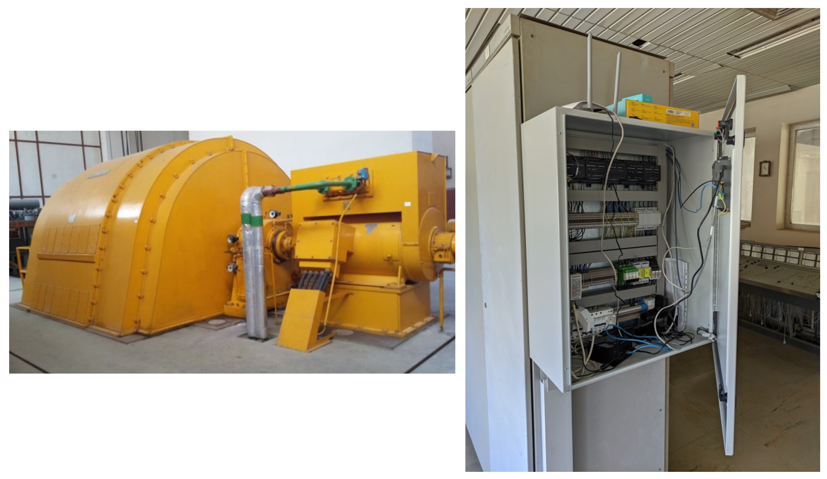
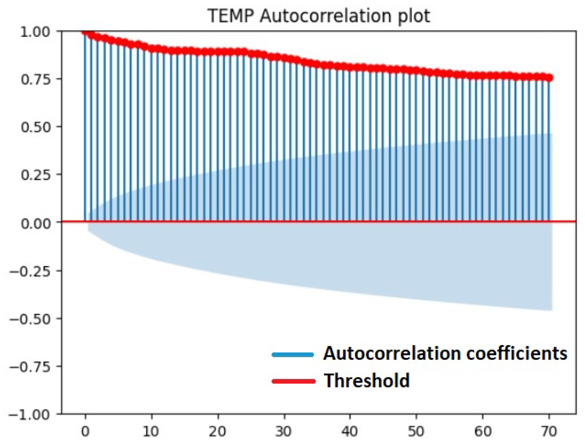
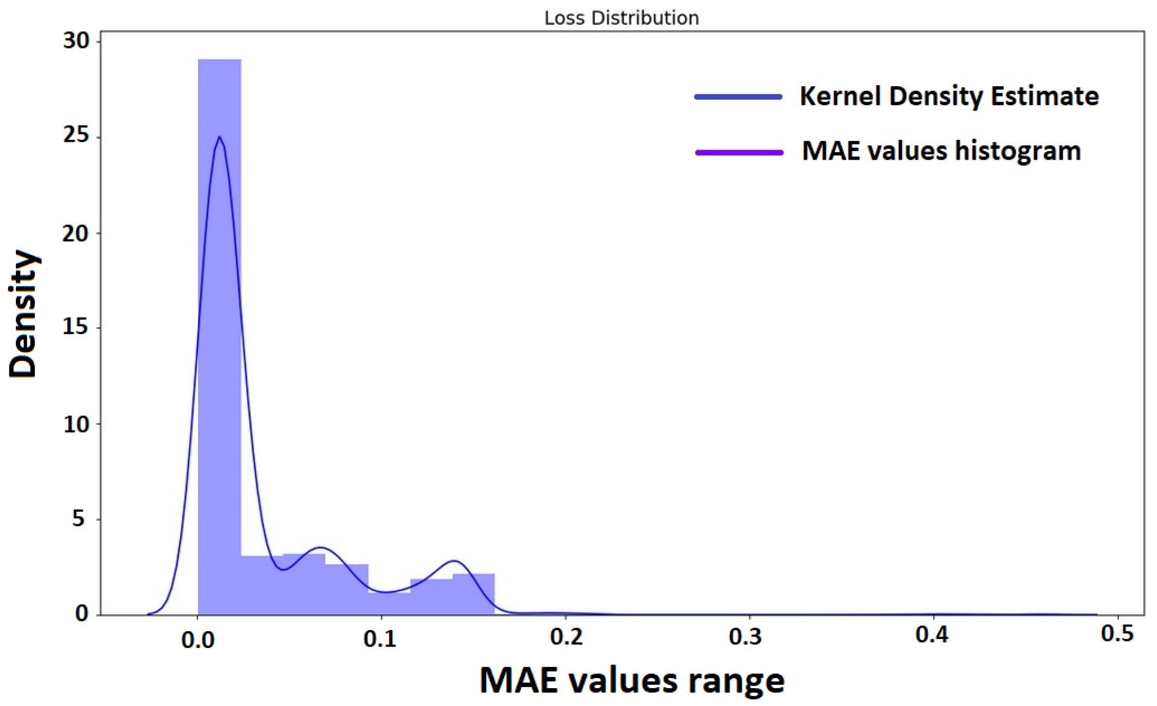
Table 1.
Comparative results of XGBOOST for FH = 1, 2, 20.
| XGBOOST | |||||||
|---|---|---|---|---|---|---|---|
| Feature | RMSE | MAE | MSE | MAPE | SMAPE | R-Squared | Execution Time (s) |
| FH = 1 | |||||||
| CPU_USAGE | 16.081562 | 9.700686 | 258.616642 | 0.802285 | 0.584453 | 0.031290 | 8.310523 |
| MEM_USAGE | 1.034193 | 0.176332 | 1.069555 | 0.006980 | 0.006310 | 0.927815 | 5.695299 |
| TEMP | 1.340489 | 0.448495 | 1.796911 | 0.015917 | 0.016448 | 0.703249 | 5.633248 |
| FH = 2 | |||||||
| CPU_USAGE | 16.002779 | 9.632965 | 256.088941 | 0.799449 | 0.580069 | 0.040758 | 7.252350 |
| MEM_USAGE | 1.503786 | 0.281199 | 2.261373 | 0.011225 | 0.009777 | 0.847379 | 6.215471 |
| TEMP | 1.729988 | 0.742301 | 2.992858 | 0.027374 | 0.028026 | 0.505744 | 5.150763 |
| FH = 20 | |||||||
| CPU_USAGE | 16.359582 | 9.910116 | 267.635921 | 0.801527 | 0.598313 | −0.002494 | 7.562836 |
| MEM_USAGE | 4.198917 | 1.677488 | 17.630903 | 0.067008 | 0.055366 | −0.189915 | 6.721824 |
| TEMP | 3.661425 | 3.206860 | 13.406029 | 0.123073 | 0.132476 | −1.213940 | 8.982070 |
Table 2.
Comparative results of LSTM for FH = 1, 2, 20.
| LSTM | |||||||
|---|---|---|---|---|---|---|---|
| Feature | RMSE | MAE | MSE | MAPE | SMAPE | R-Squared | Execution Time (s) |
| FH = 1 | |||||||
| CPU_USAGE | 16.073372 | 9.709294 | 258.353302 | 0.836435 | 0.605460 | 0.032276 | 112.032020 |
| MEM_USAGE | 1.030191 | 0.352668 | 1.061293 | 0.098696 | 0.095972 | 0.928373 | 71.629515 |
| TEMP | 1.638954 | 0.721787 | 2.686171 | 0.1012347 | 0.102347 | 0.556392 | 128.378663 |
| FH = 2 | |||||||
| CPU_USAGE | 16.204136 | 9.708505 | 262.574038 | 0.761380 | 0.582942 | 0.016467 | 347.660933 |
| MEM_USAGE | 1.697829 | 0.961628 | 2.882623 | 0.031552 | 0.030110 | 0.805451 | 78.131862 |
| TEMP | 1.757734 | 0.943940 | 3.089630 | 0.034834 | 0.035762 | 0.489763 | 330.843.088394 |
| FH = 20 | |||||||
| CPU_USAGE | 16.354352 | 9.958240 | 267.464814 | 0.822262 | 0.602185 | −0.001853 | 843.880262 |
| MEM_USAGE | 3.966356 | 2.169013 | 15.731983 | 0.079472 | 0.069425 | −0.061757 | 319.939965 |
| TEMP | 3.687103 | 3.320900 | 13.594732 | 0.127556 | 0.135518 | −1.245103 | 67.485768 |
Table 3.
Comparative results of ARIMA model for FH = 1, 2, 20.
| ARIMA | |||||||
|---|---|---|---|---|---|---|---|
| Feature | RMSE | MAE | MSE | MAPE | SMAPE | R-Squared | Execution Time (s) |
| FH = 1 | |||||||
| CPU_USAGE | 15.592139 | 9.793359 | 243.114811 | 0.758768 | 0.572132 | 0.089356 | 224.088571 |
| MEM_USAGE | 1.029314 | 0.157386 | 1.059488 | 0.006203 | 0.005560 | 0.928495 | 41.088703 |
| TEMP | 1.589654 | 0.501119 | 2.527000 | 0.018194 | 0.018254 | 0.582678 | 14.763636 |
| FH = 2 | |||||||
| CPU_USAGE | 16.383431 | 10.045988 | 268.416812 | 0.754295 | 0.573199 | −0.005419 | 115.935327 |
| MEM_USAGE | 1.505646 | 0.270228 | 2.266971 | 0.010786 | 0.009342 | 0.847001 | 21.665949 |
| TEMP | 1.815535 | 0.667675 | 3.296167 | 0.024418 | 0.024343 | 0.455654 | 8.728107 |
| FH = 20 | |||||||
| CPU_USAGE | 16.295188 | 8.816155 | 265.533143 | 0.518343 | 0.516078 | 0.005383 | 10.434541 |
| MEM_USAGE | 4.198917 | 1.677488 | 17.630905 | 0.067008 | 0.055366 | −0.189915 | 1.958414 |
| TEMP | 2.170193 | 1.560512 | 4.709738 | 0.059187 | 0.061940 | 0.222210 | 0.826459 |
Table 4.
Comparative results for the anomaly detection models.
| Model | Accuracy | Precision | Recall | F1 Score | ROC-AUC |
|---|---|---|---|---|---|
| Isolation Forest | 0.956119 | 0.895522 | 0.3 | 0.449438 | 0.648888 |
| LSTM Autoencoder | 1.0 | 1.0 | 1.0 | 1.0 | 1.0 |
| Convolutional Autoencoder | 0.946865 | 1.0 | 0.11 | 0.198198 | 0.555 |
| DBSCAN | 0.998507 | 0.975609 | 1.0 | 0.987654 | 0.999206 |
Disclaimer/Publisher’s Note: The statements, opinions and data contained in all publications are solely those of the individual author(s) and contributor(s) and not of MDPI and/or the editor(s). MDPI and/or the editor(s) disclaim responsibility for any injury to people or property resulting from any ideas, methods, instructions or products referred to in the content. |
© 2024 by the authors. Licensee MDPI, Basel, Switzerland. This article is an open access article distributed under the terms and conditions of the Creative Commons Attribution (CC BY) license (https://creativecommons.org/licenses/by/4.0/).
Share and Cite
MDPI and ACS Style
Lekidis, A.; Georgakis, A.; Dalamagkas, C.; Papageorgiou, E.I. Predictive Maintenance Framework for Fault Detection in Remote Terminal Units. Forecasting 2024, 6, 239-265. https://doi.org/10.3390/forecast6020014
AMA Style
Lekidis A, Georgakis A, Dalamagkas C, Papageorgiou EI. Predictive Maintenance Framework for Fault Detection in Remote Terminal Units. Forecasting. 2024; 6(2):239-265. https://doi.org/10.3390/forecast6020014
Chicago/Turabian StyleLekidis, Alexios, Angelos Georgakis, Christos Dalamagkas, and Elpiniki I. Papageorgiou. 2024. "Predictive Maintenance Framework for Fault Detection in Remote Terminal Units" Forecasting 6, no. 2: 239-265. https://doi.org/10.3390/forecast6020014