Estimation of Acoustic Power Output from Electrical Impedance Measurements


1
Faculty of Information Technology and Bionics, Pázmány Péter Catholic University, 1083 Budapest, Hungary
2
Department of Engineering Science, Institute of Biomedical Engineering, University of Oxford, Oxford OX3 7DQ, UK
*
Author to whom correspondence should be addressed.
Acoustics 2020, 2(1), 37-50; https://doi.org/10.3390/acoustics2010004
Submission received: 19 November 2019
/
Revised: 27 January 2020
/
Accepted: 28 January 2020
/
Published: 4 February 2020
(This article belongs to the Special Issue Acoustical Materials)
Abstract
:A method is proposed for estimating the acoustic power output of ultrasound transducers using a two-port model with electrical impedance measurements made in three different propagation media. When evaluated for two high-intensity focused ultrasound transducers at centre frequencies between 0.50 and 3.19 MHz, the resulting power estimates exceeded acoustic estimates by 4.5–21.8%. The method was shown to be valid for drive levels producing up to 20 MPa in water and should therefore be appropriate for many HIFU (high-intensity focused ultrasound) applications, with the primary advantage of employing relatively low-cost, non-specialist materials and instrumentation.
1. Introduction
1.1. Motivation and Overview of Current Methods
The measurement of transducer acoustic output is necessary for deriving safety indices for diagnostic ultrasound transducers; for a review, see [1]. Acoustic power measurements are also critical for therapeutic treatment scenarios, especially those involving targeted hyperthermia [2]. In the current practice, parameters defining safety (peak rarefaction pressure, spatial-peak temporal-average intensity, temporal-average acoustic power) are determined usually by using either a hydrophone measurement system (for pressure and intensity measurement and sometimes also for acoustic power calculations) or a radiation force balance (for acoustic power measurement) [1,3]. However, there are several drawbacks for using hydrophone systems, such as the difficulty in measuring high pressures (they generally do not withstand high pressures and/or long pulses) and the time for the setup of field scans required for power calculation. Measurements using a radiation force balance are much more time efficient; however, the specific-purpose devices are relatively expensive (7–24k USD) and therefore unobtainable by many laboratories and institutes with a limited budget. A method of rapidly testing transducers in a cost-effective manner, using otherwise multi-purpose standard laboratory equipment, may be useful in several use cases. Custom-designed transducers may be quickly tested during production without requiring a full characterization. Moreover, during manufacturing, all manufactured items may be tested without the need for random sampling. Lastly, a clinician may test the performance of a transducer over time without requiring access to expensive equipment.
1.2. Equivalent Circuit Models for Transducers with Reference to the Current Work
The total power dissipation of a transducer is partially due to electrical losses. Calculating the total power dissipation from electrical impedance measurements may provide an upper limit to the acoustic power output, under the assumption that all electrical power going into the transducer is converted to acoustic power. Since such an assumption is too idealistic and leads to a significant overestimation of the acoustic power output of a transducer, more sophisticated methods are needed for a closer estimation of the electrical losses and acoustic output. There exist methods using equivalent circuit models of transducers for a full description of their electrical and acoustical behaviour [4,5], the most popular transducer model being the KLM model [6]. However, these methods require extensive knowledge of transducer parameters (such as physical dimensions, acoustic impedance, sound velocity, and the coupling factor of the piezoelectric ceramic) [7] that are not necessarily available when testing. There also exists work, broadly termed the electromechanical impedance technique, that seeks to characterize a material placed on a piezoelectric transducer by measuring the electrical impedance of the two; for a review, see [8]. However, the aim of such work is not to characterize the power output of the transducer itself, but to characterize the loading placed in front of it.
Here, we propose a method for acoustic output power estimation based on ultrasound transducer electrical impedance measurements only. The transducer is modelled as a two-port network loaded by the acoustic propagation medium, a generalization of the KLM model that retains the linearity and reciprocity assumptions of the latter [7]. Such a lumped two-port model has been used in the literature for electrical matching [9]. Here, the two-port network model parameters are derived by measuring the electrical impedance of the transducer as it is placed in different propagation media (similarly to [10], where the model parameters are used to characterize the properties of a material placed onto the front of the piezoelectric transducer). In the present case, the model parameters are used to estimate the acoustic power dissipation and subsequently compare with acoustic measurements for validation. To the knowledge of the authors, this is the first time that changing the exterior loading of a piezoelectric transducer has been used to estimate its output power.
2. Theory
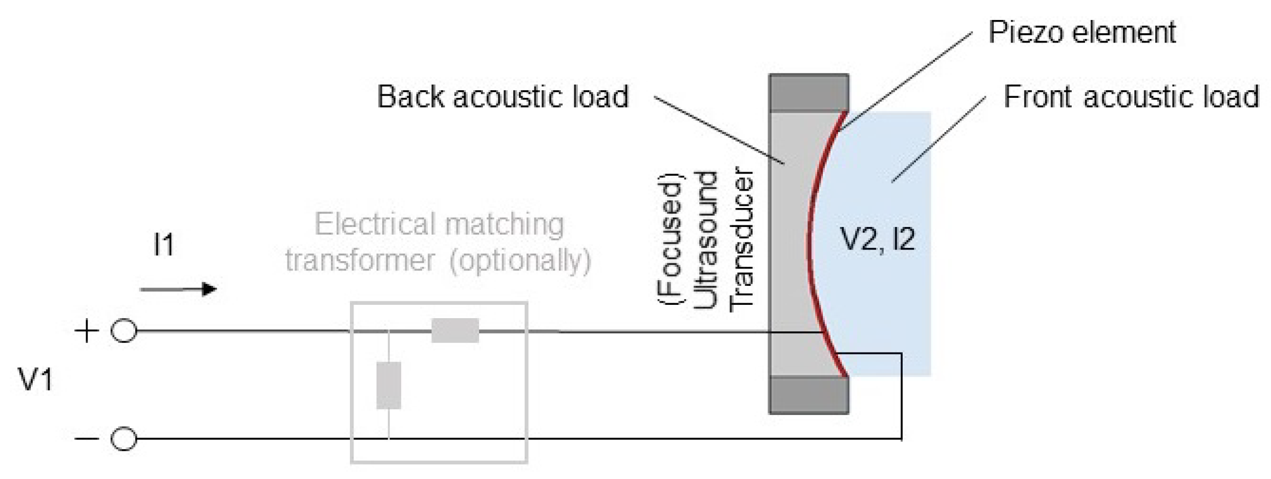
In accordance with the KLM model, a piezoelectric transducer is interpreted as a system with three ports. One electrical port connects the transducer to the electrical pulser and signal receiver system. Two acoustic ports represent the connection to the mechanical fields in the front and back acoustic loads (see Figure 1). In such a model, and stand for the acoustic pressure and particle velocity of the front load, as electrical circuit equivalents. Treating the transducer as a system including the backing load, as well as optional electrical matching circuit as inner parts of the system, the model can be generalized to a two-port network (see Figure 2).
2.1. Two-Port Transducer Model
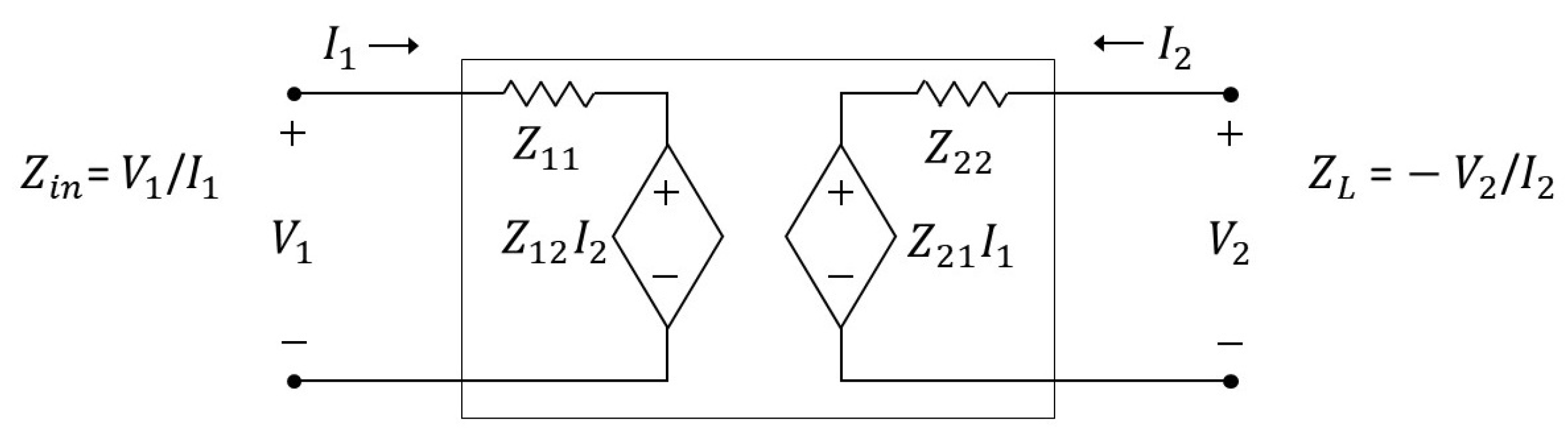
Defining an electrical port as a pair of terminals with equal currents flowing in and out, an electrical circuit with two ports may be treated as a two-port network (Figure 2) defined fully by four impedance parameters [11,12], with state equations:
where , are the voltage at and current going into ports , respectively (with () impedance parameters describing their interconnections). Placing an acoustic load at port 2, the input impedance “seen” from port 1 is [13]:
2.2. Estimation of Two-Port Parameters and Power
The system of equations in Equation (4) is currently not unique for the four impedance parameters of x (Equation (5)). However, using the assumption of reciprocity, generally true for circuits containing passive elements only and shown to be true for the KLM model [7], . During the calculation of the impedance parameters, the square root of is taken, which gives a positive real impedance value for both and . Since there are three unknown terms remaining in x, at any given frequency, measurements of the input impedance using at least three different acoustic loads allows an estimate of the parameter vector to be obtained using matrix inversion. The equation system will have a unique solution as long as the impedance properties of the three loads are different.
Expressing all voltages in terms of their root mean squared (rms) value, the average power dissipated on the acoustic load is:
We note here that the acoustic load in the electrical circuit encapsulates all the acoustic dissipation into the acoustic medium, while the purely electrical dissipation is contained in the two-port network. We further note that can be defined as any multiple of the acoustic impedance, with the two-port network ensuring the appropriate conversion between electrical and acoustic impedance. For simplicity, the acoustic load used is simply the acoustic impedance. The above considerations are analogous to the ones made in the KLM model [7], although our proposed model has a more general and therefore simplified form.
3. Materials and Methods
In this section, we describe the experiments conducted to assess the validity of the proposed method. First, electrical impedance measurements were made with two high-intensity focused ultrasound (HIFU) transducers loaded in turn with three distinct fluid media. Data collected from these measurements were processed according to Section 2.2 to yield estimates of radiated power. Acoustic field measurements were then made in the focal planes of the HIFU transducers in order to gain independent estimates of radiated power. Finally, the pressure range of applicability was assessed through a series of additional acoustic and electrical measurements performed with drive levels producing pressures up to approximately 20 MPa. Details are provided in the following subsections.
3.1. Transducers Used for the Measurements
Two spherically-focused HIFU transducers (Sonic Concepts, Bothell, WA, USA) were used for measurements at both their fundamental and 3rd harmonic frequencies: H-102, SN: B-022 (1.060/3.190 MHz) and H-107, SN: 031 (0.5/1.7 MHz). The fundamental and 3rd harmonic bandwidths, as defined by the manufacturer, down to -3dB normalized to a perfect 50 match, were 640/700 kHz (H-102) and 340/80 kHz (H-107). The H-102 and H-107 transducers had a rectangular and circular cutout, respectively, modifying their surface areas from 32.2 to 26.5 cm and 32.2 to 30.8 cm, respectively (Figures 4a and 5a).
For experimental validation of the theory presented in Section 2, the acoustic power dissipation was estimated from electrical impedance (“Z”) measurements and compared with the corresponding acoustic measurements (acoustic power dissipation calculated from measurements of pressure “p”) as a reference (Figure 3), as described in the following subsections. These measurements were performed for both transducers with both of their driving frequencies.
3.2. Electrical Impedance Measurements
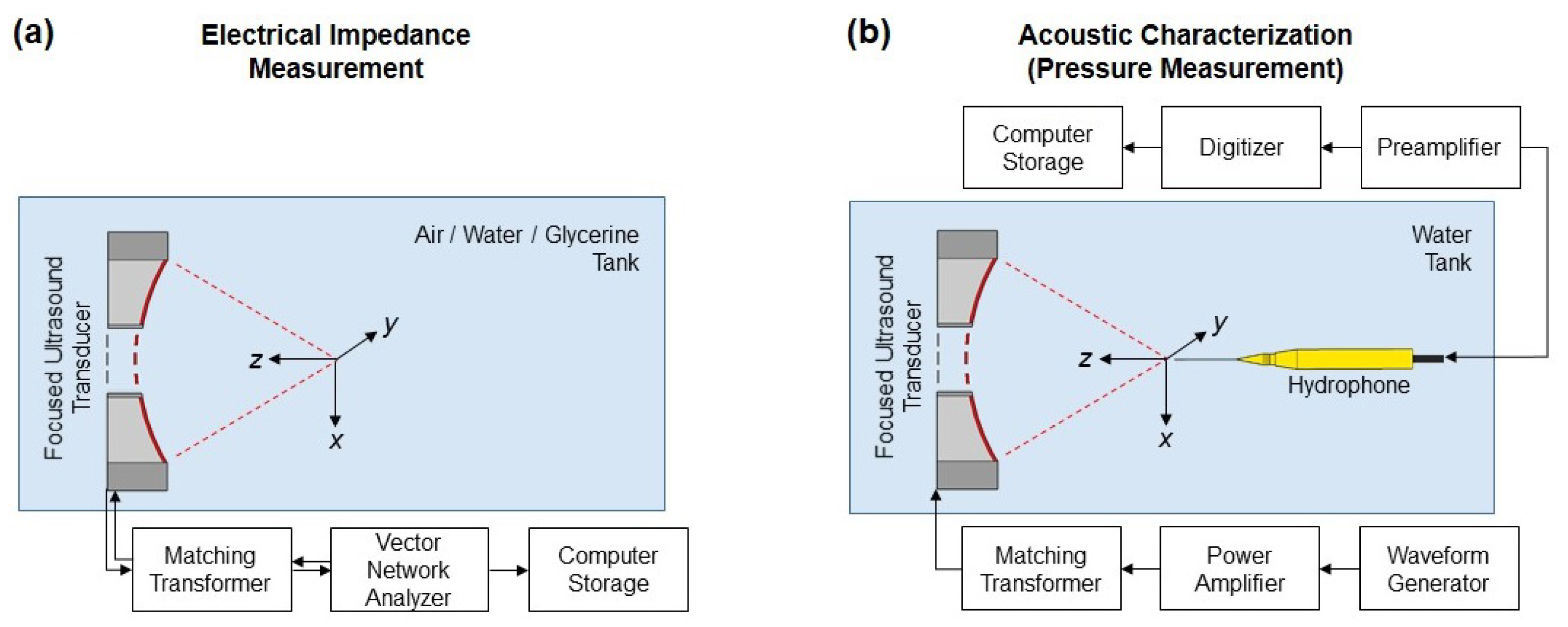
Electrical impedance measurements were performed using a Bode 100 vector network analyser (Omicron Lab, Klaus, Austria), in the frequency range of 100 Hz–4 MHz. The input signal source for the impedance measurements was a continuous wave sinusoid, and a 1 kHz receiver bandwidth was used. Each HIFU transducer had a matching transformer; all electrical measurements were made at the transformer input (Figure 3a). During the measurements, the transducer was placed into three easily obtainable and safe media with known acoustic impedances: air, water, and 87.5% glycerine, with characteristic acoustic impedances of 0.4 , 1.50, and 2.06 MRayl ( Rayleigh) assuming linear mixing for glycerine [14]. Since inadvertent physical movement of the transducer cable could potentially change its impedance, care was taken to not move it while the propagation media was being changed.
The acoustic power output was estimated from the impedance measurements with MATLAB (MathWorks, Natick, MA) using the proposed method (Section 2). For more details on the calculations, see Appendix B. Since the two-port model automatically adapts to the conversion factor used, for simplicity, a conversion factor of 1 was used when defining the load impedances .
The estimated impedance coefficients were used to derive acoustic power consumption, as well as total power consumption for unit peak drive voltage ( V) with water as the acoustic load. Total power consumption was calculated using the first part of Equation (7) for the root mean squared drive voltage and for the impedance of the whole system with water load (as observed from port 1 of the network model) , as follows: . In a similar way, transmitted acoustic power was calculated from the root mean squared output voltage of the two-port network model (see Equation (6)) and from the impedance of water as the load material (). The efficiency of the transducer at a given frequency was calculated as the ratio of the transmitted acoustic power () and the total power (), in %.
3.3. Acoustic Characterization
Direct measurements of radiated acoustic pressure were carried out with the transducers submerged in a tank filled with filtered and degassed water. For each transducer/frequency combination, a drive signal was provided by a waveform generator (Agilent 33225A, Santa Clara, CA, USA) connected to a power amplifier (Model 1140LA, E&I limited, Rochester, NY, USA) as shown in Figure 3b. The drive signal consisted of two-cycle bursts having a centre frequency defined by the manufacturer at the fundamental or third harmonic resonance of the transducer, with the short burst typically providing at least 300 kHz of usable processing bandwidth. Note that due to the capture of both magnitude and phase spectra of the drive and receive waveforms, the output for an arbitrary pulse frequency (within the measurement bandwidth) and length can be reconstructed from these measurement results (see Appendix C), provided that the longer pulse length itself does not introduce additional nonlinearities (e.g., near a cavitation threshold). The focal plane pressure fields were measured with a calibrated needle hydrophone (HNC0400, (Onda Corp, Sunnyvale, CA, USA) for 500 kHz, or PA0200 (Precision Acoustics, Dorset, U.K.) for higher frequencies). Hydrophone positioning and data acquisition were coordinated by software control (UMS, Precision Acoustics). Spatial measurement ranges were chosen to capture at least three sidelobes, as verified by preliminary line scans. Additional measurements were made on the H-107 transducer at higher amplitudes and varying pulse lengths in order to assess the validity of the proposed power estimation method with respect to drive scaling and system linearity.
For estimates of radiated power, the point-by-point field measurements were first Fourier transformed and normalized by the transform of the drive voltage and the hydrophone calibration to yield pressure spectra per unit drive voltage:
Radiated power was then found by numerically integrating the pressures under the assumption of locally planar propagation:
where the integration area was taken from the scan step size (0.1 mm) and the ambient sound speed c was found from a temperature-speed relationship [15] and a thermocouple measurement made during the scan.
It should be noted that the H-107 measurements were repeated to expand the spatial scan for power computation. In the time between the initial and repeat experiments, it was found that the electrical impedance of the H107-matching transformer system changed. This was accounted for using the procedures in Appendix D.
3.4. Measurements Validating the Range of Linearity for the Model
The estimate of acoustic power output from a given voltage input relied on a linear model. The electrical impedance measurements were done using a small current injection so their linear extrapolation should work as long as the acoustic output was in the linear range. To demonstrate the validity of linearity in terms of drive voltage, measurements were performed as follows.
The H-107 transducer was driven in its 3rd harmonic band over a range of amplitudes so that the final peak to peak pressure was just over 20 MPa. Fields were measured with a membrane hydrophone (D1602, Precision Acoustics, Dorset, U.K.) whose frequency response was flat within 1–2% over the 1–20 MHz range allowing determination of calibrated pressure as harmonics appeared in the received waveforms. The hydrophone was scanned through a radial line spanning ±6 mm about the focus for each drive level, and the scan data were processed to yield acoustic power estimates as described above (Equation (9)). Electrical impedance was also measured, using a current probe (4100, Pearson Electronics, Palo Alto, CA, USA) and a voltage probe (PP017, LeCroy, Geneva, Switzerland) connected to the amplifier output.
4. Results
4.1. Comparison of Estimated and Measured Acoustic Powers
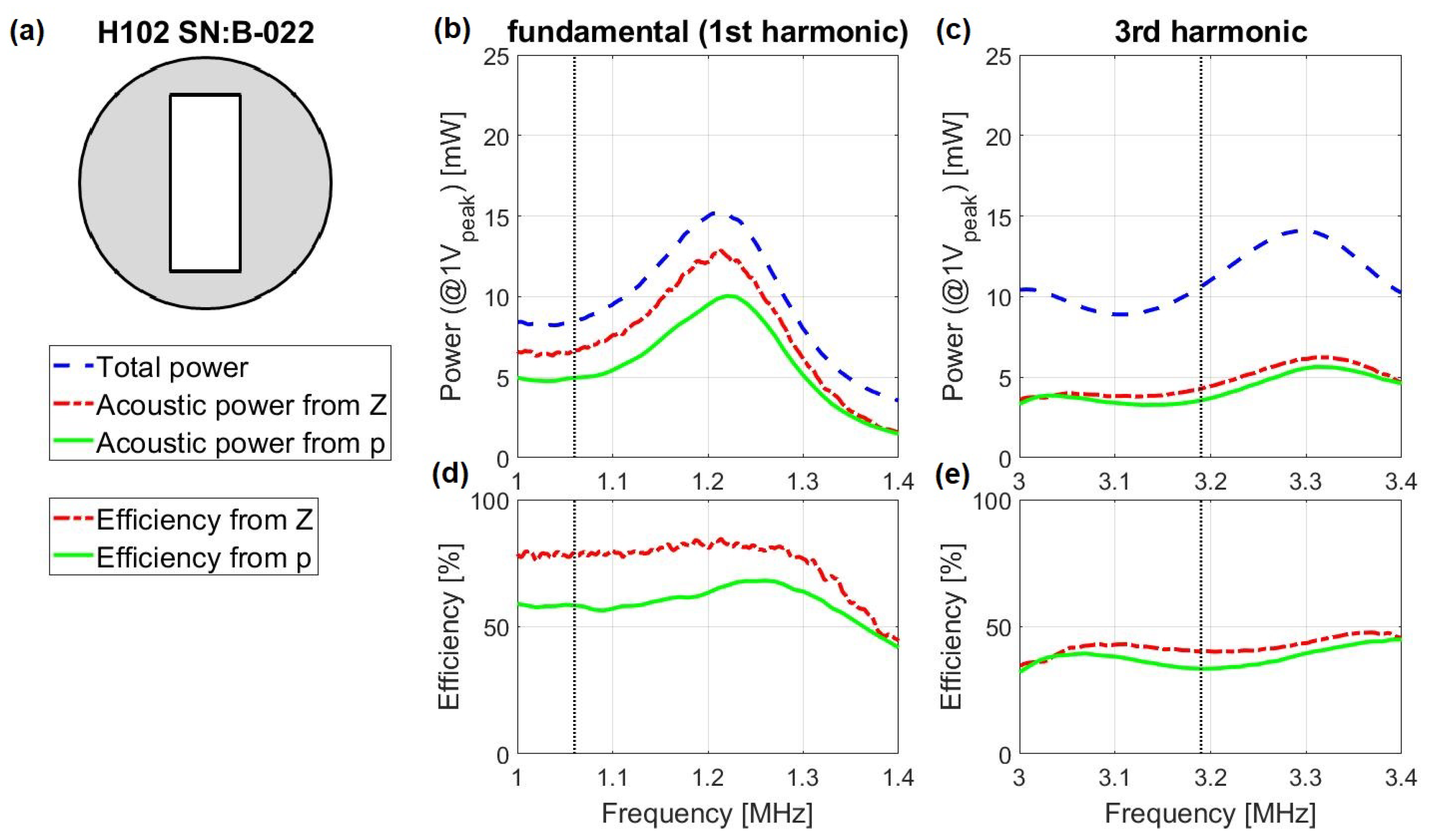
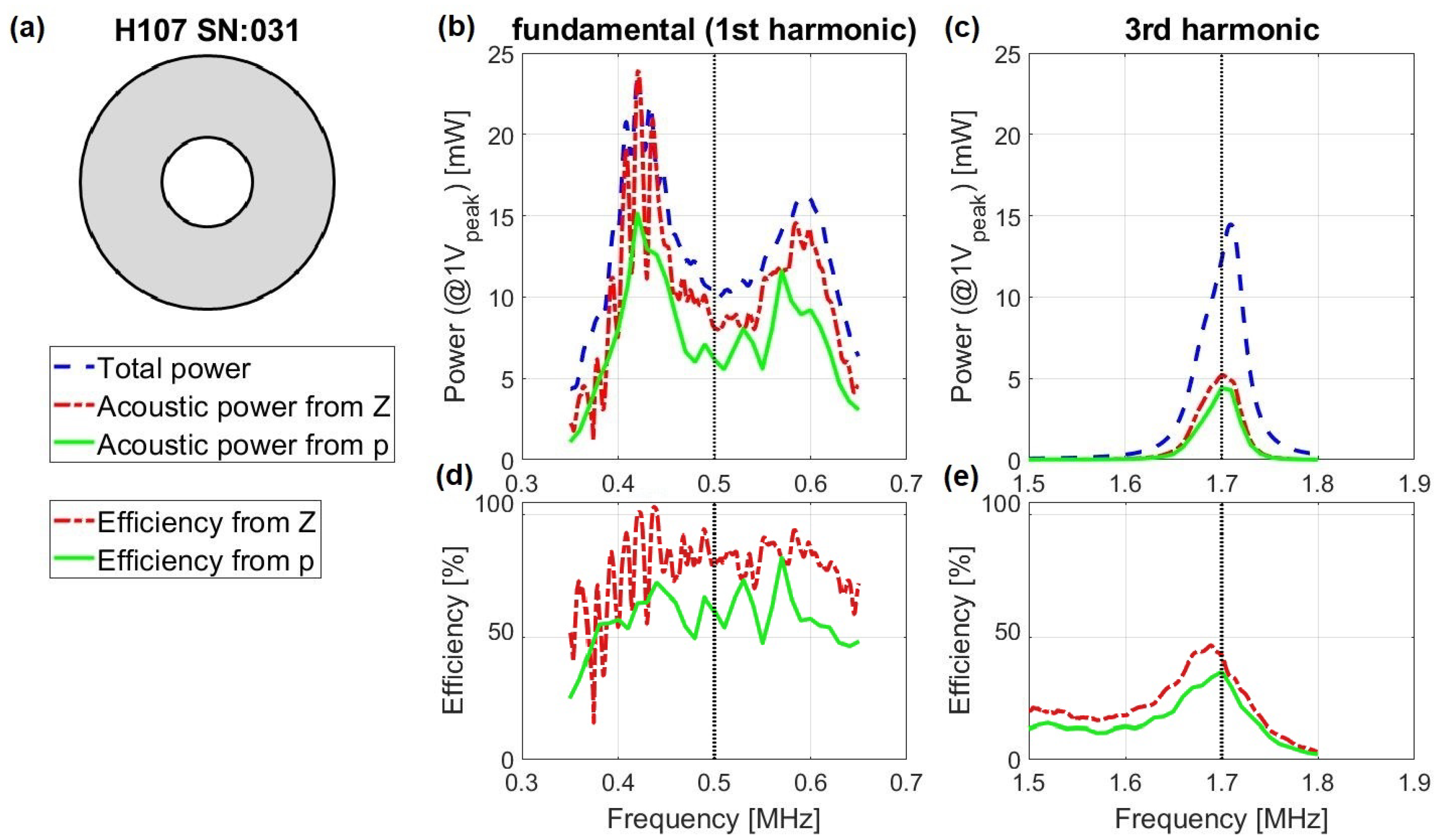
Results are shown here in terms of power and efficiency. As an example, in Figure 4, the estimated (from impedance “Z”) and measured (from pressure “p”) acoustic powers were compared in relation to the total (electric and acoustic) power calculated from impedance measurements (Section 3.2). The lower plots (d,e) show the efficiency calculated for both estimation and measurement of acoustic power, using the data of the plots at the top (b,c).
The results for four cases of transducer and driving frequency combinations (see Figure 4 and Figure 5) indicated that the method presented in this paper gave an estimation in between the total power and the measured acoustic power values. A good agreement was found in the frequency dependency of these three values, with estimations being closer to the measured acoustic power for frequencies near the third harmonic, coupled with a lower efficiency. At the nominal transducer resonance frequencies, the estimated/measured powers were 6.7/5.0 mW (H-102, 1.06 MHz) 4.3/3.6 mW (H-102, 3.19 MHz), 8.1/6.2 mW (H-107, 0.5 MHz), and 5.2/4.4 mW (H-107, 1.7 MHz). The mean absolute difference between estimated and measured power, in % of the average measured power, was 17.0% and 4.5% for the H-102 fundamental and third harmonic; 21.8% and 7.8% for the H-107 fundamental and third harmonic. The impedance-based power predictions were consistently above the acoustic measurements. The acoustic measurements themselves had an uncertainty of around 32% (in accordance with 15% hydrophone calibration uncertainty for pressure). The uncertainty of the impedance-based method was estimated to be between 0.7 and 7.1% depending on the device and its drive band (Appendix E).
4.2. Linearity of the Model
The linearity of the transducer response, in terms of pressure-voltage correlation, was assumed when suggesting that the small-signal impedance measurements used to estimate the power output of the transducer were valid over a higher voltage range, as well as for a broad frequency range.
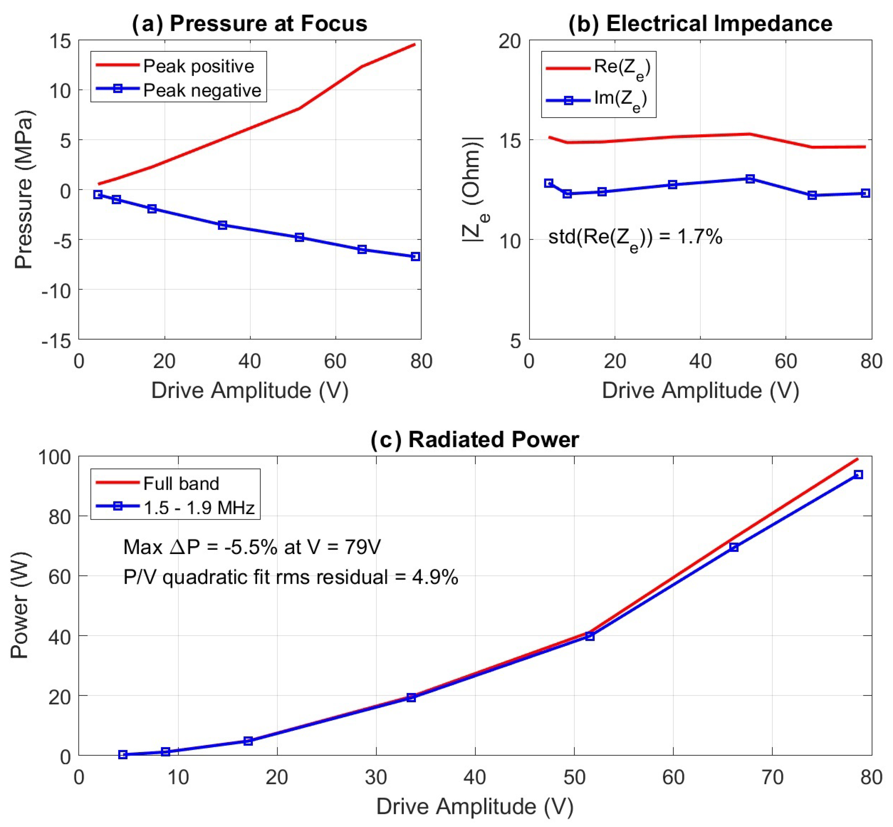
A wide range of linearity was verified for the proposed model by measurements performed as described in Section 3.4. Results are shown in Figure 6.
Figure 6a shows the peak positive and negative pressures measured at the focus of the H-107 transducer and includes all frequency content up to 20 MHz. From the asymmetry of the values, the waveform clearly exhibited nonlinear behaviour even at low drive levels (“drive amplitude” is the amplifier output).
Figure 6b shows the values of electrical impedance at 1.7 MHz as determined from voltage and current probes at the amplifier output terminal. The datasets had standard deviations of <2% over the drive range. At the higher drive levels, small nonlinearities did show up in the drive spectrum (not shown on the figure), but they were no larger than 1/20th of the 1.7 MHz amplitude. All this suggested that the nonlinearities were primarily in the water, not in the drive chain (as expected). Because the electrical impedance was essentially invariant with driving amplitude, this further validated the use of the proposed model for higher driving voltages.
In Figure 6c, the computed radiated powers are shown in two forms: using the full bandwidth of the data and only keeping the part that was in the 1.5–1.9 MHz band. The latter presumably was what would come from the electrical impedance-based predictions. At the highest drive level, the band-limited power estimate was only 5.5% lower than the full band. This was largely as expected when the nonlinearity was occurring locally in the focus due to elevated pressures. The main lobe peak had a minimal contribution to the total power because there was very little corresponding area through which energy flowed at the peak intensity. For pressures in the range reported here, similar observations were made regarding heating of tissues with focused beams: nonlinearity may produce a waveform distortion, but it did not necessarily impact spatially cumulative outputs that were quadratic in pressure (e.g., power, heat deposition). Finally, the power–voltage curves followed the expected quadratic dependence, with a residual difference of about 5%.
In summary, the proposed method did not appear to be limited by deviations from linearity (or voltage scaling as presented above) for this transducer for up to 20 MPa peak-peak pressure. This pressure range is relevant to many therapeutic scenarios, and therefore, the association with “HIFU” is appropriate based on these findings.
5. Discussion
5.1. Interpretation of Transducer-Specific Phenomena Affecting Measurements
As shown in Figure 4 and Figure 5, efficiency values at the fundamental frequency were significantly lower for measured acoustic power than for electrical impedance-based estimations, in all four cases. The efficiency estimates were also lower than the values reported by the manufacturer for a representative transducer (with different SN). However, the representative transducer did not have a cutout, and having cutouts of any shape (and the resulting boundary conditions and vibration shapes) could impact the power estimates via the input energy going into subsonic vibrations (such as bending or surface wave motion) near the edges of the ceramic, rather than deformation that produces volume change and efficient radiation. In this way, some energy may be dissipated in ceramic losses and kinetic energy of the loading fluid (water), near the edges. Assuming that the edge “losses” scale with the wavelength may explain the larger difference between estimated and measured acoustic power for the fundamental frequency than that for the third harmonic.
Conceivably, a larger transducer with a greater surface area to edge length would be less susceptible to the proposed loss mechanism. To the authors’ knowledge, all clinical HIFU transducers (unless array based) would fit this description. Another potential loss mechanism at lower frequencies would be coupling into the transducer body (side walls). In a transducer without a cutout, we would expect even closer correspondence of our impedance-based estimates of the acoustic power dissipation with the real dissipation shown by reference acoustic measurements.
The acoustic resonance frequencies, as measured using electrical impedance and acoustic measurements, are seen to be in close agreement in Figure 4 and Figure 5. However, there were discrepancies with the values provided by the manufacturer. This could be due to several factors, including changes of transducer properties with time and handling.
5.2. Scaling of the Results
The results presented in Section 4.1 were measured and calculated for unit voltage amplitude. Projections to a given drive voltage amplitude should consider both the electrical and acoustic linearity of a specific transducer for a drive voltage and frequency range. Note that, with the assumption of linearity, the power output increased as the square of voltage (meaning that a 32 V drive would scale the plots of Figure 4 and Figure 5 from mW to W), and for HIFU applications, even higher voltages (e.g., 50 V and higher) were typically used. As long as the model was applied in its linear range, the relative (%) errors (Section 4.1) remained valid.
The effect of drive level on the scaling of model results was evaluated with the H-107 transducer, with measurements made of the drive voltage, drive current, and focal plane acoustic pressure (Section 4.2). For drive amplitudes between 4 and 79 V, the electrical impedance in the “drive band” (1.6–1.8 MHz) exhibited negligible variation (1.7% standard deviation). At the highest drive amplitude, the focal pressure waveform was highly nonlinear, with a peak-to-peak value of approximately 20 MPa. Still, the estimated radiated power followed a simple quadratic relationship with drive voltage over the range tested. This presumably was because the amplifier-transducer system behaved linearly, and the nonlinear response of the medium (water) was not strong enough to cause meaningful thermo-viscous losses that would appear as a loss of beam power. Further study would be required to evaluate other transducer systems and drive conditions. However, the data in this study confirmed that the proposed method was valid even when the response of the medium yielded strongly nonlinear waveforms.
5.3. Potential Advantages of the Proposed Method
The primary advantage of the proposed method is its cost effectiveness. The liquids used for the presented measurements are commonly available lab supplies, and the electrical impedance measurement could be done with probes or simple circuits if an impedance analyser were not available. Another advantage is its simplicity. It only requires changing the media in which the transducer is placed and performing quick impedance measurements in each. There is no need for precise setting of the orientation of the transducer if the tank is large enough. A further advantage is time effectiveness. An electrical impedance measurement only takes about a few seconds for a frequency range of tens of MHz. Including the changes of propagation media, the three measurements can be done within 15 min, approximately.
Future work could investigate the use of media with an even higher acoustic impedance than glycerine to ensure a higher contrast in electrical impedance values, the expected effect being to reduce sensitivity to measurement errors.
6. Conclusions
A method for acoustic power output estimation of ultrasound transducers was proposed in this paper, based on simple electrical impedance measurements in three different propagation media and requiring knowledge only of the relative characteristic acoustic impedances of these media. Results showed agreement of estimated acoustic power outputs (based on electrical measurements) with relevant reference acoustic measurements, for four cases of transducer and driving frequency combinations. Since the estimates were consistently above the measured acoustic values, they may potentially be useful for providing an upper bound for ultrasound exposure safety analyses. Quantitatively, a 21.8% overestimate as seen with the H-107 fundamental would translate to a 10.4% overestimate in pressure, which is similar to the maximum uncertainty in a direct measurement with a hydrophone. Drive scaling analyses indicated that the proposed method could yield valid power estimates even when the output waveform was highly nonlinear, making it suitable for many HIFU calibration scenarios.
Although estimates of acoustic power dissipation may be used to estimate acoustic intensity and pressure output, this was left out of the scope of the current paper as the calculations involved considerable deliberation [2]. However, with future work, the proposed time-, complexity-, and cost-effective method may be elaborated to give predictions on the mechanical index (MI) and thermal index (TI) used to characterize ultrasound transducer safety for diagnostic and therapeutic applications. Such a method would be of great benefit for making quick and simple independent measurements both in industrial and clinical environments, filling a gap for laboratories and institutes with a limited budget.
Author Contributions
Conceptualization, M.G.; methodology, software and validation, G.C., M.D.G., and M.G.; writing, original draft preparation, G.C.; writing, review and editing, M.D.G. and M.G. All authors have read and agreed to the published version of the manuscript.
Funding
This research was funded by Pázmány Péter Catholic University Grant Numbers KAP15-054-1.1-ITK and KAP16-71005–1.1-ITK. The APC was funded by Pázmány Péter Catholic University.
Acknowledgments
The experiments were carried out in the BUBBL (Biomedical Ultrasonics, Biotherapy and Biopharmaceuticals Laboratory) lab (at the Institute of Biomedical Engineering, Department of Engineering Science, University of Oxford, Oxford, U.K.). The authors thank the generosity of Constantin-C. Coussios for use of laboratory equipment. The authors further thank Jeffrey Ketterling, Dan Gross, and Balázs Bajnok for help with measurements and theory and Árpád I. Csurgay for discussions on electrical theory.
Conflicts of Interest
The authors declare no conflict of interest. The funders had no role in the design of the study; in the collection, analyses, or interpretation of data; in the writing of the manuscript; nor in the decision to publish the results.
Abbreviations
The following abbreviations are used in this manuscript:
| HIFU | High-intensity focused ultrasound |
| KLM model | Equivalent circuit model of piezoelectric ultrasound transducers, named after R. Krimholtz, D. A. Leedom and G. L. Matthaei |
Appendix A. Derivation of Equation (6) from Equations (1) and (2)
In order to express voltage in terms of voltage and impedance parameters of the two-port network, first, we want to eliminate currents and from the expressions. Rearrangement of Equation (A1) yields:
while a similar rearrangement of Equation (A2) yields:
Rearrangement of Equation (A6) leads to:
Using this expression for (Equation (A7)), Equation (A3) becomes:
Appendix B. Calculation of the Two-Port Network Parameters
As discussed in Section 2, the two-port network parameters (Figure 2) can be calculated by solving the set of linear equations Equation (4) for (defined in Equation (5)).
Impedance measurements using three different materials (a, w, g) for load provide an equation system of three equations as follows (according to Equation (4)):
where are impedances measured using the load material m and are the characteristic acoustic impedances of the material m ().
From the equation set (of three equations for three materials), the parameter vector was calculated using matrix inversion. Parameters of the two-port network model were then calculated from the parameter vector defined by Equation (5) and by using the assumption of reciprocity: .
Appendix C. The Validity of Short-Pulse Measurements for HIFU Transducers
The input-to-output transfer function of a linear system should be independent of the particular form of the input (e.g., impulsive or tonal), provided that the data have adequate recording time, spectral overlap, and signal-to-noise ratio. In the particular case of the acoustic measurements in the presented study, the use of a short-pulse drive signal can correctly describe the input voltage to output power transfer function, even though the band of interest involves the resonant response of a transducer. To prove this, the authors recorded drive voltage and focal plane pressure waveforms for the H-107 system when driven with two pulse lengths, both with the same fundamental frequency (0.5 or 1.7 MHz). The transfer function in Equation (8) was then calculated as described in the manuscript, and the ratio of the transfer function magnitudes () was computed. The results are as follows (Table A1).

Table A1.
Comparison of transfer function ratios for the H-107 (SN: 031) transducer system driven with short versus long pulses, in both driving frequencies of the transducer.
Table A1.
Comparison of transfer function ratios for the H-107 (SN: 031) transducer system driven with short versus long pulses, in both driving frequencies of the transducer.
| Drive Band (MHz) | Pulse Lengths (cycles) | Transfer Function Ratio, 200 kHz Band | Transfer Function Ratio, at Centre Frequency |
|---|---|---|---|
| “Fundamental” | 2, 12 | 0.994: 0.4–0.6 MHz | 0.998: 0.50 MHz |
| “3rd Harmonic” | 2, 40 | 0.997: 1.6–1.8 MHz | 0.997: 1.70 MHz |
With the ratios all being within 0.6% of unity, these results clearly validated the approach described in Section 3.3 and further confirmed the handling of the system as one operating in a linear regime.
Appendix D. Scaling of the H-107 Acoustic Measurements after Repetition
Initial measurements of acoustic pressure did not all have sufficiently broad spatial and frequency coverage to calculate radiated power accurately. Upon determining this, the measurements were repeated with a broader spatial and frequency span. However, it was found upon this repeat that the H-107 (SN: 031) matching transformer for the third harmonic frequency band was damaged in the interim. Since the beam patterns (where they overlapped) did not changed, but the response spectrum did, we estimated the H-107 power using a pressure defined by: , where is the original pressure measurement made in the centre of the focal plane and is the focal plane beam pattern made during the repeat measurements. Power was then estimated using Equation (9).
As a consistency check, this process was also done for the fundamental frequency. Comparison of the modified calculation and one made entirely based on the repeat measurements of both pressure and beam pattern showed agreement within 16.73% for the fundamental frequency.
Appendix E. Uncertainty Estimation of the Impedance Measurement-Based Method
The uncertainty of the impedance measurement-based method was estimated based on the uncertainty of the impedance measurements. Multiple (3–8) measurements were performed for each transducer placed in each material (air, water, glycerine). Impedance measurements showed significant accordance. Variability analysis showed the worst-case (biggest) standard variation being 2.91 (0.86% of the highest impedance measured), while the mean standard variation for all frequencies of all measurements for both transducers was 0.18 (0.05% of the highest impedance measured and 2.12% of the average of all impedances measured).
From the impedance measurements, the highest difference from the average was calculated for each frequency of interest, for all four cases of transducer and driving frequency combinations, for all three materials, and for the real and imaginary parts of the measured impedance, separately. The calculated values were used as the standard deviation of the Gaussian random noise added to the relevant impedance measurements (of the measurements presented in the article). Power estimates were calculated, and the uncertainty of the method was estimated as the mean absolute difference of the power estimate using noisy measurement data compared to the power estimate calculated from the noiseless measurement data presented in the article and normalized by the average total power of the latter.
Repeating the above calculation for 1000 different Gaussian random noises, for each transducer and driving frequency combinations, gave the following results. The maximal mean absolute differences of the power estimate from noisy and noiseless measurement data were 1.1%, 0.7%, 7.1%, and 1.7% for transducers and driving frequencies of the H-102 fundamental, H-102 third harmonic, H-107 fundamental, and H-107 third harmonic, respectively.
References
- Shaw, A.; Martin, K. The acoustic output of diagnostic ultrasound scanners. In The Safe Use of Ultrasound in Medical Diagnosis, 3rd ed.; ter Haar, G., Ed.; The British Institute of Radiology: London, UK, 2012; pp. 18–45. [Google Scholar]
- Civale, J.; Rivens, I.; Shaw, A.; ter Haar, G. Focused ultrasound transducer spatial peak intensity estimation: A comparison of methods. Phys. Med. Biol. 2018, 63, 055015. [Google Scholar] [CrossRef] [PubMed]
- Preston, R.C. Output Measurements for Medical Ultrasound; Preston, R.C., Ed.; Springer Science & Business Media: Berlin, Germany, 2012. [Google Scholar]
- Johansen, T.F.; Rommetveit, T. Characterization of ultrasound transducers. In Proceedings of the 33rd Scandinavian Symposium on Physical Acoustics, Geilo, Norway, 9 February 2010. [Google Scholar]
- San Emeterio, J.L.; Ramos, A. Models for piezoelectric transducers used in broadband ultrasonic applications. In Piezoelectric Transducers and Applications, 2nd ed.; Arnau, A., Ed.; Springer: Berlin, Germany, 2009; pp. 97–116. [Google Scholar]
- Krimholtz, R.; Leedom, D.A.; Matthaei, G.L. New equivalent circuits for elementary piezoelectric transducers. Electron. Lett. 1970, 6, 398–399. [Google Scholar] [CrossRef]
- Van Kervel, S.; Thijssen, J. A calculation scheme for the optimum design of ultrasonic transducers. Ultrasonics 1983, 21, 134–140. [Google Scholar] [CrossRef]
- Annamdas, V.G.M.; Soh, C.K. Application of electromechanical impedance technique for engineering structures: Review and future issues. J. Intell. Mater. Syst. Struct. 2010, 21, 41–59. [Google Scholar] [CrossRef]
- Rathod, V.T. A review of electric impedance matching techniques for piezoelectric sensors, actuators and transducers. Electronics 2019, 8, 169. [Google Scholar] [CrossRef] [Green Version]
- Ndiaye, E.B.; Duflo, H.; Maréchal, P.; Pareige, P. Thermal aging characterization of composite plates and honeycomb sandwiches by electromechanical measurement. J. Acoust. Soc. Am. 2017, 142, 3691–3702. [Google Scholar] [CrossRef]
- Hayt, W.H.; Kemmerly, J.E.; Durbin, S.M. Engineering Circuit Analysis; McGraw-Hill: New York, NY, USA, 2002. [Google Scholar]
- Sedra, A.S.; Smith, K.C. Microelectronic Circuits; Oxford University Press: New York, NY, USA, 1998. [Google Scholar]
- Yang, W.Y.; Lee, S.C. Circuit Systems with MATLAB and PSpice; John Wiley & Sons: Hoboken, NJ, USA, 2008; Chapter 10. [Google Scholar]
- Selfridge, A.R. Approximate material properties in isotropic materials. IEEE Trans. Son. Ultrason. 1985, 32, 381–394. [Google Scholar] [CrossRef]
- Marczak, W. Water as a standard in the measurements of speed of sound in liquids. J. Acoust. Soc. Am. 1997, 102, 2776–2779. [Google Scholar] [CrossRef]
Figure 1.
Schematic of a single transducer element system, showing electrical connections, back and front acoustic loading, and electrical matching as an optional part of the network. and stand for the voltage and current at the electrical port of the transducer, while and represent the acoustic pressure and particle velocity of the front acoustic load, seen as a voltage and current, respectively, in the equivalent circuit model.

Figure 2.
Schematic of the two-port network model with impedance parameters . is the load impedance at port 2. The impedance measured at port 1 is .
Figure 2.
Schematic of the two-port network model with impedance parameters . is the load impedance at port 2. The impedance measured at port 1 is .

Figure 3.
Schematic of the (a) electrical impedance measurements (Section 3.2) and of the (b) acoustic characterization (pressure measurements from which acoustic power was calculated; see Section 3.3).
Figure 3.
Schematic of the (a) electrical impedance measurements (Section 3.2) and of the (b) acoustic characterization (pressure measurements from which acoustic power was calculated; see Section 3.3).

Figure 4.
Comparison of electrically estimated (from impedance “Z” measurements) and acoustically measured (estimated from acoustic pressure “p” field measurements) power outputs (1 V peak drive voltage) of the H-102 (SN: B-022) transducer. (a): Transducer surface schematic with the cutout. (b,c): Total (electric and acoustic) power and estimated and measured acoustic power. (d,e): Estimated and measured efficiency. The dotted vertical lines indicate the centre frequency defined by the manufacturer at the fundamental and third harmonic resonances of the transducer.

Figure 5.
Comparison of electrically estimated (from impedance “Z” measurements) and acoustically measured (estimated from acoustic pressure “p” field measurements) power outputs (1 V peak drive voltage) of the H-107 (SN: 031) transducer. (a): Transducer surface schematic with the cutout. (b,c): Total (electric and acoustic) power and estimated and measured acoustic power. (d,e): Estimated and measured efficiency. The dotted vertical lines indicate the centre frequency defined by the manufacturer at the fundamental and third harmonic resonances of the transducer.

Figure 6.
Validation of the small-signal electrical impedance measurement results to higher driver voltages (resulting in higher pressures and powers). (a) Focal pressure, (b) electrical impedance, and (c) radiated power measurements as a function of drive voltage in the range of 4–80 V showing the linearity of the pressure-voltage correlation, in the case of the third harmonic band (∼1.7 MHz) of the H-107 (SN: 031) transducer.

© 2020 by the authors. Licensee MDPI, Basel, Switzerland. This article is an open access article distributed under the terms and conditions of the Creative Commons Attribution (CC BY) license (http://creativecommons.org/licenses/by/4.0/).
Share and Cite
MDPI and ACS Style
Csány, G.; Gray, M.D.; Gyöngy, M. Estimation of Acoustic Power Output from Electrical Impedance Measurements. Acoustics 2020, 2, 37-50. https://doi.org/10.3390/acoustics2010004
AMA Style
Csány G, Gray MD, Gyöngy M. Estimation of Acoustic Power Output from Electrical Impedance Measurements. Acoustics. 2020; 2(1):37-50. https://doi.org/10.3390/acoustics2010004
Chicago/Turabian StyleCsány, Gergely, Michael D. Gray, and Miklós Gyöngy. 2020. "Estimation of Acoustic Power Output from Electrical Impedance Measurements" Acoustics 2, no. 1: 37-50. https://doi.org/10.3390/acoustics2010004