
A Two-Dimensional Liquid Sloshing Analysis in a Partially Filled Complicated-Shape Tank by the Schwarz–Christoffel Transformation

Department of Dynamics and Control, Beihang University, Beijing 100191, China
*
Author to whom correspondence should be addressed.
Acoustics 2024, 6(2), 346-361; https://doi.org/10.3390/acoustics6020018
Submission received: 7 March 2024
/
Revised: 25 March 2024
/
Accepted: 3 April 2024
/
Published: 19 April 2024
Abstract
:The nonlinear sloshing of an incompressible fluid with irrotational flow in a complicated-shape tank due to horizontal excitation is studied with a semi-analytical method proposed in this study. In this method, the velocity potential function of a liquid in a complicated-shape tank is estimated by using an approximate analytical transformation function from a complicated-shape region to a rectangular region. This function is obtained through Schwarz–Christoffel mapping and polynomial fitting. Nonlinear dynamic equations for the fluid–structure coupled system are developed based on the Hamilton–Ostrogradskiy principle. Nonlinear kinematic equations for the fluid–structure coupled system are derived based on the relationship between the liquid velocity and the free-surface equation. The Galerkin method is used to convert partial differential equations into ordinary differential equations. When tank movement is given, nonlinear models for the coupled system can be reduced to simple ones for liquid sloshing. Natural frequencies for the coupled system and liquid sloshing are analyzed, and the semi-analytical results agree with the numerical ones calculated with the software DampSlosh. Hydrodynamic forces and moments are also analyzed, and the semi-analytical results agree well with the numerical ones calculated with the Flow3D v10.1.1.
1. Introduction
Sloshing is the motion of a liquid in a partially filled container with an unrestrained free surface due to external excitation. Understanding this complicated dynamic behavior is of practical significance, especially when the liquid contributes a non-negligible portion to the total mass, because liquid sloshing is observed in a wide range of engineering applications, such as heavy-duty road tankers, oceangoing vessels, oil tankers, rockets, and aerospace transportation vehicles [1,2,3,4,5]. The primary challenge in sloshing analysis lies in accurately estimating the natural frequencies, hydrodynamic forces, and moments of liquid sloshing. If the excitation frequency is close to natural frequencies, especially the lowest ones, resonance may occur and result in catastrophic consequences. The hydrodynamic forces and moments of sloshing applied to a container may also lead to uncontrollability and structural damage. Furthermore, the containers used in engineering applications are of various shapes, and each individual container shape requires a dedicated applied mathematical and physical study.
Numerous researchers have studied the problem of liquid sloshing, and their research approaches are generally classified as analytical, numerical, and experimental. For analytical approaches, variational formation based on Hamilton’s principle is regarded as the most powerful tool for developing fluid field equations, and the velocity potential function is a key factor in the analytical process. If the fluid motion is irrotational and incompressible, the velocity potential function should satisfy Laplace’s equation. Rectangular coordinates are used to solve Laplace’s equation and the boundary condition on the wetted tank surface for rectangular tanks [6,7,8,9]. Similarly, cylindrical, bipolar, toroidal, and spherical coordinates are used to solve velocity potential functions for upright cylindrical, horizontal cylindrical, annular cylindrical, and spherical tanks, respectively [10,11,12,13,14,15]. However, velocity potential functions can be obtained directly by solving Laplace’s equation and the boundary condition for a limited number of tank shapes only. Conformal mapping can be used to estimate velocity potential functions for other tank shapes because the velocity potential function of liquid sloshing is harmonic. Nevertheless, conformal mapping is mainly applied to only a few tank shapes, such as half-full horizontal elliptical, horizontal circular, horizontal cylindrical, and spherical, to determine the velocity function of fluid [16,17,18,19,20,21]. The nonconformal transformation technique and the variational modal approach have been developed for circular conical and prolate spheroidal tanks; one scheme employs a projective approach, and the other is adopted for spectral problems [22,23,24]. To the knowledge of the authors, the applications of conformal mapping and nonconformal transformation have not been extended to more complicated tank shapes because coordinate transformation from a complicated shape to a simple one is difficult. Numerical and experimental approaches are used to analyze the dynamics of liquid sloshing in tanks with highly complicated shapes [25,26,27,28]. However, long-term simulations using numerical approaches yield unrealistic flows and cannot describe steady-state motions. Meanwhile, experimentation is expensive. Therefore, analytical or semi-analytical approaches should be further developed to describe fluid sloshing in tanks with complicated shapes.
With regard to fluid–structure coupled dynamics, a common approach is to model liquid sloshing by using computational fluid dynamics, i.e., using numerical methods such as the ALE method and SPH method, when dealing with a sloshing fluid in a container with an arbitrary shape [29,30,31]. However, these methods do not always produce reliable results, especially when the sloshing motion is complex [32]. The traditional approach models a sloshing liquid by using an equivalent mechanical model, such as an equivalent pendulum model or an equivalent mass–spring model, which is linear or nonlinear with cubic stiffness; however, nonlinear sloshing is more complicated than these equivalent models, so this method does not consider nonlinear interactions between fluid and structure dynamics and among various slosh modes [33]. Another approach is to model the entire fluid–structure coupled system by adopting the variational principle, in which the liquid is assumed to be inviscid, incompressible, and irrotational. This approach considers nonlinear interactions between liquid and structure dynamics and among various slosh modes but has only been applied to fluid–structure coupled systems with rectangular, cylindrical, and spherical containers [34,35,36]. The main objective of extending these approaches to other fluid–structure coupled systems with complicated-shape tanks is to describe the fluid field by using an analytic function, that is, to determine the velocity potential function in tanks with complicated shapes.
In this study, a theoretical analysis of nonlinear liquid sloshing and fluid–structure coupled dynamics is performed for tanks with complicated shapes. If the movement of a rigid tank is given, a fluid–structure coupled dynamic model can be reduced to a model that describes only the nonlinear dynamics of liquid sloshing. Therefore, a fluid–structure coupled dynamic model is derived in this study, and natural frequencies, hydrodynamic forces, and moments are analyzed. The main contribution of this study is twofold. First, a semi-analytical method is proposed to estimate the velocity potential function in tanks with complicated shapes. The approximate analytical transformation function from a complicated-shape region to a rectangular region is obtained by Schwarz–Christoffel mapping and polynomial fitting. Second, a nonlinear fluid–structure coupled system model is developed based on the Hamilton–Ostrogradskiy principle and the relationship between the liquid velocity and the free-surface equation. The semi-analytical results of natural frequencies, hydrodynamic forces, and moments are validated by a numerical approach.
The rest of this paper is organized as follows. Section 2 introduces a semi-analytical method for estimating the velocity potential function and wave height function of a liquid in a tank with a complicated shape. Section 3 shows the derivation of the nonlinear fluid–structure coupled system model and an analysis of the natural frequencies of the coupled system, the natural frequencies of the sloshing liquid, and the hydrodynamic forces and moments. Section 4 presents the application of the method to a Cassini-section-shaped tank with different liquid depths. The two walls of the tank are vertical, and the bottom is a semicircle. The semi-analytical results are validated through numerical simulations. Section 5 provides a summary of the investigation.
2. Materials and Methods
A semi-analytical method is proposed to calculate the velocity potential function of a liquid in a tank with a complicated shape. The key point is determining the analytical conformal mapping function from a complicated-shape region to a rectangular region. First, point mapping is performed by using the Schwarz–Christoffel transformation twice; that is, an upper half-plane is mapped to a complicated-shape region and a rectangular region. Second, the polynomial fitting method is adopted to obtain the final approximate analytical mapping function. The velocity potential function of the liquid is harmonic. Thus, by using the approximate analytical mapping function, the velocity potential function of a liquid in a rectangular tank can be mapped as that of a liquid in a complicated-shape tank.
2.1. Analytical Mapping Function
In complex analyses, the Schwarz–Christoffel transformation is a conformal transformation of the upper half-plane to the interior of a simple polygon. The upper half-plane can be mapped to complicated-shape and rectangular regions via Schwarz–Christoffel transformation.
The equation that represents the transformation by which the upper half-plane is mapped to the complicated-shape polygon region is
where ; the x-axis is the real axis, and the y-axis is the imaginary axis on the z-plane; are the internal angles of the polygon; is a complex function; and are constants; and are the coordinates of points on the real axis of the h-plane, which are the preimages of angular points of the polygon on the z-plane. and on the real axis of the h-plane are the preimages of , as shown in Figure 1.
Similarly, the equation that represents the transformation by which the upper half-plane is mapped to the rectangular region is
where ; the u-axis is the real axis, and the v-axis is the imaginary axis on the w-plane; is a complex function; and are constants; and , and are the coordinates of points , and on the real axis of the h-plane corresponding to angular points , and of the rectangle on the w-plane, respectively. and on the real axis of the h-plane are the preimages of , as shown in Figure 1.
In sloshing problems, and correspond to the two end points of the hydrostatic surface in a complicated-shape tank, and and correspond to the two end points of the hydrostatic surface in a rectangular tank (Figure 1). Therefore, on the h-plane, points and should coincide with points and , respectively. As a result, and , which means that the complicated-shape region is mapped to a rectangular region. The mapping of the upper half-plane to a simple triangular domain cannot be evaluated with exact formulas but can be addressed through a numerical approximation. For highly complicated polygons, the evaluations of Schwarz–Christoffel integrals and in (1) and (2) are almost invariably beyond the scope of exact formulas and should be considered through numerical approaches. Several numerical algorithms based on Newton’s method and Gauss–Jacobi quadrature for solving the Schwarz–Christoffel integrals and are presented in [37]. Then, discrete mapping of any point within the complicated-shape domain onto point within the rectangular domain can be realized. After one-to-one mapping is performed between the interior points of a complicated shape and those of a rectangle, the polynomial fitting method is adopted to generate the approximate analytical expression as follows:
where and are real functions.
The most important application of the Schwarz–Christoffel transformation is the construction of a one-to-one mapping function carrying the upper half-plane to the interior of a given polygon. Once curved boundaries are contained in the complicated shape, circumscribed polygons are substituted for the curves.
2.2. Velocity Potential and Wave Height Functions
If a flow is assumed to be irrotational, then the velocity of a liquid in a stationary tank can be expressed as , where is the velocity potential function. Simultaneously, if a flow is incompressible, then is harmonic, i.e., . The normal derivative of is zero, i.e., , where n is the normal axis perpendicular to the boundary. A harmonic function that satisfies the boundary condition for a complicated-shape tank can be obtained based on the one for a simple-shape tank by using conformal mapping. The liquid velocity potential function in a complicated-shape tank can be calculated by substituting approximate analytical mapping functions and into the existing liquid velocity potential function in a rectangular tank as follows:
where is a time-dependent coefficient; ; and a and b are the width and height of the rectangle, respectively.
The wave function of a liquid in a complicated-shape tank can be determined by
where is the wave height function; is a time-dependent coefficient; and is the coordinate of the hydrostatic surface in the complicated-shape tank.
3. Results
Using the velocity potential function of the liquid partially filling the complicated-shape tank that is derived by the semi-analytical method, the nonlinear dynamics caused by horizontal excitation can be studied.
Potential flow theory is applied, and the main assumptions are as follows: the fluid is incompressible and the flow within the tank is irrotational, the fluid is inviscid and the flow is non-turbulent, the liquid surface does not overturn or break, and the amplitude of the sloshing waves is small compared to the dimensions of the tank. The nonlinear fluid–structure coupled dynamic equations are derived based on the Hamilton–Ostrogradskiy principle. The nonlinear kinetic equations are deduced based on the relationship between the liquid velocity and the disturbed liquid surface equation. The partial differential equations are converted into ordinary ones by substituting the obtained velocity potential and wave functions and using the Galerkin method. The natural frequencies of liquid sloshing and the fluid–structure coupled system, as well as hydrodynamic forces and moments, are analyzed.
3.1. Nonlinear System Model
The surface tension of the liquid is disregarded, and the tank is assumed to be rigid. The liquid domain, the disturbed liquid surface, and the container are denoted by , , and , respectively. The coordinate system represents an inertial frame of reference, and its axes are fixed. The moving coordinate system is fixed in the tank; its axes translate with respect to the inertial frame due to horizontal excitation, and the x-axis coincides with the undisturbed liquid surface , as shown in Figure 2.
The system’s kinetic energy is the sum of the kinetic energies of the tank and liquid, that is,
where M is the mass of the tank; X is the horizontal displacement of the tank; is the liquid density; and is the liquid velocity potential function under moving boundary conditions. satisfies and , so it can be expressed as , where is the liquid velocity potential function under static boundary conditions calculated with Equation (4) for a complicated-shape tank.
The tank movement is translated along the horizontal direction, and the liquid surface tension is disregarded. Consequently, the potential energy of the system contains only the gravitational potential energy of the liquid, that is,
where g is the acceleration of gravity.
The Hamilton–Ostrogradskiy principle indicates that
where F is the force exerted on the rigid tank along the X-axis direction; p is the internal pressure of the liquid; and denotes the relative position vector of liquid particles observed from the coordinate system. The nonlinear fluid–structure coupled dynamic equations can then be obtained as (see Appendix A for details)
The free surface of the liquid can be expressed as . Then, one has
Due to
the nonlinear kinetic sloshing equation can be obtained as
is defined as the velocity of the tank, and . In the following part, the wave height and velocity potential function in Equations (4) and (5) are truncated at the third order. and are substituted into Equations (9) and (12), and the Garlerkin method is used. Coupling ordinary differential equations with square and cubic nonlinear terms can be obtained as follows:
where , , , , , , , , , , , , , , and are constants.
3.2. Natural Frequencies
If the tank movement along the horizontal direction matches a given time-varying pattern, then the control force exerted on the tank can be calculated by the first equation, and the natural frequencies of liquid sloshing can be obtained by the second and third equations of (13). If the control force matches a given time-varying pattern, then the natural frequencies of the fluid–structure coupled system can be computed by all three equations of (13).
3.2.1. Natural Frequencies of Liquid Sloshing
In this case, the tank movement along the horizontal direction varies only with time and is unaffected by liquid sloshing; moreover, the time variation is given. Thus, in light of liquid sloshing, can be considered the excitation related to time. Mass matrix and stiffness matrix are
The eigenvalue equation can then be written as
The positive roots of for Equation (15) are the first three orders of natural frequencies of liquid sloshing in complicated-shape tanks.
3.2.2. Natural Frequencies of the Fluid–Structure Coupled System
In this case, the variation in control force with time during the entire movement is given, where is exerted on the tank along the horizontal direction. Therefore, the tank movement is related to liquid sloshing; i.e., the motions of the liquid and the tank are coupled. Mass matrix and stiffness matrix are
The eigenvalue equation can then be written as
The positive roots of for Equation (17) are the first three orders of natural frequencies of the fluid–structure coupled system in complicated-shape tanks.
3.3. Slosh Forces and Moments
The forces and moments of liquid sloshing on the tank are the results of the integral of the pressure on the boundary. The pressure p of the liquid in the tank can be expressed in terms of velocity potential by using the Cauchy–Lagrange integral equation,
where is an arbitrary time-dependent function. Considering that the surface tension of the liquid is disregarded, one has , where is the pressure gas above the liquid surface; can be omitted, i.e., , because the entire system is submerged in the air with gas pressure, which is the same at each point.
The z-axis is defined along the normal direction of the x-y plane and completes the right-handed system. A 2D sloshing problem is considered in this study, and and are involved.
where is the unit vector along the normal direction at the point on . The slosh moment is about the origin o of the moving coordinate system fixed on the tank.
4. Discussion
The liquid sloshing problem in the Cassini-section-shape tank is analyzed with the proposed semi-analytical method, in which a fourth-order polynomial is adopted to fit the approximate analytical function. With regard to the case wherein the tank movement is given, the analysis results of natural frequencies, slosh forces, and moments are compared with the results of numerical simulations.
4.1. Approximate Mapping Function
Figure 3 shows the Cassini section shape with walls that are vertical and a bottom that is a semicircle, which is the liquid-filled and nearby areas of the full, closed container. As an example, we suppose that the width of the liquid surface is , the radius of the semicircle is , the depth of the liquid along the two walls is h, and h is set at 0, , 1, and for four different cases. The liquid density is , and the mass of the tank is set at .
The curved boundary, i.e., the semicircle in this case, is contained in the Cassini shape, and a sixteen-sided polygon is used to substitute for the semicircle. The approximate expressions can be obtained based on Schwarz–Christoffel mapping and polynomial fitting, and the specified coefficients and in Equation (3) for different h are given in Table A1 and Table A2 (Appendix B). The rest of the and values that are not listed in Table A1 and Table A2 are all equal to zero.
4.2. Analysis and Comparison
The ordinary differential equations can be obtained for fluid–structure coupled dynamics with the Cassini-section-shaped tank by substituting the above fourth-order approximate analytical mapping functions into the velocity potential and wave height functions (4) and (5), substituting and into the dynamic and kinetic Equations (9) and (12), and using the Garlerkin method. The natural frequencies of liquid sloshing and the fluid–structure coupled systems can be calculated for different h by using Equations (15) and (16). Table 1 shows that the first-order and third-order natural frequencies for the fluid–structure coupled system are larger than those for liquid sloshing, especially for the first order, and the maximum difference is ; however, the second-order natural frequencies for these two cases are almost equal. Simultaneously, natural frequencies are analyzed with the numerical software DampSlosh, but only the ones for liquid sloshing can be analyzed. Therefore, comparisons of theoretical and numerical results are only conducted for the natural frequencies of liquid sloshing. The results agree well. The maximum relative error is about , as shown in Figure 4.
The slosh forces and moments were obtained with Equations (18) and (19) and analyzed with the numerical software Flow3D. Only the case wherein the tank movement is given can be analyzed with Flow3D, so comparisons of theoretical and numerical results were only conducted for this case. The tank movement is given by , where , and is chosen as , which denotes the i-th order natural frequency. The slosh forces, slosh moments, and wave function coefficients for the first third-order modes with different wave heights, where , are shown in Figure 5, Figure 6, Figure 7 and Figure 8. By adopting the proposed semi-analytical method, regardless of which is selected as the excitation frequency, both sloshing forces and moments are in good agreement with the ones simulated with Flow3D for all cases with different h. A large wave height h leads to large sloshing forces and moments because the liquid mass increases with h. Sloshing forces and moments are the most violent when , followed by and , as shown in Figure 5, Figure 6, Figure 7 and Figure 8. All order modes of the liquid are activated simultaneously due to the nonlinear coupling terms in the dynamics, unlike the phenomenon in linear systems. In particular, for the case of , although it is excited at the second-order natural frequency, the amplitudes of coefficients and for the first-order and third-order modes are larger than the coefficient for the second-order mode regardless of the value of h, as shown in Figure 5, Figure 6, Figure 7 and Figure 8. Therefore, the second-order mode is a minor one and the odd-order modes are the major ones for liquid sloshing in the Cassini-section-shape tank. According to the comparison with the numerical results calculated with numerical software, the theoretical results obtained by the semi-analytical method are valid.
5. Conclusions
In this study, a semi-analytical method is proposed to solve the liquid sloshing problem in complicated-shape tanks with horizontal excitation. The difficulty of extending the conformal mapping method to solve the sloshing problem in highly complicated-shape tanks is determining the analytical mapping function between a complicated shape and a simple one. In this method, the approximate analytical mapping function between a complicated shape and a rectangle, which can be obtained by combining the Schwarz–Christoffel transformation and polynomial fitting, is used. The Schwarz–Christoffel transformation is utilized for point mapping, and the polynomial fitting method is adopted to obtain the final approximate analytical mapping function. Subsequently, dynamic and kinematic equations are derived based on the Hamilton–Ostrogradskiy principle and the relationship between the liquid velocity and the free-surface equation. Natural frequencies, hydrodynamic forces, and moments are analyzed.
The liquid sloshing problem in a Cassini-section-shape tank was studied with the proposed semi-analytical method. It was found that the first-order and third-order natural frequencies for the fluid–structure coupled system are larger than those for liquid sloshing, and the second-order natural frequencies for the two cases are almost equal. Sloshing forces and moments are the most violently excited at the first-order natural frequency, followed by the third-order frequency and second-order frequency. All order modes of the liquid are activated due to the nonlinear coupling dynamics. Furthermore, the second-order mode is a minor one and the odd-order modes are the major ones for liquid sloshing in the Cassini-section-shape tank. The semi-analytical results agree well with the numerical ones calculated with numerical software.
However, liquid sloshing analysis was studied only for 2D problems in this work. An interesting topic for further research is the extension of the results to 3D sloshing problems. Another topic worthy of investigation is the in-depth analysis of nonlinear dynamics.
Author Contributions
Conceptualization, J.L.; methodology, X.Z.; validation, J.L. and Y.Y.; formal analysis, X.Z. and Y.Y.; investigation, J.L. and Y.Y.; visualization, J.L. and X.Z.; writing—original draft preparation, J.L. and X.Z.; writing—review and editing, J.L., X.Z. and Y.Y.; supervision, Y.Y.; funding acquisition, J.L. All authors have read and agreed to the published version of the manuscript.
Funding
This research received no external funding.
Data Availability Statement
The original contributions presented in the study are included in the article, further inquiries can be directed to the corresponding authors.
Conflicts of Interest
The authors declare no conflicts of interest.
Appendix A
If the liquid is incompressible, then . Given , based on Gauss’s law, one has . The normal relative velocity is zero at the wall and the bottom of the tank, i.e., on ; thus, , where is the unit vector along the normal direction at the point on and . is defined as the time derivative observed from the space-fixed coordinate system , and is the time derivative observed from the tank-fixed coordinate system . Given , one has
represents the tank movement, and it is irrelevant to x, y, and z. , with for irrotational liquid, so . Therefore,
Equation (A2) and on imply that Equation (A1) can be rewritten as
Similar to , and for incompressible liquid, one has
Based on Gauss’s law, on and on , one has
Furthermore, the integral conditions are and at and , so Equation (A3) can be rewritten as
and are independent, and the nonlinear fluid–structure coupled dynamic formulas in Equation (9) can then be obtained.
Appendix B

Table A1.
The coefficients for different h.
| h | ||||||
|---|---|---|---|---|---|---|
| 0 | 1.012 | 0.136 | −0.011 | 0.020 | −0.090 | 0.063 |
| 0.5 | 0.814 | −0.263 | 0.045 | −0.429 | −0.003 | −0.101 |
| 1 | 0.903 | −0.135 | 0.019 | −0.194 | −0.018 | −0.025 |
| 1.5 | 0.957 | −0.033 | 0.006 | −0.052 | −0.019 | 0.007 |
Table A2.
The coefficients for different h.
| h | |||||||||
|---|---|---|---|---|---|---|---|---|---|
| 0 | −0.053 | 0.955 | −0.009 | −0.990 | −0.012 | −0.846 | 0.007 | −0.173 | −0.198 |
| 0.5 | −0.010 | 0.539 | 0.082 | −0.839 | 0.279 | −0.566 | −0.011 | 0.067 | −0.109 |
| 1 | −0.088 | 0.810 | 0.064 | −0.516 | 0.121 | −0.294 | −0.009 | −0.007 | −0.044 |
| 1.5 | −0.061 | 0.941 | 0.046 | −0.230 | 0.035 | −0.109 | −0.009 | −0.025 | −0.011 |
References
- Abramson, H.N. The Dynamic Behavior of Liquids in Moving Containers; NASA SP 106; NASA: Washington, DC, USA, 1966.
- Ibrahim, R.A. Liquid Sloshing Dynamics: Theory and Applications; Cambridge University Press: Cambridge, UK, 2005. [Google Scholar]
- Seyyed, M.H. Liquid Sloshing in half-full horizontal elliptical tanks. J. Sound Vib. 2009, 324, 332–349. [Google Scholar]
- Ken, H. Lessons from the 2003 Tokachi-oki, Japan, earthquake for prediction of long-period strong ground motions and sloshing damage to oil storage tanks. J. Seismol. 2008, 12, 255–263. [Google Scholar]
- Volkan, O.; Emanuele, B.; Roberto, N. Earthquake-induced nonlinear sloshing response of above-ground steel tanks with damped or undamped floating roof. Soil Dyn. Earthq. Eng. 2021, 144, 106673. [Google Scholar]
- Faltinsen, O.M.; Rognebakke, O.F.; Lukovsky, I.A.; Timokha, A.N. Multidimensional modal analysis of nonlinear sloshing in a rectangular tank with finite water depth. J. Fluid Mech. 2000, 407, 201–234. [Google Scholar] [CrossRef]
- Faltinsen, O.M.; Rognebakke, O.F.; Timokha, A.N. Resonant three-dimensional nonlinear sloshing in a square-base basin analysis of nonlinear sloshing in a rectangular tank. J. Fluid Mech. 2003, 487, 1–42. [Google Scholar] [CrossRef]
- Takashi, I. Autoparametric resonances in elastic structures carrying two rectangular tanks partially filled with liquid. J. Sound Vib. 2007, 302, 657–682. [Google Scholar]
- Takashi, I.; Yuji, H.; Takefumi, O. Internal resonance of nonlinear sloshing in rectangular liquid tanks subjected to obliquely horizontal excitation. J. Sound Vib. 2016, 361, 210–225. [Google Scholar]
- Miles, J.W. Internally resonant surface waves in a circular cylinder. J. Fluid Mech. 1984, 149, 1–14. [Google Scholar] [CrossRef]
- McIver, P. Sloshing frequencies for cylindrical and spherical containers filled to an arbitrary depth. J. Fluid Mech. 1989, 201, 243–257. [Google Scholar] [CrossRef]
- Utsumi, M.A. Mechanical Model for Low-Gravity Sloshing in an Axisymmetric Tank. J. Appl. Mech. 2004, 71, 724–730. [Google Scholar] [CrossRef]
- Yue, B.Z. Coupling Frequency of the Liquid Sloshing in a Cylindrical Tank with a Flexible Baffle. J. Beijing Inst. Technol. 2006, 15, 1–4. [Google Scholar]
- He, Y.J.; Ma, X.R.; Wang, P.P.; Wang, B.L. Low-gravity liquid nonlinear sloshing analysis in a tank under pitching excitation. J. Sound Vib. 2007, 299, 164–177. [Google Scholar]
- Hiroki, T.; Koji, K. Frequency response of sloshing in an annular cylindrical tank subjected to pitching excitation. J. Sound Vib. 2012, 331, 3199–3212. [Google Scholar]
- Budiansky, B. Sloshing of liquids in circular canals and spherical tanks. J. Aero/Space Sci. 1960, 27, 161–172. [Google Scholar] [CrossRef]
- Chu, W.H. Liquid sloshing in a spherical tank filled to an arbitrary depth. AIAA J. 1964, 2, 1972–1979. [Google Scholar] [CrossRef]
- Fox, D.W.; Kuttler, J.R. Sloshing frequencies. J. Appl. Math. Phys. 1983, 34, 668–696. [Google Scholar] [CrossRef]
- Seyyed, M.H.; Mostafa, A. Transient sloshing in half-full horizontal elliptical tanks under lateral excitation. J. Sound Vib. 2011, 330, 3507–3525. [Google Scholar]
- Faltisen, O.M.; Timokha, A.N. A multimodal method for liquid sloshing in a two-dimensional circular tank. J. Fluid Mech. 2010, 665, 457–479. [Google Scholar] [CrossRef]
- Faltisen, O.M.; Timokha, A.N. Multimodal analysis of weakly nonlinear sloshing in a spherical tank. J. Fluid Mech. 2013, 665, 457–479. [Google Scholar]
- Bauer, H.F. Sloshing in conical tanks. Acta Mech. 1982, 43, 185–200. [Google Scholar] [CrossRef]
- Gavrilyuk, I.; Lukovsky, I.A.; Timokha, A.N. Nonlinear sloshing in a circular conical tank. Hybrid Methods Eng. 2001, 3, 1–39. [Google Scholar] [CrossRef]
- Lukovskii, I.A.; Timokha, A.N. Modal modeling of nonlinear fluid sloshing in tanks with non-vertical walls: Non-conformal mapping technique. Int. J. Fluid Mech. Res. 2002, 29, 216–242. [Google Scholar]
- Chen, S.; Johnson, D.B.; Paad, P.E. Velocity boundary conditions for the simulation of free surface fluid flow. J. Comput. Phys. 1995, 116, 262–276. [Google Scholar] [CrossRef]
- Yang, H.; West, J. Validation of high-resolution CFD method for slosh damping extraction of baffled tanks. In Proceedings of the 52nd AIAA/SAE/ASEE Joint Propulsion Conference, Salt Lake City, UT, USA, 25–27 July 2016. AIAA Paper 2016-4587. [Google Scholar]
- Bass, R.L.; Bowels, E.B.; Endo, S.; Pots, B. Modeling criteria for scaled LNG sloshing experiments. J. Fluids Eng. 1985, 107, 272–280. [Google Scholar] [CrossRef]
- Hung, R.J.; Long, Y.T. Dynamical Models for Sloshing Dynamics of Helium II under Low-G Conditions; NASA-CR-203845; NASA: Washington, DC, USA, 1997.
- Takashi, N. ALE finite element computations of fluid-structure interaction problems. Comput. Methods Appl. Mech. Eng. 1994, 112, 291–308. [Google Scholar] [CrossRef]
- Liu, M.B.; Liu, G.R. Smoothed Particle Hydrodynamics (SPH): An overview and recent developments. Arch. Comput. Methods Eng. 2010, 17, 25–76. [Google Scholar] [CrossRef]
- Yu, Q.; Wang, T.; Li, Z. Rapid simulation of 3D liquid sloshing in the lunar soft-landing spacecraft. AIAA J. 2019, 57, 4504–4513. [Google Scholar] [CrossRef]
- Vanyo, J.P. Rotating Fluids in Engineering and Science; Butterworth-Heinemann: Boston, MA, USA, 1993. [Google Scholar]
- Nichkawde, C.; Harish, P.M.; Ananthkrishnan, N. Stability analysis of a multibody system model for coupled slosh-vehicle dynamics. J. Sound Vib. 2004, 275, 1069–1083. [Google Scholar] [CrossRef]
- Gou, X.Y.; Li, T.S.; Ma, X.R.; Wang, B.L. Forces and moments of the liquid finite amplitude sloshing in a liquid-solid coupled system. Appl. Math. Mech. 2001, 22, 528–540. [Google Scholar] [CrossRef]
- Lü, J.; Li, J.F.; Wang, T.S. Dynamic Response of a liquid-filled rectangular tank with elastic appendages under pitching excitation. Appl. Math. Mech. 2007, 28, 351–359. [Google Scholar] [CrossRef]
- Yue, B.Z. Nonlinear coupled dynamics of liquid-filled spherical container in microgravity. Appl. Math. Mech. 2008, 29, 1085–1092. [Google Scholar] [CrossRef]
- Saff, E.B.; Snider, A.D. Fundamentals of Complex Analysis with Applications to Engineering and Science; Prentice Hall: Hoboken, NJ, USA, 2007. [Google Scholar]
Figure 1.
The upper half-plane is mapped to the interior of a polygon and a rectangle.
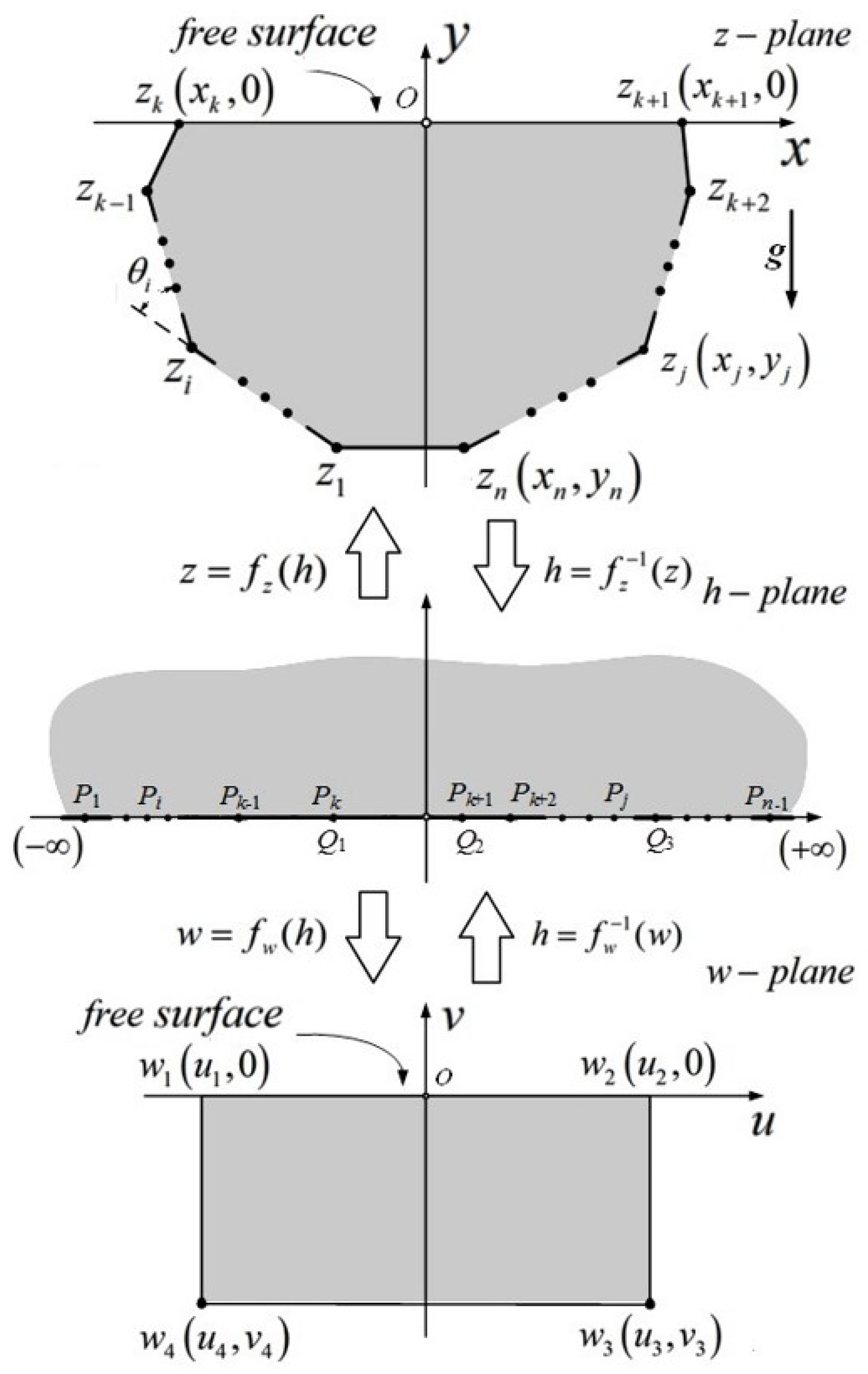
Figure 2.
Coordinate systems.

Figure 3.
Cassini shape tank.
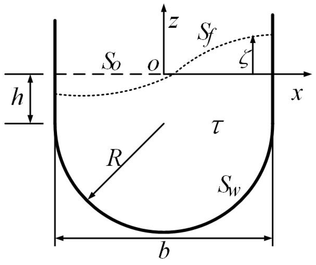
Figure 4.
Comparisons of theoretical and numerical natural frequencies.
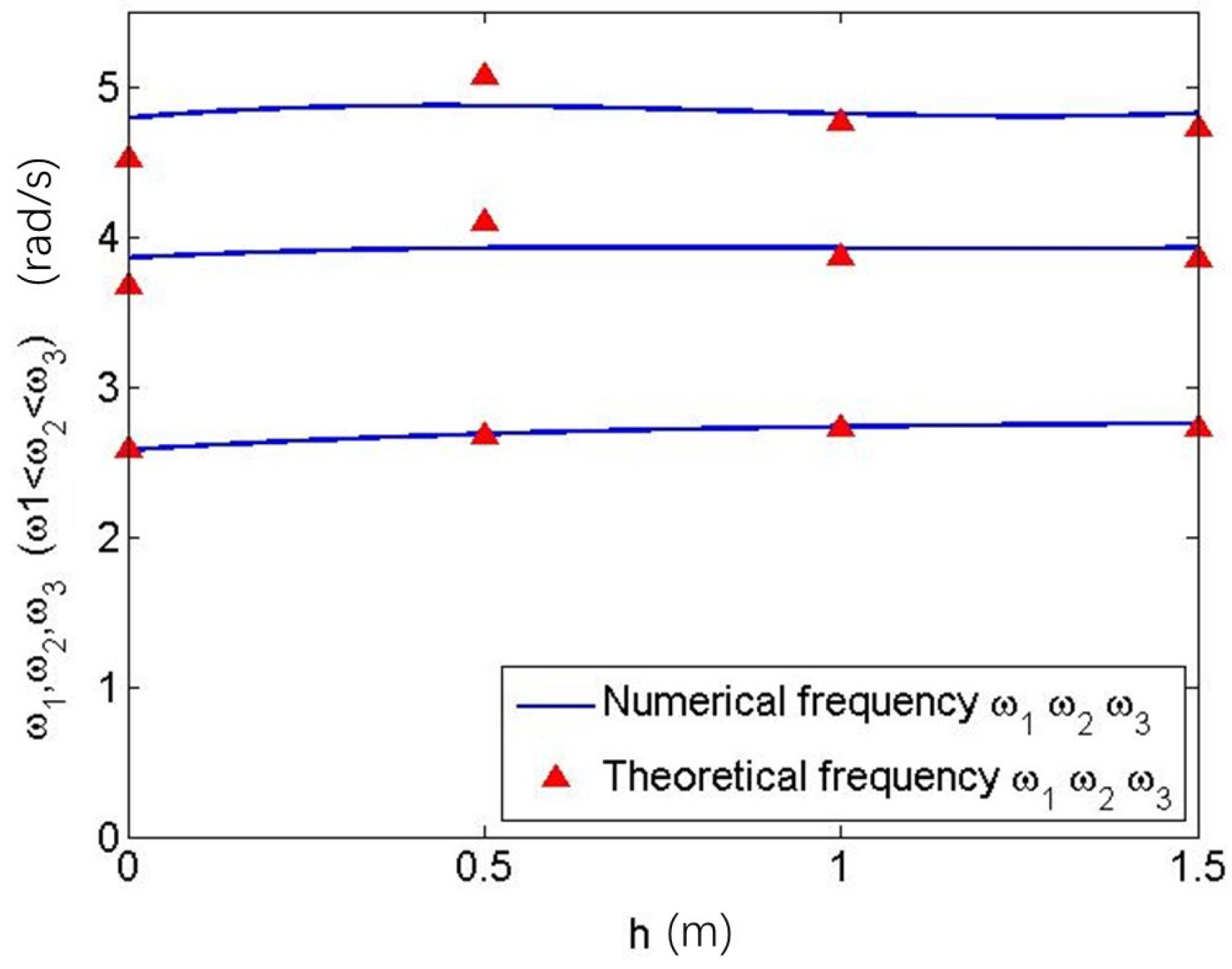
Figure 5.
Slosh forces, moments, and coefficients of wave function at .
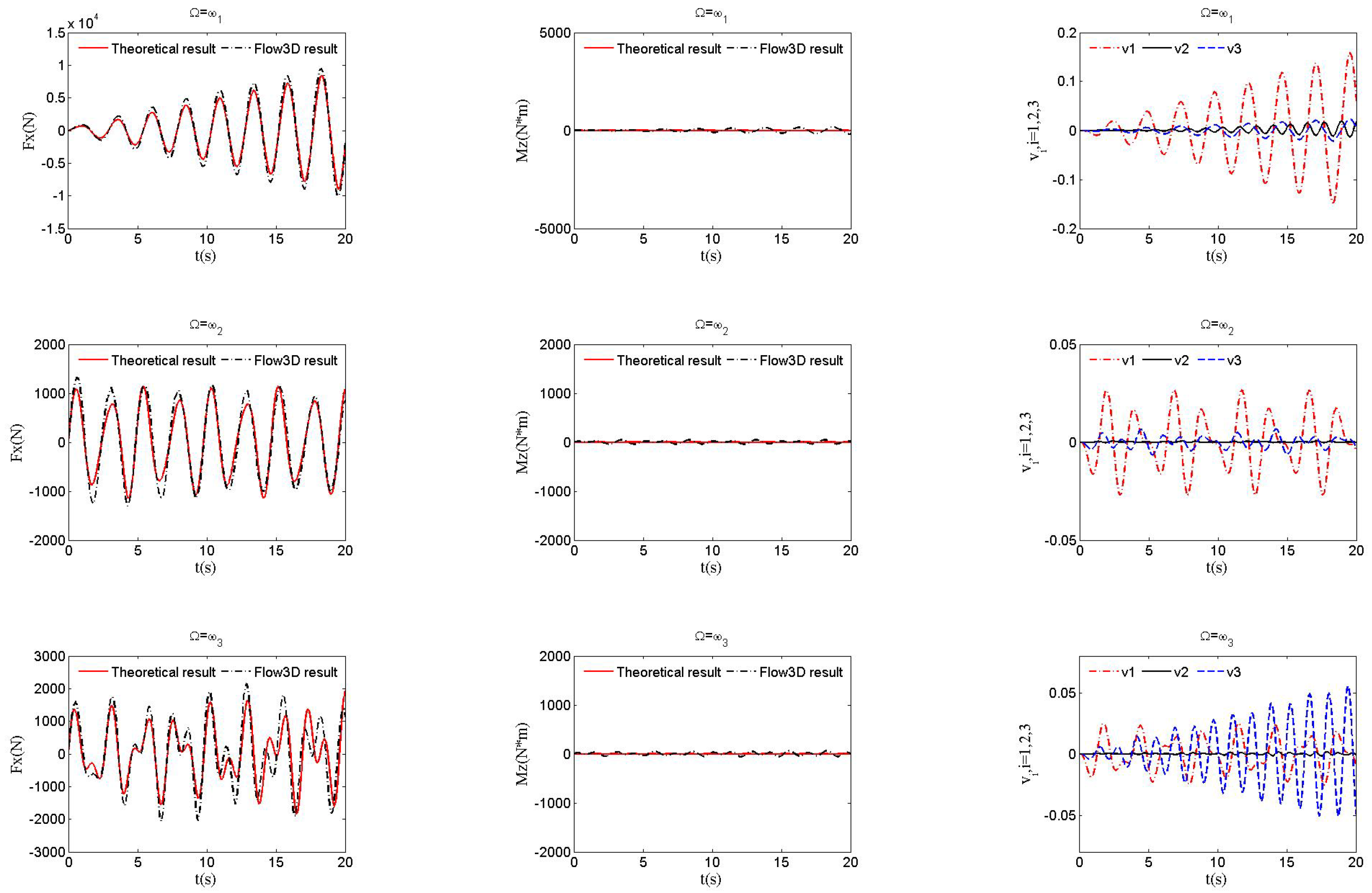
Figure 6.
Slosh forces, moments, and coefficients of wave function at .
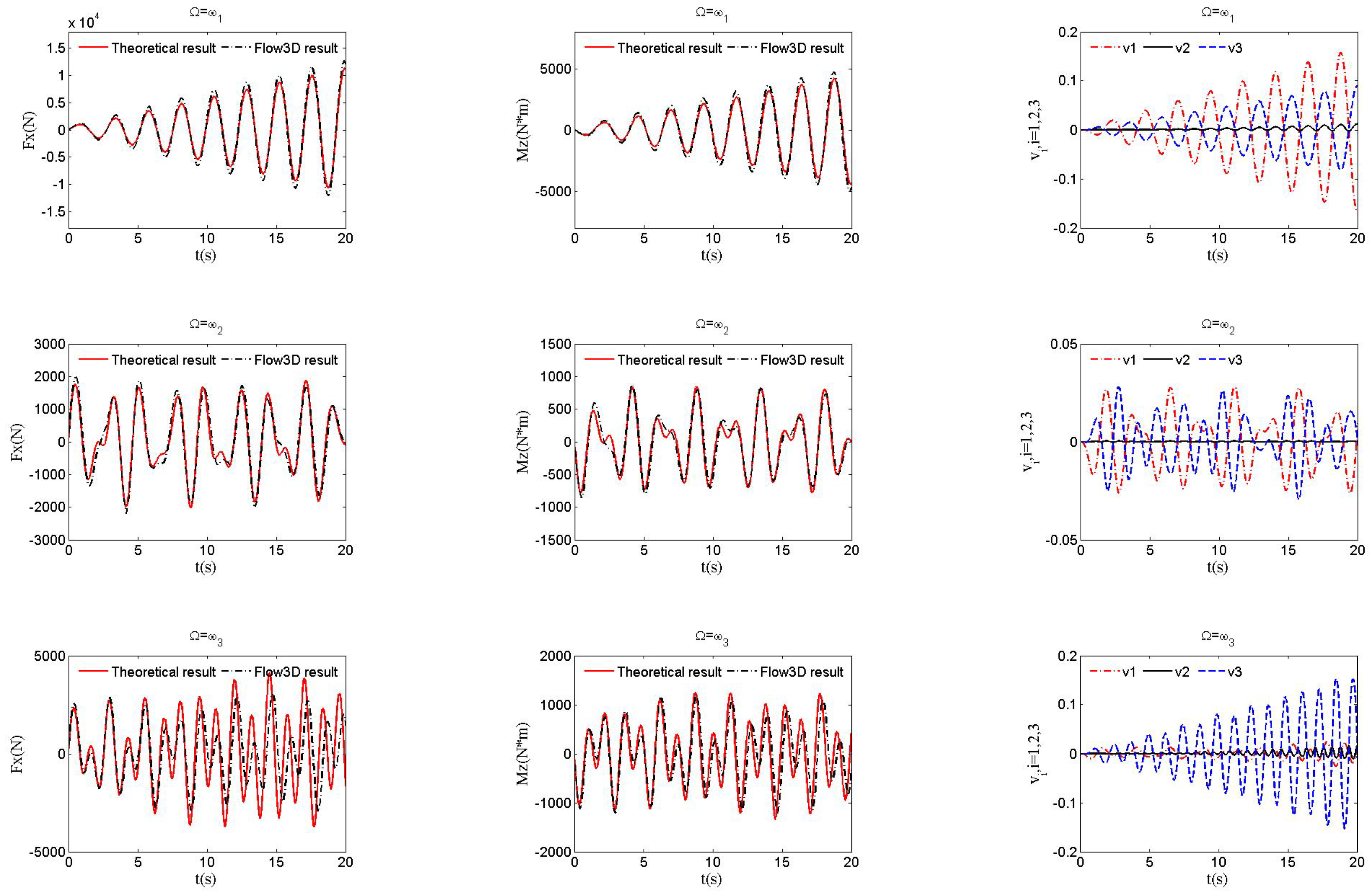
Figure 7.
Slosh forces, moments, and coefficients of wave function at .
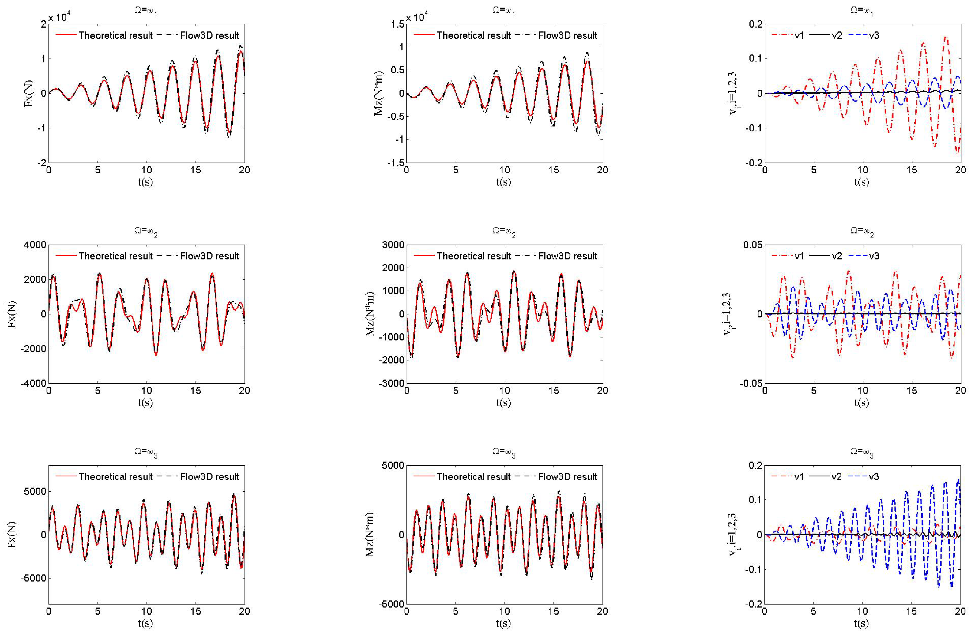
Figure 8.
Slosh forces, moments, and coefficients of wave function at .
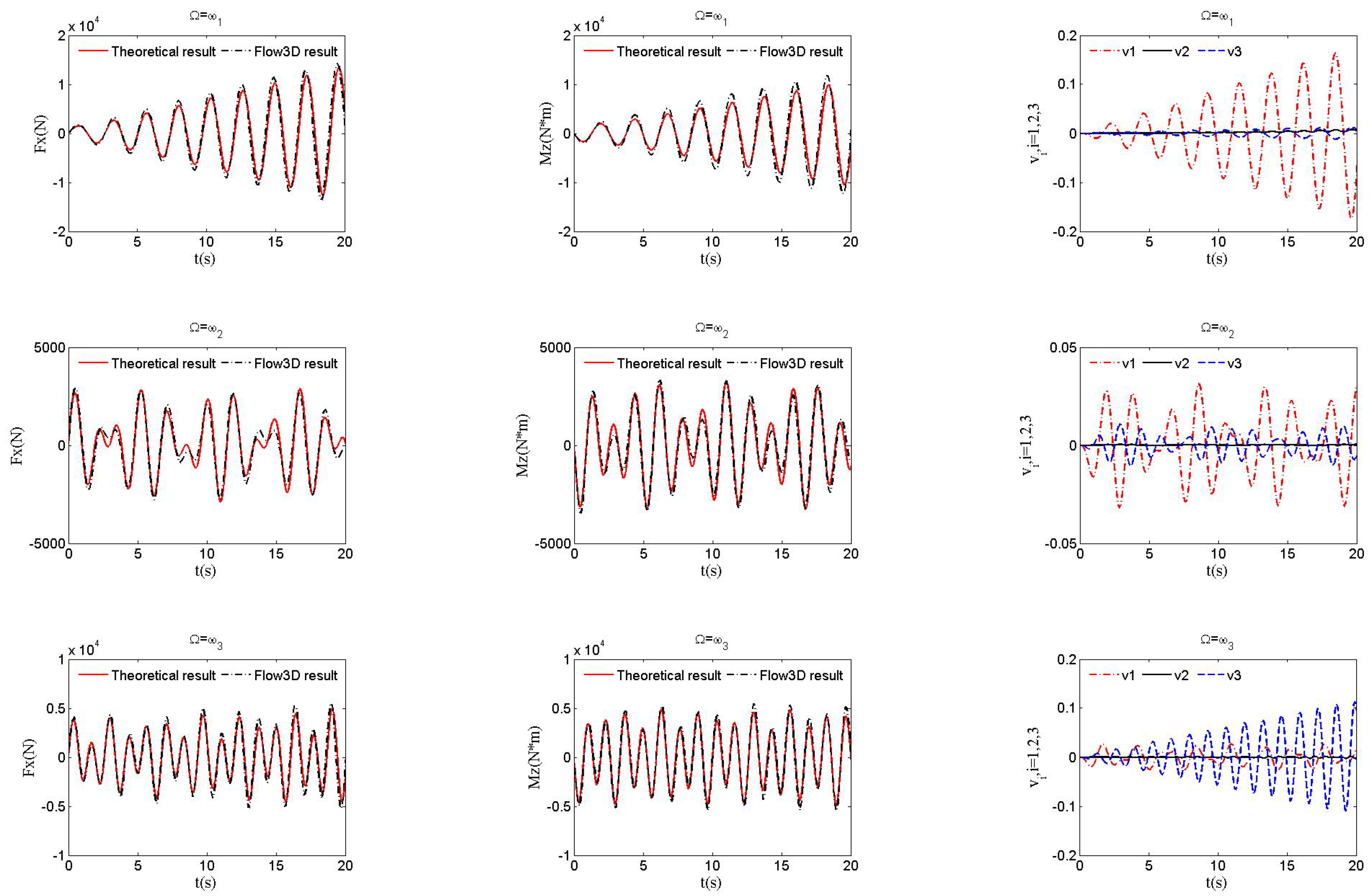
Table 1.
Natural frequencies for different h.
| h (m) | Frequencies for Liquid Sloshing (rad/s) | Frequencies for Coupled System (rad/s) | ||||
|---|---|---|---|---|---|---|
| 1st Order | 2nd Order | 3rd Order | 1st Order | 2nd Order | 3rd Order | |
| 0 | ||||||
| 1 | ||||||
Disclaimer/Publisher’s Note: The statements, opinions and data contained in all publications are solely those of the individual author(s) and contributor(s) and not of MDPI and/or the editor(s). MDPI and/or the editor(s) disclaim responsibility for any injury to people or property resulting from any ideas, methods, instructions or products referred to in the content. |
© 2024 by the authors. Licensee MDPI, Basel, Switzerland. This article is an open access article distributed under the terms and conditions of the Creative Commons Attribution (CC BY) license (https://creativecommons.org/licenses/by/4.0/).
Share and Cite
MDPI and ACS Style
Lü, J.; Zhu, X.; Yu, Y. A Two-Dimensional Liquid Sloshing Analysis in a Partially Filled Complicated-Shape Tank by the Schwarz–Christoffel Transformation. Acoustics 2024, 6, 346-361. https://doi.org/10.3390/acoustics6020018
AMA Style
Lü J, Zhu X, Yu Y. A Two-Dimensional Liquid Sloshing Analysis in a Partially Filled Complicated-Shape Tank by the Schwarz–Christoffel Transformation. Acoustics. 2024; 6(2):346-361. https://doi.org/10.3390/acoustics6020018
Chicago/Turabian StyleLü, Jing, Xiaolong Zhu, and Yang Yu. 2024. "A Two-Dimensional Liquid Sloshing Analysis in a Partially Filled Complicated-Shape Tank by the Schwarz–Christoffel Transformation" Acoustics 6, no. 2: 346-361. https://doi.org/10.3390/acoustics6020018