Tunnel Effect for Ultrasonic Waves in Tapered Waveguides

Abstract

Traversal time in the tunneling effect for ultrasonic waves in tapered waveguides is derived considering its analogy with quantum and electromagnetic wave tunneling. If, as traversal time, the so-called phase time is considered, the ultrasonic wave packet shows the equivalent in acoustics of superluminality, i.e., the derived velocity, crosses the limit of bulk transverse ultrasonic waves in the medium of the waveguide that is the equivalent of c in the quantum and electromagnetic cases. The graphs clearly illustrating this so-called Hartman effect are obtained confirming the experimental results in the three different fields.

1. Introduction

The existence of a formal analogy among the equations that govern wave propagation allows for the extension of, in some cases, the results of the phenomena whose study originates in areas of different physical disciplines. This is the case, for example, of the phenomenon of the so-called superluminal propagation of evanescent waves, whose name directly recalls the field of electromagnetism, but which also has close analogies in quantum physics and, as demonstrated in this paragraph, even in acoustics. The unifying concept is that of the propagation of an impulse or a wave packet in a medium with a strong or anomalous dispersion: a packet of acoustic, electromagnetic or quantum wave probability density waves can therefore be considered equivalent.

Let us therefore imagine not a monochromatic wave but a wave packet limited in time and space with a central carrier frequency and an envelope with a modulated amplitude, which, therefore, introduces components at different frequencies through the Fourier analysis: the so-called phase velocity $V_f=\omega /k$ can be identified as the velocity of the crests of the carrier frequency, but already Lord Rayleigh [1] identified the fact that the packet envelope moves with the group velocity $V_g=d\omega /dk$ (at first order), which has, in the case of anomalous dispersion, peculiar characteristics, e.g., can become negative when the frequency decreases rather than increases with increasing k.

Anomalous dispersion was first studied for mechanical oscillators [2] and later, by Sommerfeld and Brillouin, in materials that absorb light in which the group velocity can be greater than c (the velocity of light in vacuum) or even negative within the absorption [3]. The phase velocity can be greater than c in many cases, for example, inside waveguides, but this does not create problems because, representing the velocity of a continuous series of crests, this does not carry the signal information.

On the other end, if the group velocity is identified as the velocity at which a signal (information) travels, the problem of the limit of the principle of causality set by the constancy of the velocity of light in the vacuum of special relativity immediately arises, but this identification is possible only in cases of “normal” dispersion where the deformation of the packet is slight and the group velocity remains below the velocity c.

Sommerfeld and Brillouin then continued to define signal velocity as that of the point of rise of the signal intensity equal to half its steady-state value, which can be demonstrated to proceed at the group velocity, but they introduced the concept of “velocity of the wave front” ideally defined as that of a discontinuity in the signal of the step function type with an infinite derivative and it is this last velocity, certainly carrying information, which is subject to the limitation of the velocity c just as the velocity, to be defined, with which the energy is transported [3,4].

All these velocities, in a non-dispersive medium coincide and are equivalent, for elastic waves, to the bulk transverse waves velocity of that medium while, for electromagnetic waves, it is the velocity of light in that medium or c if it is a vacuum. However, it must be noted that the definition of a wave front with an infinite derivative (vertical slope) is only ideal, requiring an infinite bandwidth in the frequency components, which is unachievable in any real signal generator. In reality, physical signal generators only produce a finite spectra due to their natural inertia in reaching the steady-state amplitude (impossibility of a vertical rise of the wave front) and the necessarily finite content of energy in the signal because an infinite frequency bandwidth would require, due to the Plank relation $E=\hslash \omega$, an infinite energy.

The limitation of the frequency bandwidth for a physical detector highlights the limits of reasoning based on classical physics. In the latter case, a “classical” detector can detect a theoretically small quantity of energy as desired, whereas a physical detector needs at least a quantum of energy $\hslash \omega$. Regardless of the interpretation, when we talk about propagation at superluminal velocity, we are referring to a clear and measurable effect that involves the group velocity and therefore requires the use of a wave packet. This effect has been predicted theoretically and measured experimentally in different conditions: for example, in anomalous dispersion zones near an absorption line [5,6,7], in nonlinear [8] and linear gain lines [9,10,11], in a active plasma [12], optically [13] and, finally, in a tunnel effect barrier [14,15,16,17].

This last physical situation in which superluminal wave packets are found, is the one we want to take into consideration here because there is a close analogy between the quantum tunneling effect of a particle through a potential barrier and the crossing of a zone, limited in space, in which propagation is prohibited for both electromagnetic- and acoustic-guided wave packets.

The so-called Hartman effect [18] has been theoretically analyzed [19] and experimentally measured in different fields [16,20,21] for which the crossing time of a quantum potential barrier [22] initially increases with the dimensions of the barrier and then rapidly reaches a constant value, which is of the order of magnitude of the inverse of the carrier frequency of the wave packet, independent of the dimensions of the barrier. It is immediate that, by simply defining the velocity of crossing the barrier as the ratio between its dimensions and the time taken to cross it, the velocity grows with the dimensions of the barrier when the time reaches a constant value, until it reaches superluminal values.

It is necessary to point out, however, in this phenomenon that the time considered is that of detecting the half height of the rise of the wave front, therefore, we are talking about the observation of the packet envelope, which should correspond to the group velocity, on the other hand, the superluminal velocity defined in this way is not a real velocity that can be defined at every point, since, inside the barrier where the waves are evanescent, there is no defined propagation and corresponding velocity. Other possible definitions of the tunneling crossing time and the corresponding velocity are possible, although the interpretations are not unambiguous [23,24].

Having this said, let us focus on the fact that the tunneling phenomenon is essentially a wave one. So the same principles and the same equations, in opportune cases, can be applied for very different kinds of waves, from the quantum wave functions to the electromagnetic waves to, and this is the case of interest here, the acoustic or ultrasonic waves in matter. The key point is that there must exist a zone where the propagation is forbidden and the waves become evanescent; the limitation in extension of this zone permits the propagating wave to resume after the end of the “barrier”, even with a different amplitude and phase with respect to the normal propagation but in a way that it is possible to imagine that the wave will succeed to cross the barrier in a certain time and with a certain speed.

The importance of the ultrasonic simulation of phenomena, originally studied in other fields, thanks to the analogy of the equations, in specific cases, has been increasingly pointed out in recent years. From the analogy of the acoustic black hole with the optical one [25], to the quantum phenomenon of Hawking radiation [26], a simulation with ultrasound adds the possibility to study a phenomenon in conditions impossible to have in the original situation and with a rescaling and changing of the measurable quantities that amplifies the studying of details non-reachable otherwise.

So, in our case, it is possible to reply and rescale the measurable quantities like traversal time and signal intensity and frequency in a way that is more accessible than in the quantum and electromagnetic fields. Moreover, further details can be studied like, for example, the field inside the barrier being almost impossible to examine in other situations. In this article, the conjecture about the traversal time of an “opaque” barrier being of the same order of the inverse of the used frequency and the demonstration of its independence via the opaque barrier length have been found for ultrasonic-guided waves. The rescaling and the specifics of the ultrasonic-guided waves’ environment opens the way to experiments that promise more detailed results than the ones possible in the other mentioned fields.

2. Material and Methods

2.1. Analogy between the Quantum Tunneling Effect and Evanescent, Electromagnetic- or Acoustic-Guided Waves

Recall that the Schrödinger equation leads to a negative kinetic energy in the case of tunneling since the potential energy V is greater than the total energy of the particle E; the equation for a one-dimensional barrier is

$$\frac{d^2\psi }{d{x}^2}+2\frac{m}{{\hslash }^2}(E-V)\psi =0.$$

(1)

where m the mass of the particle, E its total energy and V the potential energy of the barrier.

• Its monochromatic solution leads to evanescent modes within the barrier (where V > E) of the type

  $${\psi }_{(V>E)}=A{e}^{-qx}+B{e}^{+qx}$$

  (2)

  where q is such that, having defined the free de Broglie wavenumber as $k=\sqrt{2mE/{\hslash }^2}$, which becomes $k^{\prime }=\sqrt{2m(E-V)/{\hslash }^2}$ if a potential $V<E$ is present, is defined as $q=-𝚤k^{\prime }=\sqrt{2m(V-E)/{\hslash }^2}$ inside the barrier where $V>E$.

So, defining for the barrier a characteristic $k_0=\sqrt{k^2+q^2}=\sqrt{2mV/{\hslash }^2}$, then it is possible to write down the Schrödinger equation as

$$\frac{d^2\psi }{d{x}^2}+(k^2-k_0^2)\psi =0.$$

(3)

The Schrödinger equation is then completely analogous to the Helmholtz equation for guided waves. This equation is applicable to both guided electromagnetic waves and guided acoustic waves, where $\psi$ represents the electric field inside the waveguide in the former case and the polarized displacement in the horizontal transverse direction, relative to the typical waveguide axis, of the so-called SH (Shear Horizontal) in the latter case of acoustic-guided waves.

For guided waves, k is then the wavenumber of the bulk waves of the fields in the material medium considered, while $k_0$ is the cut-off wavenumber of the guide such that $k_0=n\pi /b$, where $n=1,2,3\dots$ is the order of the possible propagation modes inside a guide of thickness b.

In a wave guide, it is therefore possible to simulate a potential barrier by narrowing the guide along section d in such a way that $k_0>k$ and, therefore, the propagation wave number in the direction of the guide axis $\beta =\sqrt{k^2-k_0^2}$ becomes imaginary, giving rise to evanescent waves inside the narrowed part of the guide. For the electromagnetic waves $k=\omega /v$, where v is the bulk velocity of the wave in the material while for the ultrasonic SH waves $k=\omega /V_s$ with $V_s$ the velocity of the transverse bulk waves in the medium considered.

The quantum tunneling effect happens when the particle, represented by a wave packet of the probability density wave function with central frequency corresponding to the De Broglie wavelength, passes through an area in which a forbidden potential barrier is present, therefore, it has a precise analogy with the propagation of a packet of electromagnetic or acoustic waves within a tapered guide in such a way that the waves are evanescent in the narrowed, limited area representing the barrier.

The equations describing the quantum tunneling effect can be transformed in the ones describing the propagation, in a waveguide, through a forbidden barrier with the substitution

$$\frac{\hslash }{m}⟶\frac{v^2}{\omega }$$

(4)

where v is the bulk electromagnetic wave velocity or the bulk ultrasonic wave transverse velocity in the material that constitutes the waveguide.

2.2. A Possible Definition of Traversal Time: The Phase Time

Let us consider the solution of a one-dimensional Schrödinger equation for a given value of energy E in presence of potential barrier V. The solution can be expressed in three parts, ${\psi }_1\left(x\right)$, ${\psi }_2\left(x\right)$ and ${\psi }_3\left(x\right)$, respectively, the wave function, on the left, inside and on the right of the barrier, as in Figure 1:

$$\begin{array}{ccc}\hfill {\psi }_1\left(x\right)& =& A{e}^{+𝚤kx}+B{e}^{-𝚤kx}\hfill \\ \hfill {\psi }_2\left(x\right)& =& C{e}^{-qx}+D{e}^{+qx}\hfill \\ \hfill {\psi }_3\left(x\right)& =& F{e}^{+𝚤kx}.\hfill \end{array}$$

(5)

Considering a rectangular-shaped potential barrier placed along the x axes between positions $x=0$ and $x=d$, the boundary conditions of continuity of the wave function and of its derivative lead to a system for the wave amplitudes to solve:

$$\begin{array}{ccc}\hfill A+B& =& C+D\hfill \\ \hfill 𝚤k(A-B)& =& -q(C-D)\hfill \\ \hfill C{e}^{-qd}+D{e}^{+qd}& =& F{e}^{𝚤kd}\hfill \\ \hfill -q(C{e}^{-qd}-D{e}^{+qd})& =& 𝚤kF{e}^{𝚤kd}.\hfill \end{array}$$

(6)

Eliminating the amplitudes B, C and D, it is possible to find the complex transmission coefficient $\sqrt{T}{e}^{𝚤\alpha }$ such that

$$\sqrt{T}{e}^{𝚤\alpha }\equiv \frac{F}{A}=\frac{4𝚤kq}{-{(q-𝚤k)}^2{e}^{qd}+{(q+𝚤k)}^2{e}^{-qd}}{e}^{-𝚤kd},$$

(7)

and an analogous expression for the reflection coefficient $R=B/A$.

It is given a wave packet strictly picked around value k, impinging on the barrier; its Fourier components will be of the form $\sqrt{T\left(k\right)}$exp$[𝚤\alpha (k)+𝚤kx-𝚤E(k)t/\hslash ]$. The transmitted wave packet will be thus described by the expression

$${\psi }_T=\frac{1}{\sqrt{2\pi }}{\int }_{-\infty }^{+\infty }\sqrt{T\left(k\right)}{e}^{𝚤\alpha \left(k\right)}{e}^{kx}{e}^{-𝚤\omega \left(k\right)t}dk$$

(8)

where, for a particle, $\omega \left(k\right)=E\left(k\right)/\hslash$.

The phase time is the time associated with a recognizable element of the packet such as, for example, the peak to which we assign a position $x\left(t\right)$. To follow the peak, we can use the stationary phase method: we rewrite the exponential in the integral as $e^{𝚤F\left(k\right)}$, where $F\left(k\right)$ represents the total changing of phase of the individual components, with a phase shift due to propagation with the path inside the barrier, included. The method, therefore, consists of neglecting the contribution to the integral in the regions in which $F\left(k\right)$ varies rapidly with k, since the rapid oscillations of the function tend to give a null contribution to the integral. The main contribution to the integral comes instead from the regions around the extremal points of $F\left(k\right)$, those where the first derivative with respect to k vanishes [14]. This leads to the equation

$$\frac{d\alpha }{dk}+x\left(t\right)-\frac{d\omega }{dk}t=0;$$

(9)

thus the process of tunneling through a barrier of length d leads to a spatial delay $\delta x=d\alpha /dk$ and the traversal phase time $t_T^{\varphi }$ is defined as the ratio of the spatial delay due to the overall phase shift to the group velocity $v_g$ [27].

From Equation (7)

$$\frac{F}{A}{e}^{𝚤kd}=T^{1/2}{e}^{𝚤\left(\alpha \right(k)+kd)}=\frac{2kq}{2kqcosh\left(qd\right)-𝚤(k^2-q^2)sinh\left(qd\right)}$$

(10)

so the phase displacement

$$\alpha \left(k\right)+kd={tan}^{-1}\left[\frac{k^2-q^2}{2kq}tanh\left(qd\right)\right].$$

(11)

The phase time for the barrier crossing is then

$$t_T^{\varphi }=\frac{1}{v_g}\frac{d}{dk}(\alpha \left(k\right)+kd)=\frac{m}{\hslash kq}\frac{2qd{k}^2(q^2-k^2)+k_0^{4}sinh\left(2qd\right)}{4k^2{q}^2+k_0^{4}sinh\left(qd\right)}$$

(12)

The time defined in this way is certainly an important reference concept, but it is necessary to mention why this definition does not conclude the theoretical discussion, indeed other definitions of traversal time have been hypothesized and the problem is still open.

Problems with Phase Time

Let us consider the reflection phase time $t_R^{\varphi }$ (defined in the same way as $t_T^{\varphi }$ but now for the reflected particle) and the dwell time $t_D^{\varphi }$ (dwell time) [28] defined as the average time spent by the particle in a certain spatial interval $(x_1,x_2)$, which may possibly include the expression barrier having the expression

$$t_D^{\varphi }=\frac{1}{J\left(k\right)}{\int }_{x_1}^{x_2}{\left|\psi (x,k)\right|}^{2}dx$$

(13)

that is the ratio between the number of the particles in the interval that includes the barrier and the flux of the incident probability density $J\left(k\right)=\hslash k/m$.

Then, necessarily, the condition $t_D^{\varphi }=R{t}_R^{\varphi }+T{t}_T^{\varphi }$ where R and T are, respectively, the reflexion and transmission coefficients, should be satisfied. In our case, instead, there is an additional sinusoidal term [14,23,29]:

$$t_D^{\varphi }=R{t}_R^{\varphi }+T{t}_T^{\varphi }+\frac{\sqrt{R}}{k{v}_g}sin(\mathrm{\Phi }-2k{x}_1)$$

(14)

where $\mathrm{\Phi }$ is the phase displacement of the reflected wave. This term represents the interference between the reflected wave function and the one incident on the barrier. Since, to define the velocity of crossing the barrier, we need the actual traversal time taken by the particle (or by the wave packet) to cross it, the phase transmission time $t_T^{\varphi }$, as defined above, cannot represent the actual traversal time because it contains an additional interference term in which the contributions of transmission and reflection are not separable.

2.3. $SH$ Modes in Ultrasonic Waveguides

It is given an ultrasonic rectangular waveguide, characterized by an ideally infinite length (direction z) along which the waves propagate, an ideally infinite width (direction y) and a finite thickness b (direction x) comparable with the wavelength. The normal stress-free condition at the surface of the waveguide rules the propagation of the possible modes. With respect to the waveguide, it is possible to distinguish three polarizations of the ultrasonic waves. The longitudinal one L and, of the two shear, the one polarized in the vertical direction ($SV$) along the thickness and the other polarized in the horizontal direction ($SH$) along the width of the waveguide.

When a shear horizontal wave is reflected at the interface constituted by the waveguide surfaces, the boundary conditions are fully satisfied by a reflection in another $SH$ wave, while the shear vertical $SV$ is partially reflected and partially transformed in a longitudinal L and so the longitudinal generates at reflection both the $SV$ and L kind. So two kinds of modes can propagate along the waveguide, the pure shear modes, horizontally polarized, $SH$ and modes that are a combination of longitudinal ad shear vertical polarization called Lamb modes.

Let us focus on the $SH$ modes that have a dispersion relation that is the analogue of the electromagnetic and quantum cases and has an analytic expression for the function $\omega \left(k\right)$ while the dispersion relation for Lamb waves must be solved numerically to obtain the function $\omega \left(k\right)$. From a mathematical point of view, it is possible to define a displacement vector $\overrightarrow{u}$, a scalar potential $\varphi$ and a vector potential $\overrightarrow{\psi }$ such that

$$\overrightarrow{u}=\nabla \varphi +\nabla \times \overrightarrow{\psi }.$$

(15)

Through Christoffel equation for isotropic medium [30], it is possible to demonstrate that the shear waves depend only on $\overrightarrow{\psi }$ with a wave equation

$$\mathsf{\Delta }\overrightarrow{\psi }-\frac{1}{v_s^2}\frac{{\partial }^2\overrightarrow{\psi }}{\partial t^2}=0$$

(16)

where $v_s$ is the shear bulk velocity $v_s=\sqrt{\mu /\rho }$ and $\mu$ is the shear modulus [31].

In the rectangular waveguide, the $SH$ waves reflect on themselves back and forth between the surfaces. Their shear wavenumber vector of modulus $k_s=\omega /v_s$, has transversal component $k_{ts}$ along y direction and component $\beta$ along the direction of propagation z. $SH$ waves have the only displacement component along the horizontal direction x, so the vector potential $\overrightarrow{\psi }$ has the only component along the vertical y direction such that

$${\psi }_y=A{e}^{-𝚤\beta z}cos(k_{ts}y+\alpha )$$

(17)

and

$$u_x=-\frac{\partial \psi }{\partial z}=𝚤\beta {\psi }_y=𝚤\beta A{e}^{-𝚤\beta z}cos(k_{ts}y+\alpha ).$$

(18)

The boundary conditions impose the component of the stress, normal to the surfaces

$$T_{xy}=\mu \frac{\partial u_x}{\partial y}=𝚤\beta k_{ts}\mu A{e}^{-𝚤\beta z}sin(k_{ts}y+\alpha ),$$

(19)

to be null at $y=\pm b/2$. This leads to $\alpha =0$ and to the condition of transverse resonance given by

$$k_{ts}=\frac{n\pi }{b}(n\in \mathbb{N}).$$

(20)

So a number n of $SH$ modes exist that satisfy the boundary conditions and that have a wavenumber of propagation $\beta$ such that

$${\beta }^2=k_{ts}^2-{\left(\frac{n\pi }{b}\right)}^2={\left(\frac{\omega }{v_s}\right)}^2-{\left(\frac{n\pi }{b}\right)}^2.$$

(21)

This dispersion relation is the analogue of that of the electromagnetic waveguide. Excluding the $n=0$ mode, which is simply a shear bulk wave propagating parallel to the z direction, all the other modes have a cut-off frequency below which the mode is evanescent.

2.4. Phase Time for $SH$ Ultrasonic Waves

The transmission phase time $t_T^{\varphi }$, as defined in Section 2.2, is an important reference concept that can also be defined in the acoustic field. Let us consider its expression for a potential barrier simulated by a zone in which the waves become evanescent (e.g., an area with less thickness than a waveguide such that the frequency is under the cut-off limit) for $SH$ waves. A waveguide of thickness b is considered in which the propagation of a particular $SH$ mode is possible with dispersion Equation (21)

$$\beta =\sqrt{\frac{{\omega }^2}{v_s^2}-{\left(\frac{n\pi }{b}\right)}^2}$$

(22)

where the wave vector $\overrightarrow{\beta }$, of the propagating wave along the waveguide, is real and the propagating mode has expression

$$\psi ={\psi }_0{e}^{𝚤(\beta z-\omega t)}$$

(23)

In the narrowed section of the waveguide of length d, if the thickness $b^{\prime }$ is such that $b^{\prime }<n\pi v_s/\omega$, the correspondent ${\beta }^{\prime }$ becomes imaginary and it is substituted by

$$q=𝚤{\beta }^{\prime }=\sqrt{{\left(\frac{n\pi }{b^{\prime }}\right)}^2-\frac{{\omega }^2}{v_s^2}}$$

(24)

and the wave becomes evanescent with expression

$$\psi ={\psi }_0{e}^{-qz}{e}^{𝚤\omega t}.$$

(25)

Defining, then

$$k_0=\sqrt{{\left(\frac{n\pi }{b^{\prime }}\right)}^2-{\left(\frac{n\pi }{b}\right)}^2},$$

(26)

the traversal phase time for $SH$ waves has an expression analogous to (12)

$$t_T^{\varphi }=\frac{1}{v_{g}q}\frac{2qd{\beta }^2(q^2-{\beta }^2)+k_0^{4}sinh\left(2qd\right)}{4{\beta }^2{q}^2+k_0^{4}sinh\left(qd\right)}$$

(27)

where the group velocity is $v_g=v_s^2\beta /\omega$.

3. Results

3.1. Theoretical Results for SH Waves

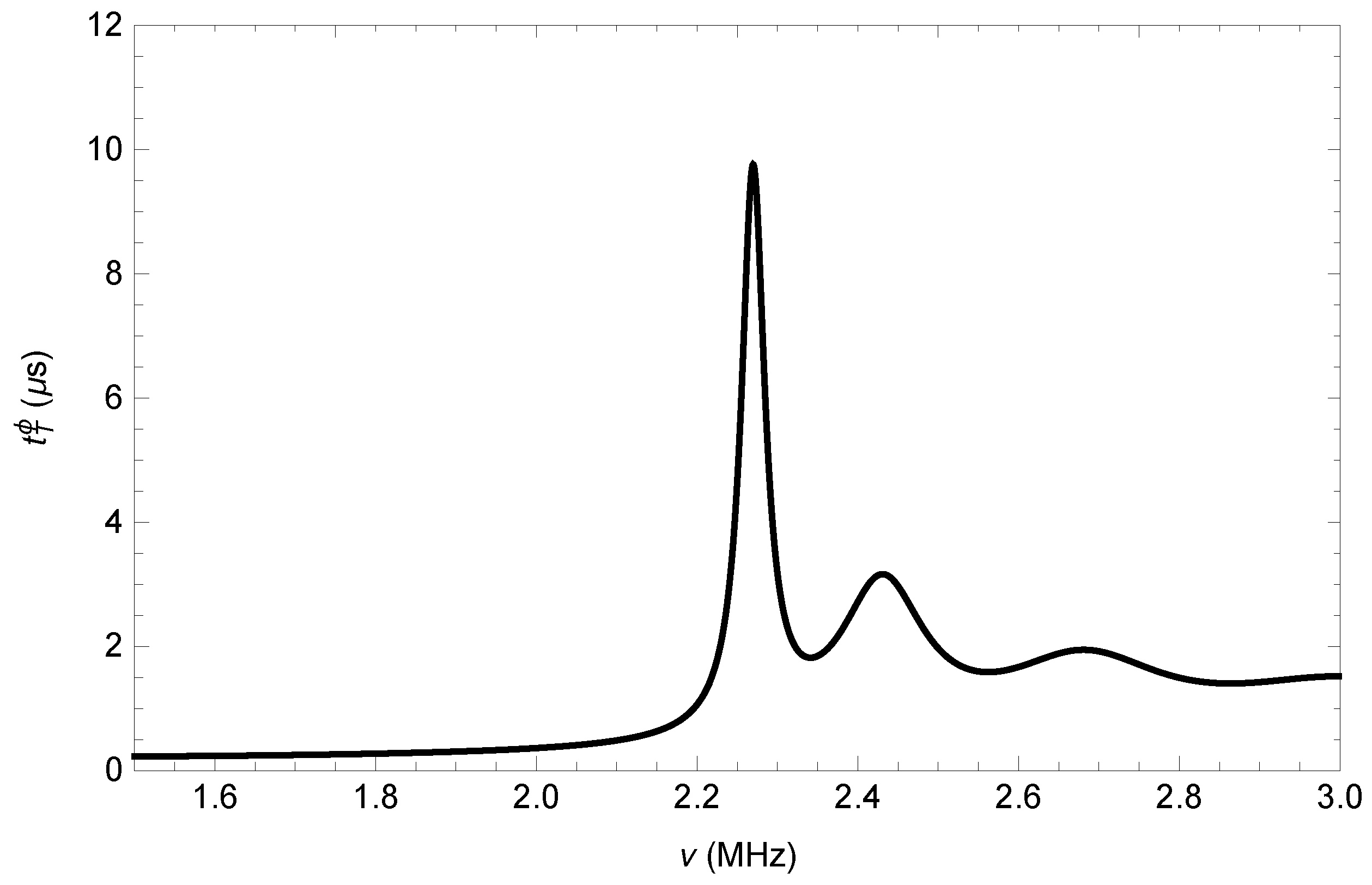
In a concrete example, we can consider a waveguide with the thickness $b=2$ mm tapered in an area with a smaller thickness of $b^{\prime }=0.7$ mm, of length d; the velocity of the transverse waves is set to $v_s=3100$ m/s, which is typical of aluminum. In this case, it is found that the cut-off frequency of the evanescent wave zone is ${\nu }_0=2.214$ MHz. In Figure 2, the phase time is graphed as a function of frequency for the first mode $n=1$ and a barrier $d=3$ mm long. To be noted, the barrier resonances above the cut-off frequency and the monotonic decrease in traversal time below the cut-off frequency.

If we adjust the width frequency $\nu =2.200$ MHz (wavelength $\lambda =1.41$ mm) just below the cut-off frequency ${\nu }_0=2.214$ MHz, in

Table 1. Traversal phase time and velocity for different lengths of the barrier for $SH$ waves at frequency $\nu =2.200$ MHaz and cut-off frequency ${\nu }_0=2.214$ MHz.

Barrier Length d (mm)	Traversal Phase Time ${\mathit{t}}_{\mathit{T}}^{\mathit{\varphi }}$ ($\mathbf{\mu }$s)	Traversal Velocity ${\mathit{V}}_{\mathit{T}}$ (m/s)
3	1.0646	2818.0
8	1.3489	5930.6
13	1.3543	9598.9
18	1.3544	13,290.2
23	1.3544	16,981.9
28	1.3544	20,673.7

are indicated the values of the traversal phase time ${\tau }_T^{\varphi }$ and the corresponding traversal velocity $V_T$ defined as the ratio between the length of the barrier (evanescent zone) and the traversal phase time, corresponding to different lengths d of the barrier. It is possible to note the so-called Hartman effect, for which the traversal time tends to a constant limit value, independent of the barrier length, resulting in a rapid increase in traversal velocity; the effect happens when, increasing the barrier length d, it becomes opaque, i.e., $\beta d\gg 1$. Remembering that the velocity of the bulk transverse waves $v_s=3100$ m/s represents the analogue of the velocity of light in the medium that constitutes the electromagnetic wave guide, it is possible to note that, with these parameters, the acoustic analogue of the apparent superluminal behavior is already reached with a barrier length corresponding to few wavelengths of the signal.

At lower frequencies then, i.e., further inside the potential well, the Hartman effect is reached even for shorter barrier lengths and the value of the traversal time limit decreases slightly and it is within the order of magnitude of a fraction of a microsecond.

This is graphed in Figure 3, where the phase time is in the function of the barrier length for several frequencies under the cut-off. The plateau of constant phase time, showing the Hartman effect, is reached for lower frequencies at shorter barrier lengths.

Defining the traversal velocity as the ratio between barrier length and phase time increment during the crossing; in Figure 4, it is possible to see at which barrier length the value of this velocity goes above the limit velocity of shear bulk waves in the material for different frequencies. The lower the frequency, the shorter the barrier length is necessary to cross above this limit.

3.2. Some Experimental Results in the Literature

The traversal time measurements in the tunneling effect in quantum mechanics pose several problems for issues related to non-invasive measurements of quantum objects [22]. In electromagnetism and acoustics, measurements of the delay of the packet envelope were instead carried out for different frequencies and in different situations in which evanescent waves were involved.

Table 2. Experimental results in the literature.

Barrier Type	Reference	Traversal Time	1/Frequency
FTIR	Balcou and Dutriax [32]	40 fs	11.3 fs
FTIR	Mugnai et al. [33]	134 ps	100 ps
FTIR	Carey et al. [34]	≈1 ps	3 ps
FTIR	Haibel and Nimtz [35]	117 ps	120 ps
Photonic chain	Steinberg et al. [13]	1.47 fs	2.3 fs
Photonic chain	Spielmann et al. [20]	2.7 fs	2.7 fs
Photonic chain	Nimtz et al. [36]	81 ps	115 ps
Photonic waveguide	Enders and Nimtz [37]	81 ps	115 ps
Microwave waveguide	Ranfagni et al. [15]	≈1 ns	≈1 ns
Ultrasonic waveguide	Alippi et al. [38]	0.5 $\mathrm{\mu }$s	0.65 $\mathrm{\mu }$s

lists some experimental results in photonics (tunneling between two FTIR total internal reflection prisms, photonic chain of dielectric layers, tapered waveguide), in guided microwaves and in guided Lamb waves.

Table 2 shows experimental results that support a hypothesis made by Nimtz and Stahlhofen [39], for which the traversal time is of the order of magnitude of the reciprocal of the frequency used. This is found for both the electromagnetic waves and acoustic waves. This fact, combined with the Hartman effect of independence of the traversal time from the length of the barrier for “opaque” barriers (beyond a minimum length) leads to the possibility of an envelope of the wave packet traveling at very large velocities, even superluminal for electromagnetic waves and beyond the maximum elastic velocity of the considered medium for elastic waves.

We remember that in any case in particular conditions, the velocity of the envelope does not correspond to the velocity of information transfer, therefore, the causality principle of special relativity remains intact.

4. Conclusions

Following the formal analogy among quantum, electromagnetic and acoustic waves, the problem of the determination of the traversal time of a potential barrier by evanescent acoustic waves has been addressed. The analogy has been demonstrated for the $SH$ (shear horizontal) modes in a rectangular waveguide that have the same analytical form of dispersion relation as quantum and electromagnetic waves; then, with an appropriate tapering of the waveguide, a potential barrier can be simulated. The article focused in particular on the determination of the so-called phase time, i.e., the temporal delay due to a phase displacement for a wave packet crossing a region of forbidden propagation, putting in evidence the so-called Hartman effect also for acoustic modes.

The Hartman effect happens for opaque barriers when the length d is such that $\beta d\gg 1$. The typical traversal time, in that case, is found for $SH$ waves and compared with other results in the literature obtained in different fields, confirming the conjecture that the traversal phase time is proportional to the inverse of the typical frequency of the phenomenon independently from the length of the opaque barrier.

This leads to an increasing in the traversal velocity defined as the barrier length divided by the phase time, well-above the velocity limit relative to the phenomenon in object, which, for acoustic shear-guided waves, is the shear velocity of bulk waves in the material of which the waveguide is made and that is the analogue of the light c velocity in electromagnetic and quantum fields. This simulation of the tunneling effect with ultrasonic-guided waves confirms the results obtained in other fields and opens the possibility to experimental research on other features, like the study of the signal inside the barrier, which is impossible or very difficult to obtain in other fields of physics.

References

- Rayleigh, L. On the Velocity of Light. Nature 1881, XXIV, 382. [Google Scholar] [CrossRef]
- Rayleigh, L. On the theory of anomalous dispersion. Philos. Mag. 1899, XLVIII, 151. [Google Scholar] [CrossRef]
- Brillouin, L. Wave Propagation and Group Velocity; Academic Press: New York, NY, USA, 1960. [Google Scholar]
- Winful, H.G. Group delay, stored energy, and the tunnelling of evanescent electromagnetic waves. Phys. Rev. E 2003, 68, 016615. [Google Scholar] [CrossRef] [PubMed]
- Garrett, C.G.B.; McCumber, D.E. Propagation of a Gaussian light pulse through an anomalous dispersion medium. Phys. Rev. A 1970, 1, 305. [Google Scholar] [CrossRef]
- Chu, S.; Wong, S. Linear pulse propagation in an absorbing medium. Pys. Rev. Lett. 1982, 48, 738. [Google Scholar] [CrossRef]
- Akulshin, A.M.; Barreiro, S.; Lezama, A. Steep Anomalous Dispersion in Coherently Prepared Rb Vapor. Phys. Rev. Lett. 1999, 83, 4277. [Google Scholar] [CrossRef]
- Basov, N.G.; Ambartsumyan, R.V.; Zuev, V.S.; Kryukov, P.G.; Letokhov, V.S. Nonlinear amplification of light pulses. Sov. Phys. JETP 1966, 23, 16. [Google Scholar]
- Chiao, R.Y. Superluminal (but causal) propagation of wave packets in transparent media with inverted atomic populations. Phys. Rev. A 1993, 48, R34. [Google Scholar] [CrossRef]
- Steinberg, A.M.; Chiao, R.Y. Dispersionless, highly superluminal propagation in a medium with a gain doublet. Phys. Rev. A 1994, 49, 2071. [Google Scholar] [CrossRef]
- Wang, L.; Liu, N.; Lin, Q.; Zhu, S. Effect of coherence on the superluminal propagation of light pulses through anomalously dispersive media with gain. Europhys. Lett. 2002, 60, 834. [Google Scholar] [CrossRef]
- Fisher, D.L.; Tajima, T.; Downer, M.C.; Siders, C.W. Envelope evolution of a laser pulse in an active medium. Phys. Rev. E 1995, 51, 4860. [Google Scholar] [CrossRef]
- Steinberg, A.M.; Kwiat, P.G.; Chiao, R.Y. Measurement of the single-photon tunnelling time. Phys. Rev. Lett. 1993, 71, 708–711. [Google Scholar] [CrossRef]
- Hauge, E.H.; Støvneng, J.A. Tunneling times: A critical review. Rev. Mod. Phys. 1989, 61, 917–936. [Google Scholar] [CrossRef]
- Ranfagni, A.; Mugnai, D.; Fabeni, P.; Pazzi, G.P. Delay-time measurements in narrowed waveguides as a test of tunnelling. Appl. Phys. Lett. 1991, 58, 774. [Google Scholar] [CrossRef]
- Enders, A.; Nimtz, G. Evanescent-mode propagation and quantum tunneling. Phys. Rev. E 1993, 48, 632–634. [Google Scholar] [CrossRef] [PubMed]
- Ananthaswamy, A. Quantum Tunneling Is Not Instantaneous, Physicists Show. Scient. Amer. Space Phys. 2020, 3, N.5. [Google Scholar]
- Hartman, T.H. Tunneling of a wave packet. J. Appl. Phys. 1962, 33, 3427. [Google Scholar] [CrossRef]
- Ghatak, A.; Banerjee, S. Temporal delay of a pulse undergoing frustrated total internal reflection. Appl. Opt. 1989, 28, 1960. [Google Scholar] [CrossRef] [PubMed]
- Spielmann, C.; Szipöcs, R.; Stingl, A.; Krausz, F. Tunneling of optical pulses through photonic band gaps. Phys. Rev. Lett. 1994, 73, 2308. [Google Scholar] [CrossRef]
- Setare, M.R.; Ghasemian, K.; Jahani, D. Hartman effect at merging point in graphene under uniaxial strain. Phys. Lett. A 2021, 387, 127004. [Google Scholar] [CrossRef]
- Muga, J.G.; Leavens, C.R. Arrival time in quantum mechanics. Phys. Rep. 2000, 338, 353–438. [Google Scholar] [CrossRef]
- Büttiker, M. Larmor precession and the traversal time for tunnelling. Phys. Rev. B 1983, 27, 6178–6188. [Google Scholar] [CrossRef]
- Winful, H.G. Tunneling time, the Hartman effect and superluminality: A proposed resolution of an old paradox. Phys. Rep. 2006, 436, 1–69. [Google Scholar] [CrossRef]
- Pelat, A.; Gautier, F.; Conlon, S.C.; Semperlotti, F. The acoustic black hole: A review of theory and applications. J. Sound Vib. 2020, 476, 115316. [Google Scholar] [CrossRef]
- Giovanazzi, S. Hawking Radiation in Sonic Black Holes. Phys. Rev. Lett. 2005, 94, 061302. [Google Scholar] [CrossRef] [PubMed]
- Landauer, R.; Martin, T. Barrier interaction time in tunnelling. Rev. Mod. Phys. 1994, 66, 217–227. [Google Scholar] [CrossRef]
- Leavens, C.R.; Aers, G.C. Dwell time and phase times for transmission and reflection. Phys. Rev. B 1989, 39, 1202–1206. [Google Scholar] [CrossRef] [PubMed]
- Landauer, R.; Martin, T. Time delay in wave packet tunnelling. Solid State Commun. 1992, 84, 115–117. [Google Scholar] [CrossRef]
- Slawinski, M.A. Waves and Rays in Elastic Continua; World Scientific: Singapore, 2010. [Google Scholar]
- Salencon, J. Handbook of Continuum Mechanics: General Concepts, Thermoelasticity; Springer Science & Business Media: Berlin/Heidelberg, Germany, 2001. [Google Scholar]
- Balcou, P.; Dutriaux, L. Dual Optical Tunneling Times in Frustrated Total Internal Reflection. Phys. Rev. Lett. 1997, 78, 851. [Google Scholar] [CrossRef]
- Mugnai, D.; Ranfagni, A.; Ronchi, L. The queston of tunneling time duration: A new experimental test at microwave scale. Phys. Lett. A 1998, 247, 281. [Google Scholar] [CrossRef]
- Carey, J.J.; Zawadzka, J.; Jaroszynski, D.; Wynne, K. Noncausal Time Response in Frustrated Total Internal Reflection? Phys. Rev. Lett. 2000, 84, 1431. [Google Scholar] [CrossRef] [PubMed]
- Haibel, A.; Nimtz, G. Universal tunnelling time in photonic barrier. Ann. Phys. 2001, 10, 707–712. [Google Scholar] [CrossRef]
- Nimtz, G.; Enders, A.; Spieker, H. Photonic tunneling times. J. Phys. I 1994, 4, 565. [Google Scholar] [CrossRef]
- Enders, A.; Nimtz, G. On superluminal barrier traversal. J. Phys. I 1992, 2, 1693. [Google Scholar] [CrossRef]
- Alippi, A.; Germano, M.; Bettucci, A.; Farrelly, F.A.; Muzio, G. Traversal time of acoustic plate waves through a tunneling section. Phys. Rev. E 1998, 57, 4907–4910. [Google Scholar] [CrossRef]
- Nimtz, G.; Stahlhofen, A.A. Universal tunneling time for all fields. Ann. Phys. 2008, 17, 374–379. [Google Scholar] [CrossRef]
Figure 1.
Scheme of a potential barrier of width d with, indicated, the three wave functions for each zone, the incident amplitude A, the reflected B and the transmitted F and the evanescent waves amplitudes C and D.
Figure 2.
Phase time (in s) vs. frequency (in MHz). To be noted, the resonances due to the narrowed section of the waveguide, above the cut-off frequency of 2.214 MHz and the almost constant value below the cut-off.
Figure 3.
Phase time (in s) vs. barrier length d (in mm) for some frequencies under the cut-off: looking at the plateau on the right of the figure (Hartman effect), the curves from the bottom to the top are, respectively, at a frequency of 1.5, 1.7, 1.9 and 2.1 MHz. To be noted that the deeper the frequency is under cut-off, the sooner (at a shorter barrier length) the plateau of constant phase time (Hartman effect) is reached.
Figure 4.
Let us define the velocity through the barrier as v = (barrier length)/(phase time). In the figure, this is represented on the vertical axis, the adimensional ratio between this velocity v and the velocity of the bulk transverse waves in the medium (3100 m/s in this case), which is the velocity in the acoustic case correspondent to c of the electromagnetic case. On the horizontal axes is the barrier length d in mm. The horizontal line represents the limit of the acoustic analogue of superluminality. The curves are at different frequencies of 1.5, 1.7, 1.9 and 2.1 MHz. To be noted that the curves cross the limit sooner (shorter barrier) for lower frequencies (deep under the cut-off) and later for higher frequencies (closer to the cut-off).