A Water Footprint Based Hydro-Economic Model for Minimizing the Blue Water to Green Water Ratio in the Zarrinehrud River-Basin in Iran

Abstract

The efficient use of water should involve decisions for balancing green water (GW) and blue water (BW) use for sustainable development. More specifically, the focus of irrigation water management should be redirected from a BW perspective toward considering the full water balance, including GW flow. This study presents a modelling approach in a system dynamic platform for minimizing the BW to GW ratio in a water basin while maximizing total agricultural profit. The paper considers the compromise between any reduction in the GW to BW ratio and the possible changes in the economic achievement of the region through varying land use and cropping patterns. This paper explores and presents the possibilities of reducing the BW to GW ratio in the Zarrinehrud River-basin for moderate, dry, and wet years using the water footprint concept. Results show that under all combinations of economic objective and BW to GW ratio addressed by water footprint measures, the hydro-economic performance of the river basin may substantially be improved as compared with the current practice. Either weights may systematically be changed or multiple objective optimization algorithms may be employed if a more precise tradeoff between the objectives is needed.

1. Introduction

From a management perspective, the efficient use of water in the future should address difficult decisions for balancing green water (GW) and blue water (BW) for food, the environment, and society [1]. Green water is the soil moisture from precipitation, used by plants via transpiration. It is part of the evapotranspiration flux in the hydrologic cycle. Blue water refers to freshwater flow, including surface and groundwater. Therefore, water resource managers may have to incorporate land-use activities with joint use of GW and BW and their interaction in generating surface runoff and groundwater recharge. It seems that incorporation of land in strategic planning of integrated water resource management is inevitable, since the evidence shows that the freshwater legacy of the past may not enable us to face the upcoming challenges [1].

The volume of water used to grow crops in the field includes effective rainfall (GW) and irrigation water (BW). Although in different proportions, both irrigation and rain-fed crop productions involve GW and BW to meet crop water requirements. The focus of irrigation water management should be redirected from a blue-water perspective toward considering the full water balance as “manageable,” including green-water flow. Although BW has traditionally received more attention through the “miracle” of irrigation systems, the number of authors addressing the importance of GW in agriculture is rapidly increasing [2,3].

GW is the water in soil that is potentially available for plants to take up, use, and release to the atmosphere. To be used by plants, GW must pass through the region of soil found close to and influenced by roots. As an example, the nationwide ratios of green to BW in the U.S. for wheat, soybeans, and maize are estimated at 1.5, 4.9, and 3.7, respectively. The same ratios for Canada range from 10.2 for wheat to 105.9 for maize [4]. As water scarcity becomes serious, GW will probably play an increasing role from a global perspective. Rain-fed agriculture may hold great potential in underexploited regions for increasing water productivity through better management strategies.

The largest share of global freshwater consumption is used in the agricultural sector [5]. Therefore, a possible reduction in the consumptive water use in agriculture will certainly provide an important prospect for partial relief of ever increasing water scarcity. Agricultural water use may be categorized into consumptive (irrecoverable) and non-consumptive (recoverable) water. Water that is not available for reuse is referred to as irrecoverable or consumptive use. The focus at the field level is to increase water productivity, defined as crop yield per unit of evapotranspiration (Y/ET). This is the same as decreasing the consumptive water footprint, which is defined as the field evapotranspiration per unit of crop yield [6]. The soil moisture level in the root zone influences the evapotranspiration and regulates plant growth. Besides irrigation techniques and strategies, the soil moisture status in the root zone varies as a function of effective precipitation. In other words, the total evapotranspiration (ET) may be supplied by effective precipitation and the applied irrigation water as required. Supplementary irrigation may also be used to increase yield compared to fully rain-fed conditions without much increase in ET [7]. Most previous studies have not differentiated between the BW and GW in their analysis. They often have focused on the relation between crop yield and total transpiration, evapotranspiration, or applied irrigation water. In all cases, the ratio of GW to BW used for the crop production is not explicitly distinguished. GW was originally introduced in the context of water use efficiency in seeking options to increase productivity in sub-humid and semi-arid regions [8]. GW was originally defined as the fraction of rainwater that infiltrates into the root zone and is used for biomass production and plant evapotranspiration. Although the main focus was on rain-fed agriculture and ecosystems, it introduced a new term for evapotranspiration in food production and ecosystems management. GW is known as the largest fresh water resource which has not received significant attention, in contrast to BW that reaches to rivers as runoff, and to groundwater and stream base flow through deep percolation. Differentiating between BW and GW use in crop production is vital for efficient management of water resources. The concepts of GW and BW [1], and GW footprint (GWF) and BW footprint (BWF) [9], may provide quite a useful advance in the subject.

Reported by UNESCO in 2011 [9], the BW footprint of national consumption for countries with a population larger than 5 million shows that Iran is first in the list, with the highest internal component. This critical situation in the Urmia Lake basin resulted in a substantial loss of water level in this lake in Iran. The water footprint (WF) indicator can precisely calculate the actual water consumption based on the climate, geographical conditions, and crop production of the region. The WF concept was first introduced by Hoekstra [9] to the water resources management field in 2002. In the last decade, due to the emerging WF concept, more reliable information and data has been presented to calculate the total water consumption in water resource management [10]. BW and GW availability in Iran has been estimated and reported by Faramarzi et al. [11].

Although a number of researchers have employed the BWF and GWF concept in analyzing water use strategies [1,5,6,12,13,14,15,16], differentiation of GW and BW in a hydro-economic model for water resources management has not been widely appreciated. Recently, a comprehensive study for decreasing the BWF and GWF of crops by changing management practices, such as irrigation technique, irrigation strategy, and mulching, has been conducted in Reference [17]. Using a system dynamic platform, El Gafy [18] illustrated the crop production, WF, and virtual water nexus for wheat in Egypt. Reported research have mostly used simulation models to assess and analyze different water use strategies focusing on the GW and BW concept. Developing a modeling approach for identification non-dominated optimal solutions that compromise between the GW to BW ratio and the resulted loss or gain in agricultural profit in a hydro economic framework is disregarded.

This study presents a modeling approach to explore the possibilities of reducing the BW to GW ratio in the Zarrinehrud River-basin while maximizing the agricultural profit using the WF concept. The study uses a systematic model-based assessment of management strategies in a system dynamic platform. This paper considers the effect of different land use and cropping patterns on the BW to GW ratio in a hydro-economic modeling environment. In addition, this study takes the BW, GW, and WF consumption into consideration for crops production. The effect of any reduction on economic return in the basin is investigated by minimizing the BW to GW ratio, while maximizing the irrigation return through land use and crop pattern optimization in nine agricultural regions of the river basin for moderate, dry, and wet year scenarios. The model is coded in the AnyLogic [19] system dynamic platform for policy simulation and optimization.

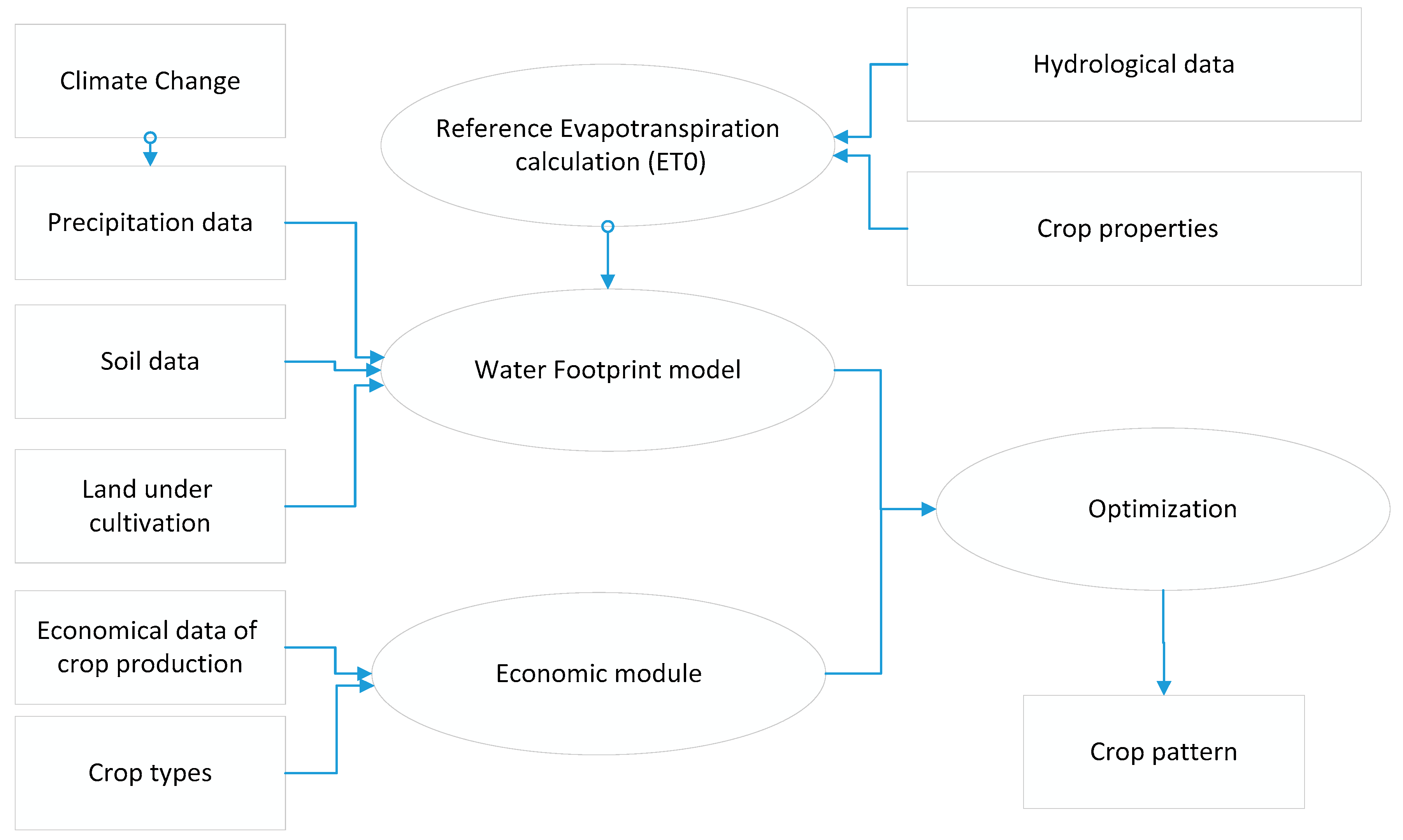
2. Proposed Methodology and Model Structure

Figure 1 presents a schematic relationship between the different modules forming the general modeling scheme for this study. As illustrated, there are three main modules, which calculate the reference evapotranspiration, the water footprint, and the economic measures of the system. An optimization module is also included to address the best cropping pattern and management strategy for reducing the BW to GW ratio. It is specially tailored for any river basin with irrigated agriculture as the main water consumer. It has no limitation on temporal scale, and may efficiently be used in any multi-period problem.

The model is tailored for three different climate conditions, classified as dry, moderate, and wet years. The dry, moderate, and wet years were selected based on the regions’ rainfall data in various drought conditions. To do so, the drought circumstances of each agricultural site was determined based on the monthly data of a 30-year (1985–2015) period using the Standardized Precipitation Index (SPI) [20,21,22]. The SPI indicator can be used for any timescale, simply, and due to its normal distribution, the frequencies of the extreme and severe drought classifications for any region and timescale are consistent [23]. In this study, the drought condition based on SPI was categorized in three general divisions, so-called dry, moderate, and wet. After determining the drought condition of each year, the average rainfall data of moderate years were considered as the monthly rainfall data of the moderate-year scenario, and the similar process for calculating the data for dry and wet years’ scenarios was performed (

Table 1. Calculating the rainfall data of the dry, moderate, and wet years in different scenarios.

Scenarios	Rainfall Data
Dry year	The average of monthly rainfall data of years during the 30-year period in which their SPI is less than or equal to −1
Moderate year	The average of monthly rainfall data of years during the 30-year period in which their SPI is between −1 and 1
Wet year	The average of monthly rainfall data of years during the 30-year period in which their SPI is more than or equal to 1

).

2.1. Evapotranspiration Model (Water Demand Modeling)

Evapotranspiration is defined as the total plant transpiration and evaporation from the land into the atmosphere. To calculate the actual evapotranspiration ($E{T}_a$), Equation (1) is employed [24]:

$$E{T}_a=K_s\ast K_c\ast E{T}_0$$

(1)

where $E{T}_0$. denotes the reference evapotranspiration and can be calculated using the Penman–Monteith equation [24]:

$$E{T}_0=\frac{0.408 \Delta \left(R_n-G\right)+ \gamma \frac{900}{T+273}{u}_2\left(e_s-e_a\right)}{\Delta + \gamma \left(1+0.34 u_2\right)}$$

(2)

$R_n$, $G$, and $\gamma$ in Equation (2) are the net radiation at the crop surface, soil heat flux density, and psychrometric constant, respectively. $e_s$ and $e_a$. stand for the saturation vapor pressure and actual vapor pressure, respectively. Mean daily air temperature at 2 m height, wind speed at 2 m height, and the slope of the vapor pressure curve are expressed by $T$, $u_2$, and $\Delta$, respectively. For a detailed description of the parameters and their calculations, please refer to Alen et al. [24]. Net irrigation depth on day i ($I_i$) is expressed as

$$I_i=\max \left(0,CWR-P_{eff}\right)$$

(3)

where CWR is the crop water requirement, which is equal to $K_c\ast E{T}_c$, and $P_{eff}$ is the net efficient precipitation and can be calculated using Equation (4):

$$P_{eff}=\{\begin{array}{c}\frac{P\times \left(125-0.2\times P\right)}{125}forP\le 250/3 mm\\ 125+0.1 PforP>250/3 mm\end{array}$$

(4)

This paper uses the procedure outlined in CROPWAT [25,26,27] to estimate the yield reductions under the water deficit condition. In fact, Food and Agriculture Organization (FAO) introduced a simple equation, where relative yield reduction is related to the corresponding relative reduction in evapotranspiration (ET). Specifically, the relative yield in response to a reduction in ET is expressed as

$$\left(1-\frac{Y_a}{Y_m}\right)=K_y\left(1-\frac{E{T}_a}{E{T}_c}\right)$$

(5)

where $Y_m$ and $Y_a$ are the maximum and actual yields, $E{T}_c$ and $E{T}_a$ are the maximum and actual evapotranspiration, and $Y_m$ and $Y_a$ are the actual crop yield and maximum expected crop yield, respectively. The yield response factor ($K_y$) represents the effect of a reduction in evapotranspiration on yield losses. It accounts for the complex interactions between crop production and water use, where various biological, physical, and chemical processes may be involved [20]. This relationship has extensively been used and has shown a remarkable validity in quantifying the effects of water deficits on yield. In this study, the procedure was fully coded in AnyLogic [19] for simultaneous simulation of crop water consumption and optimization of cropping patterns for hydro-economic assessment.

2.2. Water Footprint Module

The blue and GW footprint consumption of each crop is calculated using the following relations [10]:

$$W{F}_{proc}=W{F}_{proc,blue}+W{F}_{proc,green}$$

(6)

$$W{F}_{proc,Green}= \frac{CW{U}_{Green}}{Y_a}$$

(7)

$$W{F}_{proc,blue}= \frac{CW{U}_{blue}}{Y_a}$$

(8)

in which crop water consumption (CWU) may be differentiated to BW and GW as follows:

$$CW{U}_{green}=10\times {\displaystyle \sum }_{d=1}^{lgb}E{T}_{green,d}$$

(9)

$$CW{U}_{blue}=10\times {\displaystyle \sum }_{d=1}^{lgb}E{T}_{blue,d}$$

(10)

where lgb is the length of the growing season in days. Equations (9) and (10) for $E{T}_{blue}$ and $E{T}_{green}$. can be rewritten as follows:

$$E{T}_{blue}=\min \left(E{T}_a,IR\right)$$

(11)

$$E{T}_{green}=E{T}_a-E{T}_{blue}$$

(12)

In Equation (11), IR represents the actual irrigation amount to be applied by the farmers. It will be determined based on crop stress factors, where crop yield will vary according to Equation (5).

2.3. Economic Module

Economic Benefit consists of two agricultural gross profits and the cost of crop production. The agricultural gross profit of each region depends on product yield, the land under cultivation, and benefits resulting from crops’ market prices. Here, annual agricultural gross profit for each region is calculated using the following equation:

$$Annual Agri.Benefit={{\displaystyle \sum }}_{\mathrm{i}=1}^{\mathrm{n}}{\mathrm{y}}_{\mathrm{i}}.{\mathrm{A}}_{\mathrm{i}}.{ \mathrm{P}}_{\mathrm{i}}$$

(13)

in which A_i and P_i stand for the area under cultivation and a crops profit per ton for crop i, respectively. The total production cost of each crop, including planting, harvesting, irrigation, and water charge costs, was estimated using data from the national reports of the cost of crop production of the West Azerbaijan, East Azerbaijan, and Kurdistan provinces, Ministry of Agriculture, as of 2014. The data from these regions were used to highlight the possibility of reducing blue water use in favor of recovering Lake Urmia’s water level. Therefore, the results of this study are restricted to these regions and may not be generalized for any other region around the world.

2.4. Optimizing Module

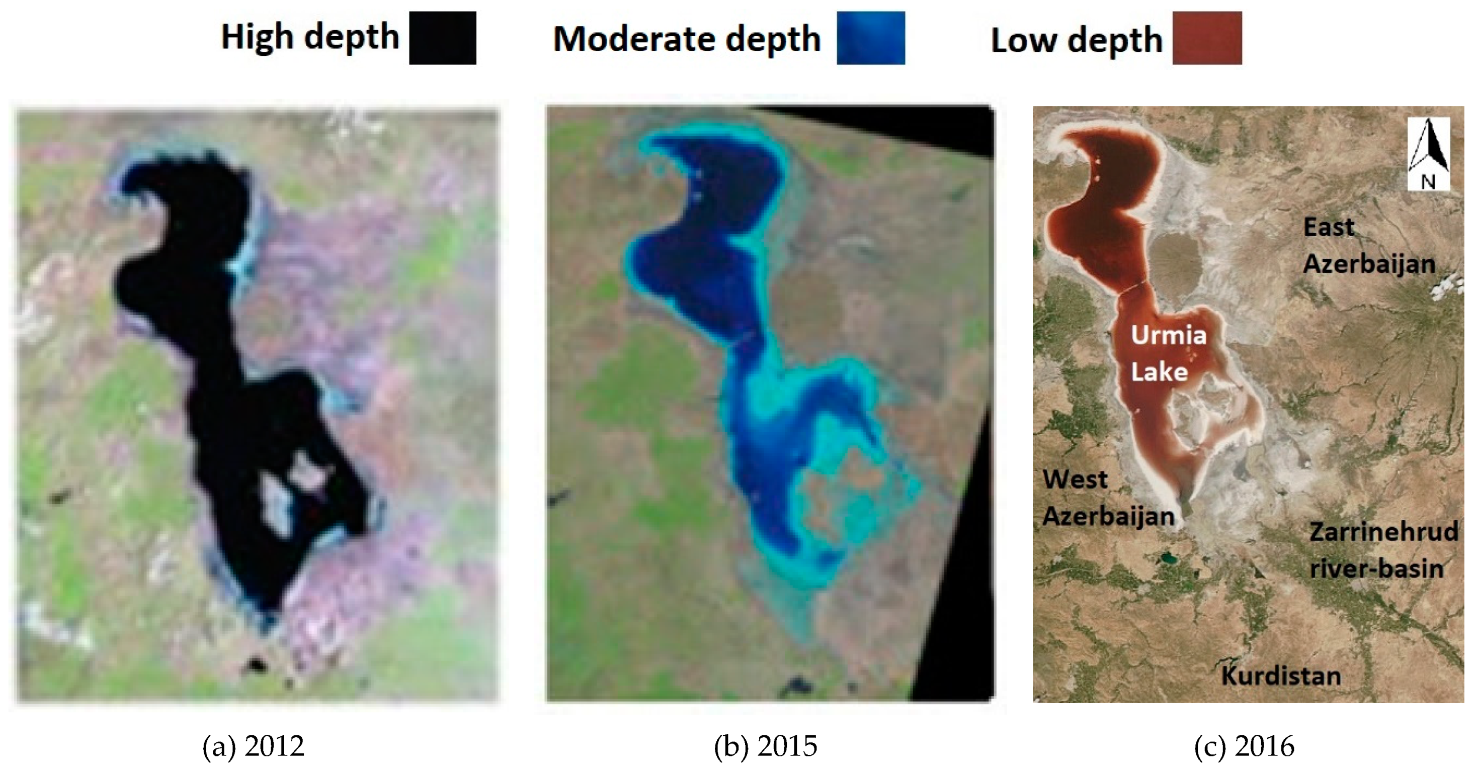
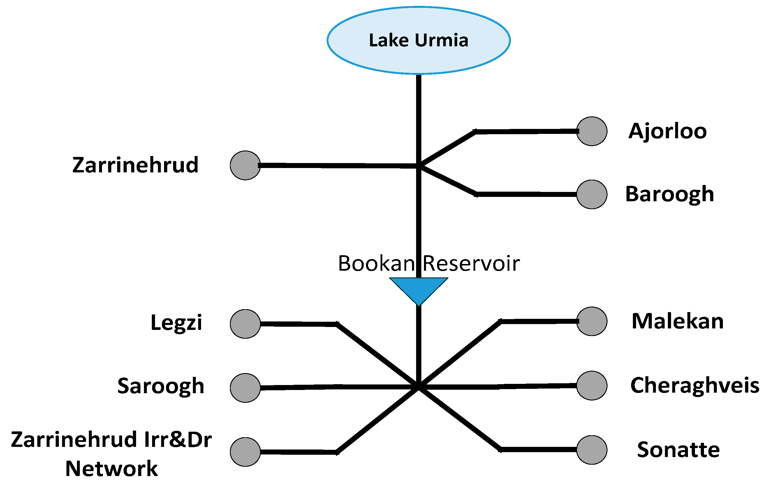
As stated earlier, this study uses the AnyLogic [19] system dynamic platform for system simulation. Unlike most system dynamic simulation models, AnyLogic [19] has its own built-in optimization module, called OptQuest. The OptQuest module considers the simulation model as a black box and uses only the input and output of the model [28]. OptQuest uses a combination of three meta-heuristic search algorithms, namely tabu search, scatter search, and neural network [28,29].

The optimization process consists of repetitive simulations of a model with different parameters. It employs sophisticated algorithms to vary the controllable parameters, from simulation to simulation, to find the optimal parameters for solving a problem. The optimization process may be terminated either when the maximum number of simulations is exceeded or the value of the objective function stops improving significantly. The latter is also known as an automatic stop. The OptQuest engine obtains a sample of the objective function at the end of each simulation. The engine analyzes a sample, modifies the optimization parameters according to its optimization algorithm, and starts a new simulation.

The optimization module intends to propose a desired cropping pattern for maximizing GW to total water use, and net benefit gained by the agricultural sector. It is assumed that the solution may provide more environmental water for lake water level recovery. To reduce the social consequence of the crop reallocation, the model is designed to keep the possible reduction in total cultivated land in each region within an acceptable limit. The optimization model maximizes the two objectives as

$$Max. \left(\frac{W{F}_{green}}{W{F}_{green}+W{F}_{blue}}, NetBenefit\right)$$

(14)

while restricting the variation of land allocated to each crop in each irrigation district from the existing condition within ±25%. As presented, the objective function of the optimization algorithm simultaneously considers the GW to total water use ratio, and the net agricultural benefit. The first term in the objective function is regarded through the footprint perspective, and the second term associates with the regional economy. Although the problem could be solved to provide a set of non-dominated solutions as the Pareto front, this study uses a weighted objective function by assigning different weights to the economic and GW use objectives. For comparison purposes, optimal solutions for the three following weight combinations are presented. The first option (S1) assigns equal weight (0.5, 0.5) to the objectives, the second option (S2) assigns (1, 0) weights to the first (water footprint measure) and second (agricultural profit) objectives, while the third option uses (0, 1) weights. In other words, the second option finds the optimal solution in which the GW use ratio is the only objective, whereas the third one intends to maximize net benefit and disregards the GW ratio as an objective.

3. Case Study

Lake Urmia is located in the north-west part of Iran, which is surrounded by the northern parts of the Zagros Mountains. This lake is one of the largest over-saturated lakes in the world, with characteristics resembling the Great Salt Lake in the western part of the U.S. morphologically, and other aspects such as water chemistry, and sediments [30,31,32]. Due to being a habitat of a species of brine shrimp-aquatic (Artemia Urmiana), this lake can be treated as one of the most important ecological regions for these types of species around the world. Lake Urmia is of priority to be investigated in Iran [33,34]. Besides the above-aforementioned reasons, it has the largest area among all the other lakes in Iran [32]. It is worth mentioning that this lake has been nominated since 1976 as a National Park, and as one of 59 biosphere reserves by UNESCO. It needs to be mentioned that it has been registered in the Ramsar Convention on Wetlands as a wetland of international importance [35,36]. Increasing the rate of water consumption and allocating greater amounts of water to agricultural stakeholders from incoming rivers upstream has caused the level of incoming water to the lake to be reduced, drastically. Figure 2 shows Landsat images of Urmia Lake in 2012, 2015, and 2016, derived from the Urmia Lake restoration program [37,38], and indicates that the southern part of the lake, the Zarrinehrud river-basin, is going to be almost dried up. In Figure 2c, the locations of the Zarrinehrud river-basin, Kurdistan, West Azerbaijan, and East Azerbaijan are presented.

Seventeen main rivers carry water to the Lake Urmia. The Zarrinehrud River has the highest contribution to the Lake hydrology among the existing rivers, and delivers 41 percent of the average annual water to the lake [34]. The Zarrinehrud river-basin supplies irrigation water to nine main agricultural districts (Figure 3). The main products of these irrigation districts are wheat, barley, alfalfa, onions, sugar beets, tomatoes, maize, potatoes, cucumbers, grapes, apples, and peaches.

The agricultural zones in this study are parts of three main irrigation districts in the North West of Iran, for which production cost and gross profit are assumed to remain constant within the district.

Table 2. Agricultural gross profit and cost of crop production in the study area (Figure 2c and Figure 3).

	Agricultural Gross Profit (Tooman/Ha)			Cost of Crop Production (Tooman/Kg)
Crops	Azerbaijan Gharbi	Azerbaijan Sharghi	Kurdistan	Azerbaijan Gharbi	Azerbaijan Sharghi	Kurdistan
Wheat	720,937	661,843	718,257	1200	1300	1155
Barley	804,350	532,382	614,530	1250	1300	920
Alfalfa	1,378,845	775,492	1,394,939	550	700	518
Onion	3,467,196	3,348,287	1,832,148	1800	1500	2400
Sugar beet	2,674,087	2,674,087	2,674,087	270	250	300
Tomato	2,470,183	2,460,549	2,174,020	500	600	578
Maize	977,061	944,719	777,667	900	800	960
Potato	4,298,140	1,087,735	3,973,447	400	350	285
Cucumber	3,506,146	1,481,580	2,406,674	1200	1500	1320
Grapes	2,000,000	2,000,000	2,000,000	2500	2000	2170
Apple	6,500,000	6,500,000	6,500,000	1500	1800	1420
Peach	3,500,000	3,500,000	3,500,000	2200	2000	2000

presents the gross profit and cost of crop production in three districts, namely Kurdistan (Cheraghveis and Sonate), West Azerbaijan (Ajorloo, Baroogh, Zarrinehrud, Saroogh, Legzi, and Zarrinehrud Irr&Dr Network), and East Azerbaijan (Malekan) (Figure 2c). Data were extracted from the official reports from the Ministry of Agriculture as of 2014, and NGOs in each district.

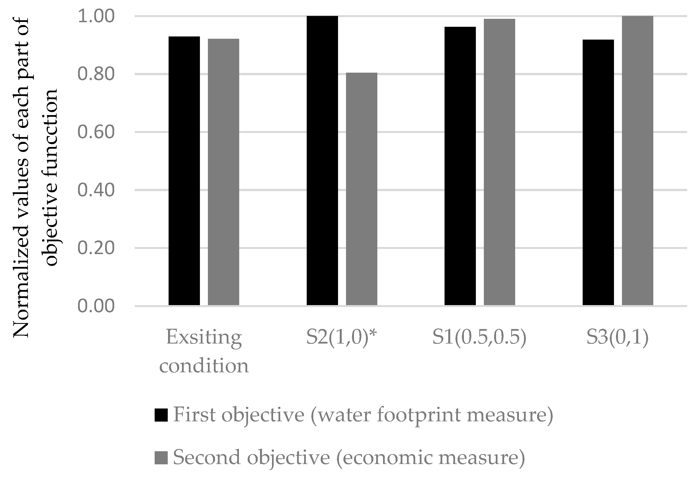
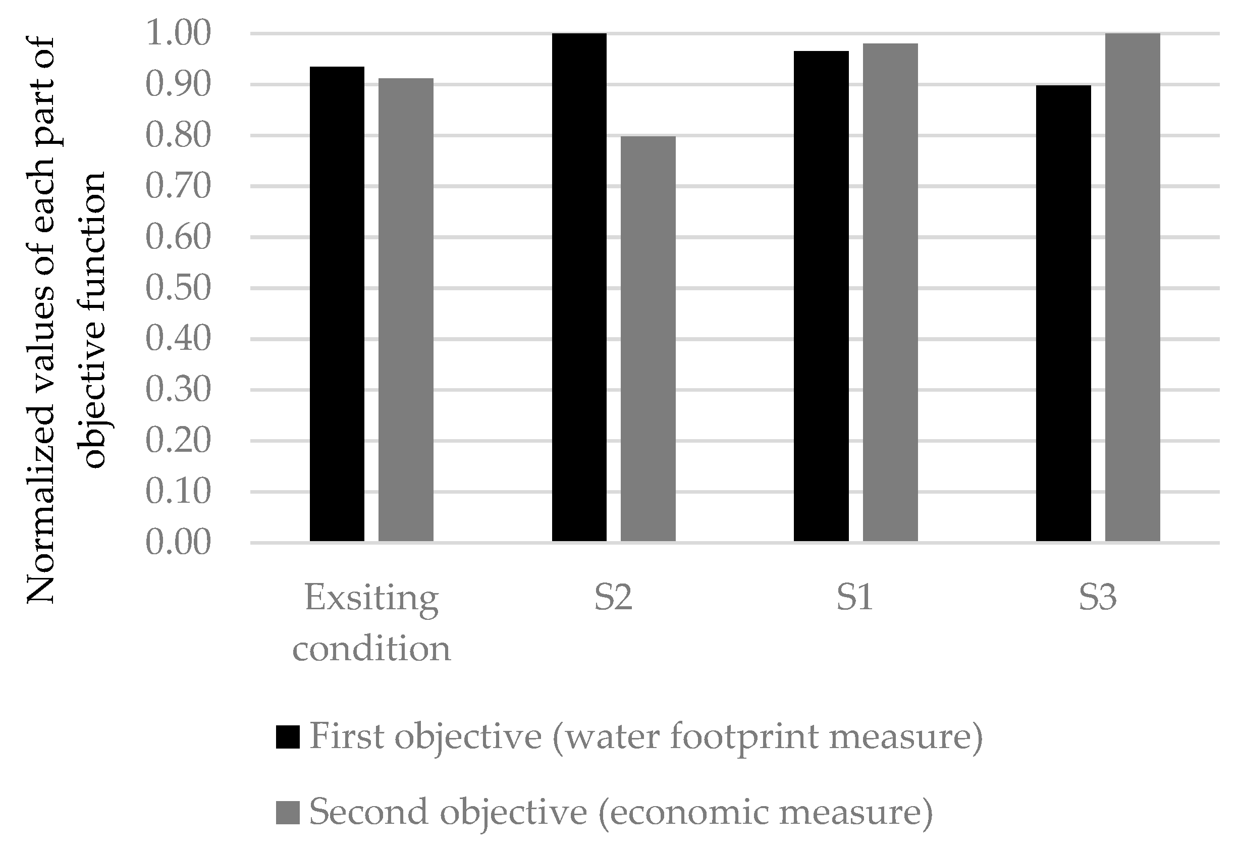
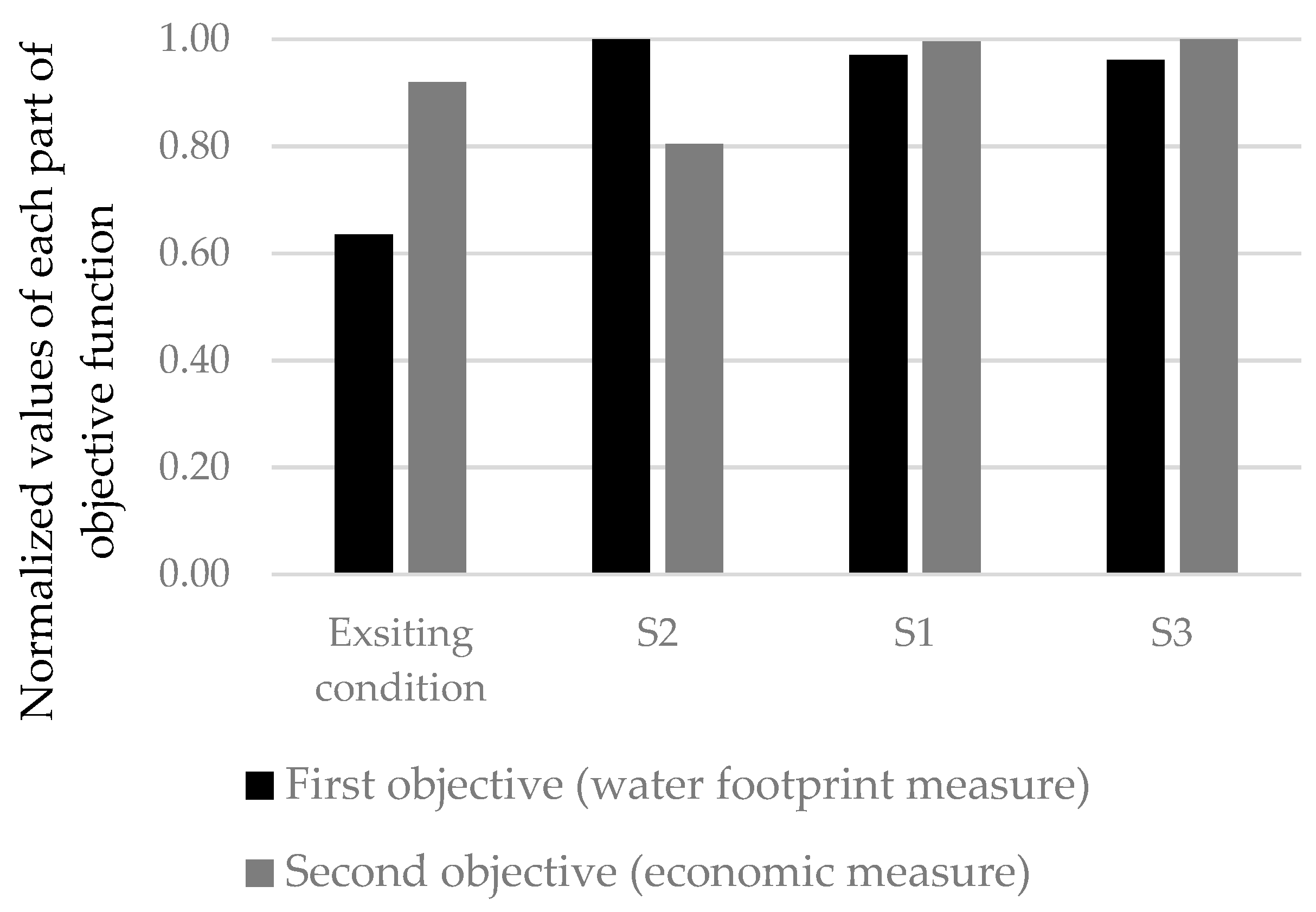
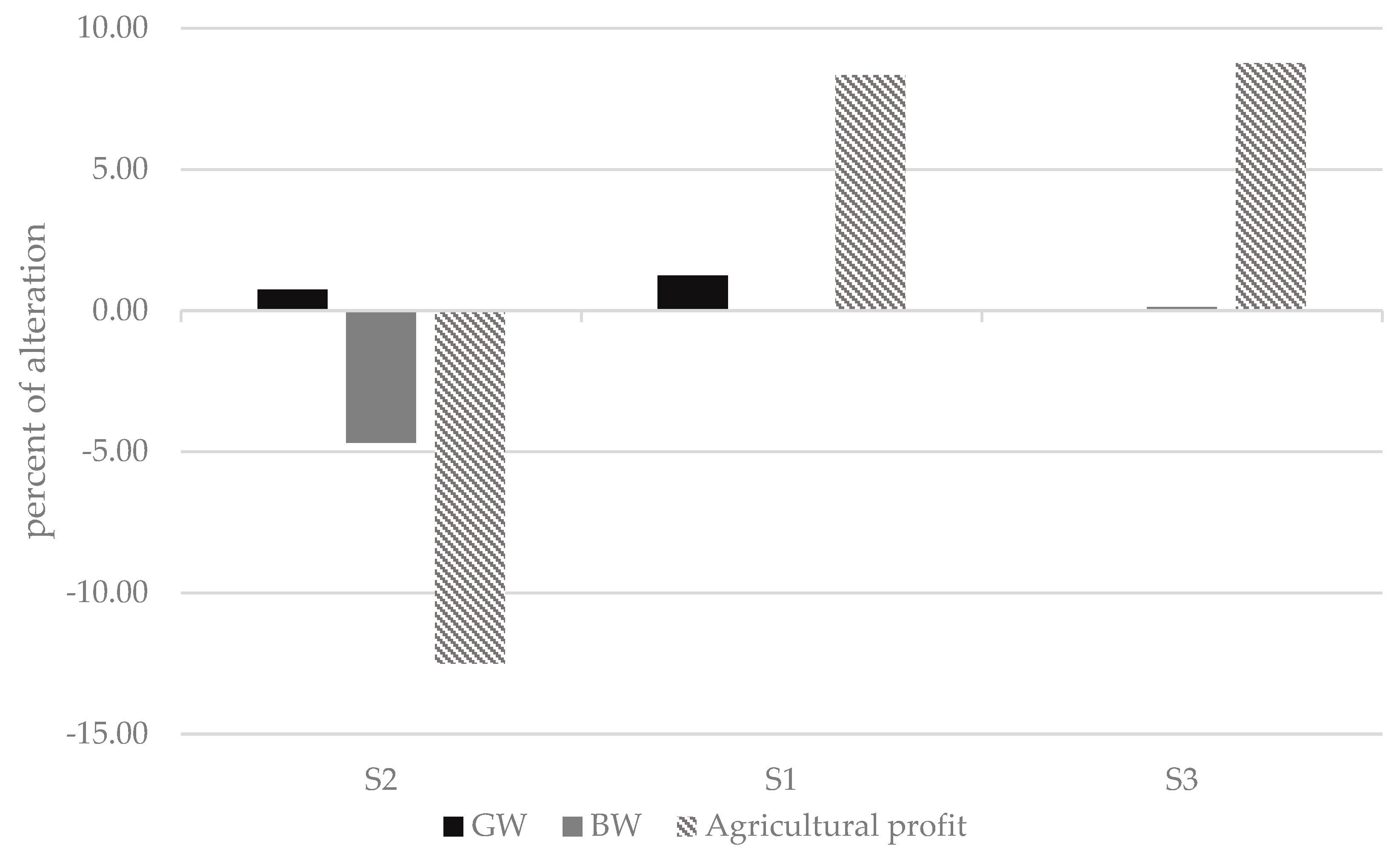
4. Results and Discussion

4.1. Model Setup

To setup the model and verify its performance under any given condition, the model was tested under a specific hypothetical condition for which the optimized solution was known in advance. To do so, a specific crop with the least actual evapotranspiration ($E{T}_a$) was selected from the potential crops cultivated in the region. This selection was based on the regions’ hydrological and geographical data, crops’ properties, and total water consumption of each crop ($E{T}_a$) during a year. Then, a monthly precipitation equal to the monthly evapotranspiration of this crop was assumed for the entire region. In other words, it was assumed that the monthly precipitation in the region was exactly equal to the monthly evapotranspiration of the previously specified crop. The solution was restricted by a constraint in which total land area in all regions should be cultivated. In this case, the solution which maximizes the GW to BW ratio would assign all land area in all 9 irrigation districts to this specific crop, allocating zero hectares to the remaining crops. In fact, the solution to the model allocated the total available land to that crop (i.e., wheat), leaving zero hectares to the remaining nominated crops. This solution is clearly supported by the fact that any other crop will require at least some additional BW during some limited time interval during the growing seasons. The selected crop however can grow exclusively using the available GW resources.

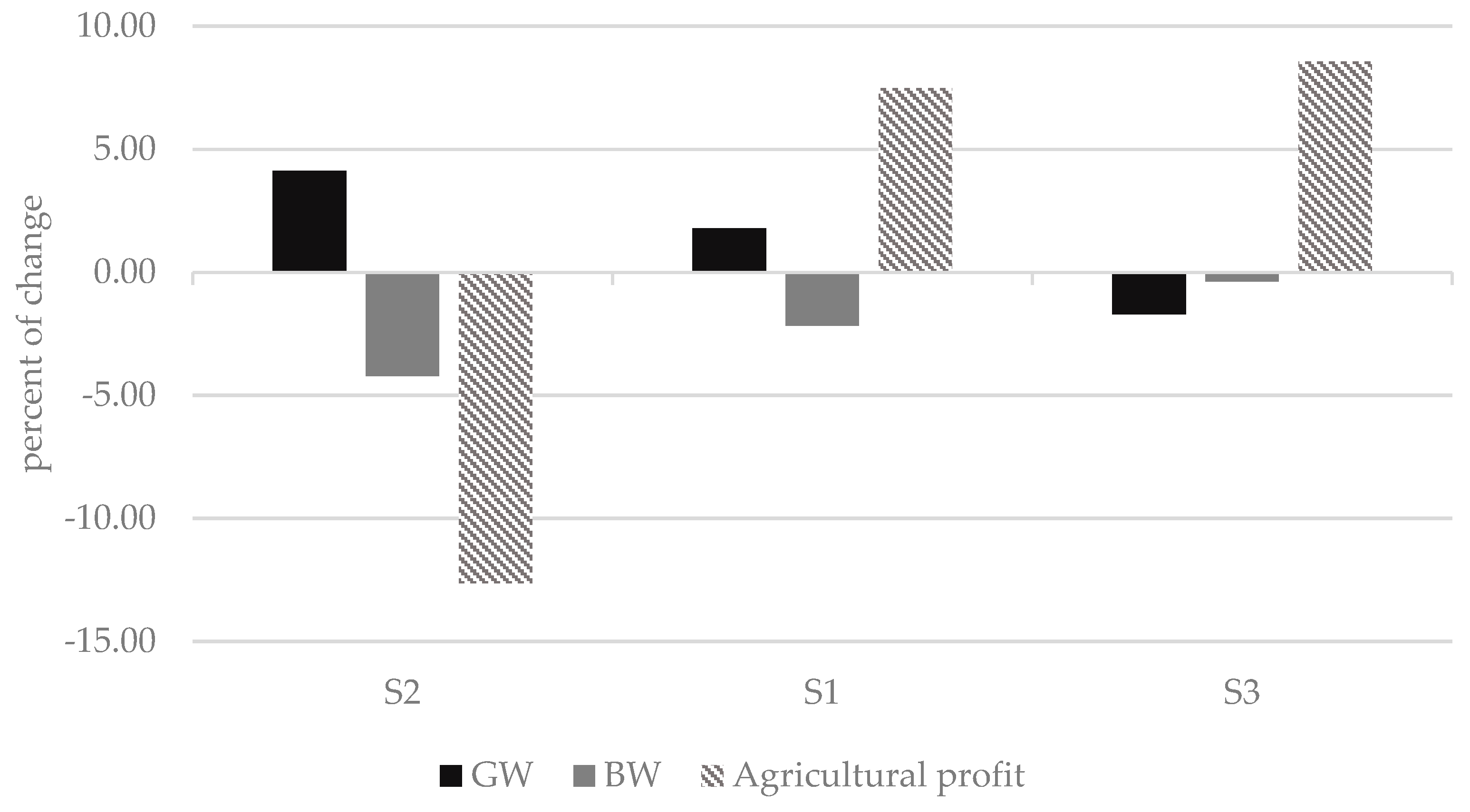
4.2. WF and Agricultural Benefits for the Existing Condition

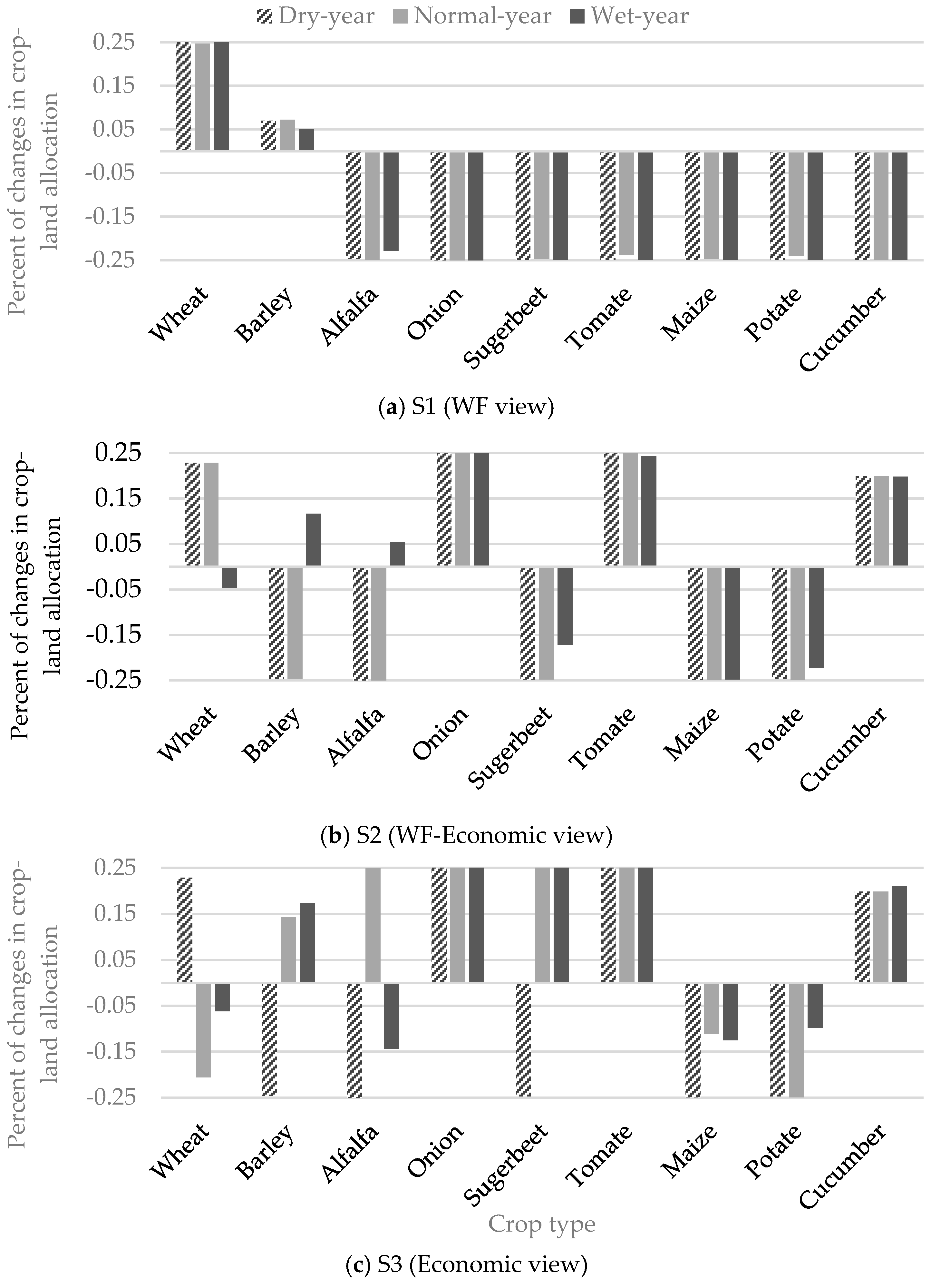
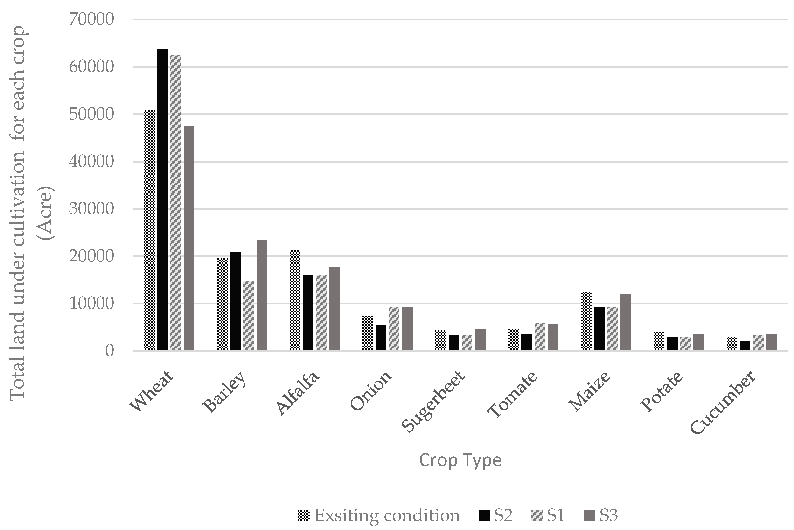
The existing conditions for WF and annual agricultural profit in the region are presented in

Table 3. Agricultural crop production water footprint (WF) and average annual profit for each irrigation district.

Agricultural Sites	WF Consumption for Crop Production (MCM)	Agricultural Profit (Billion Tooman)
Ajorloo	3.2	5.8
Baroogh	6.5	11
Zarrinehrud	71.4	140.1
Legzi	2.0	2.8
Saroogh	4.9	8.3
Zarrinehrud Irr & Dr Network	2.7	3.7
Malekan	12.7	18
Cheraghveis	4.5	7.6
Sonate	9.5	16.3
Sum	117.4	213.6

. The WF for each irrigation district was calculated based on the average lands allocated for each crop in a moderate year. The procedure proposed by FAO [38] was used to calculate the actual evapotranspiration for each crop. As expected, the consumptive water use during a growing season for peaches and alfalfa is the smallest and highest, respectively. In fact, consumptive use of alfalfa exceeds that of peaches by 550 mm per growing season. The spatial variation of the crops’ consumptive use in different irrigation districts of the region was appreciable. In fact, average consumptive use over all crops in the Legzi irrigation district exceeded that of the Zarrinehrud Irrigation and Drainage Network by more than 40%. The regional water footprints were determined according to the amount of the associated region’s evapotranspiration and land allocated to each crop (Table 3).

As presented in Table 3, the agricultural profit for one cubic meter of water for the entire region in the existing condition is approximated as 1820 Iranian Tooman ($0.5). The minimum and maximum values belong to the Zarrinehrud Irrigation and Drainage Network (with 1370 Iranian Tooman) and the Zarrinehrud Irrigation district (with 1960 Iranian Tooman), respectively. As observed, both the values of crop consumptive use and agricultural return per unit of consumed water are very diverse in the region. This diversity may provide a sound environment for the application of this approach to reduce the BW to GW ratio, while maintaining a desired economic condition within the region. Table 3 shows the total WF consumption and agricultural profit in the Zarrinehrud river-basin based on the existing crop pattern. It shows that the Zarrinehrud district has the largest proportion of WF consumption, and consequently of Agricultural profit, among other agricultural districts, due to having the largest cultivated area.

4.3. Crop Pattern

4.3.1. Dry Year Scenario

The model was applied to the regions using specific conditions and data for a typical dry year under the dry-year scenario. The results for three versions of the objective function setup (S1, S2, and S3, as presented in Section 2, Section 3 and Section 4) were compared with that of the existing condition. As presented in Figure 4, under the existing condition, the normalized values of the two conflicting objectives in the bi-objective function (Equation (14)) for the existing condition are 0.93 and 0.91 for the water footprint and economic measures, respectively. Focusing on the water footprint measure and disregarding the economic aspects will increase the water footprint measure to 1.00, while reducing the normalized economic measure to 0.8. This may not be supported by the individual irrigation districts because of major economic losses. As an alternative, disregarding the water footprint measure and focusing on only the economic aspect would result in full economic achievement with the normalized measure of 1.00, while keeping the water footprint normalized measure slightly below 0.93. In other words, the optimized strategy under this scenario may improve the economic measure while keeping the water footprint measure almost unchanged. If equal weight is assigned to both measures in Equation (14), the achievement may look more tempting both sides. In fact, for equal weights of 0.5, the economic measure is close to 0.99, while the footprint measure is above 0.96. Either weights may systematically be changed or multiple objective optimization algorithms [39,40] may be employed if a more precise trade-off and compromise between the objectives is needed.

Figure 5 presents the changes in GW and BW footprints for the S1, S2, and S3 options with those of the existing condition. It also presents the change in total agricultural footprint in comparison with the existing agricultural practice in the region. As illustrated, compared to the original case, the percentage of GW footprint has increased by 4 and 2 percent where weights for water footprint varies from 100% to 50%. When a weight of 100% is assigned to the economic measure of the objective function, the GW footprint shows a 2% reduction compared to the existing condition. It is interesting to observe that when equal weights are assigned to each objective in Equation (14), the GW footprint and economic measure show substantial increases over the existing practice in the region, while the BW footprint is reduced by approximately 3%. This may in fact be assessed as an improvement over the existing condition with no sacrifice by the irrigation districts. For the case of WF perspective, the GW usage increases and BW usage decreases by 4%. Although we have a desirable reduction in the BW to GW ratio, the agricultural profit will be decreased by approximately 13%, which may be severely opposed by the irrigation districts. As the weight of the economic measure in the objective function increases from 50% to 100%, the GW footprint reduces significantly, while the achievement in agricultural profit is minor. A better and more precise tradeoff may be developed by systematically varying the weights.

Figure 6 compares the land allocated to different crops under options S1, S2, and S3 with the existing condition. As expected, land allocation to wheat shows a significant increase over the existing condition for both options S1 and S2. On the other hand, under option S3, the high water consuming crops such as alfalfa, sugar beet, and maize receive more land compared to other options. As stated earlier, land allocated to grapes, apples, and peaches is kept unchanged under different scenarios.

4.3.2. Moderate Year Scenario

To test the performance of the model under the moderate-year condition, data for a typical moderate year was used (moderate-year scenario). The normalized values of the three objective functions set up were compared with that of the existing conditions in Figure 7. The results do not show significant differences between the optimal values of the three objective functions for the dry-year and moderate-year scenarios. In specific, under the existing condition, the normalized values of the two conflicting objectives in the bi-objective function are 0.93 and 0.91 for the water footprint and economic measures, respectively. As expected, disregarding either the economic measure or the water footprint measure will increase the competing objectives (water footprint or economic measure) to 1.00, respectively. Under these conditions, the values of the disregarded objectives will respectively be reduced to 0.80 (for economic measure) and 0.90 (for water footprint measure). Under the S1 scenario, where the water footprint and economic measures receive equal weight (0.5 and 0.5), both objectives show improvement over the existing condition. In particular, the normalized values of the water footprint and economic measures show 3 and 7 percent economic improvements (0.96 and 0.97 compared to 0.93 and 0.90), respectively. Although the economically inferior options may not be supported by the individual farmers, those options superior in both economic and environmental performance may be attractive to farmers and policy developers.

The percent of variations of the GW and BW footprints compared to the existing condition for the moderate-year scenario gives significant negative (−12.5%) and positive (+9%) changes in the economic performance of the system, as expected under S1 and S3 scenarios, where full priorities are assigned to water footprint and economic measures, respectively. Compromising between the two conflicting objectives by assigning equal weights has resulted in a relatively high positive economic gain and GW use with a negative change in BW use, compared to the current practice in the region. Although saving on BW in option S2 is slightly lower than that of the S1 option, the large positive economic gain may make this option superior to S1.

4.3.3. Wet Year Scenario

Figure 8 shows the normalized values of the objective function measures (i.e., economic and water footprint measures) for a typical wet year. Due to the high water availability in a wet year, the difference between the economic and water footprint measures for the S2 and S3 options is not significant. Specifically, while both options result in full economic performance, the S2 option ends up with a slightly better value for the water footprint measure. Under the current practice, although the economic performance of the policy remains approximately the same as the dry and moderate year scenarios, the resulting water footprint measure is disappointing. While the water footprint measure was approximated as 0.93 for typical moderate and dry years, it drops to 0.63 for the typical wet year. This may imply that the current practice is not an appropriate approach in wet years, where water is not scarce. In the S1 option, although GW is efficiently utilized, the economic achievement is well inferior to the S2 and S3 options. In summary, it seems that both the S2 and S3 options may work equally well in wet years, with full economic achievement and excellent utilization of water resources addressed by the water footprint measure.

Figure 9 shows how agricultural profit, as well as GW and BW footprints deviate from the current practice for the S1, S2, and S3 options. While BW consumption is reduced by almost 5 percent in the S1 option, the large decrease in economic performance may not justify its implementation. On the other hand, for both the S2 and S3 options, BW consumption remained unchanged, while an appreciable increase in economic performance is observed. Again, slightly larger GW consumption in the S2 option makes it a competitive alternative. Therefore, one may explore other options adjacent to the S2 option. The S2 option shows that compared to the current practice, a significant improvement in the region’s profit may be achieved without any changes in the water consumption pattern. Again from the water footprint perspective (S2 option), the observed reduction (increase) in BW (GW) consumption is positive for lowering the BW to GW ratio; however, more than 12% reduction in regional profit may not be supported by the agricultural districts.

To be more informative, changes in cropping patterns under the S1, S2, and S3 options for typical dry, wet, and moderate years are presented in Figure 10. This Figure may be utilized as a diagnosis chart for recommending the optimal policy in Lake Urmia, Zarrinehrud river-basin, under each climatological (drought) condition, as classified by dry, moderate, and wet years. Figure 10b recommends partial reductions in planted areas for sugar beet, maize, and potato for all climatological conditions under the S2 option. Under the S1 option, except for wheat and barley, all crops are subject to partial reductions in allocated lands.

Reductions in the BW to GW ratio under the S1 and S2 options for dry, wet, and moderate years are presented in

Table 4. Reduction in the BW to GW ratio under the S1 and S2 options for dry, moderate, and wet years.

Scenarios	S2 (WF View)	S1 (WF-Economic View)
dry-year	−8%	−3.9%
moderate-year	−8.2%	−4%
wet-year	−5.4%	−1.2%

. As observed, compared to the current practice in the region, the BW to GW ratio may be reduced by 1.2 to 8.2 percent under different options and prevailing climatological conditions. For the S2 option, which may not be opposed by the agricultural district, the reduction in the BW to GW ratio may range from 1.2% to 4% for wet to moderate years.

5. Conclusions

This study proposed a modeling approach for systematically redirecting agricultural water management from the BW perspective toward balancing GW and BW use. The proposed hydro-economic model was formulated in the AnyLogic [19] system dynamics platform with a built-in optimization algorithm. The model was employed to assess management strategies, where a compromise between the two objectives, namely regional agricultural profit and BW to GW ratio, was observed. The model was applied to the Zarrinehrud River-basin with nine agricultural districts in Iran. It was observed that, regardless of the decision maker’s priority in valuing the objective functions, the hydro-economics of the region may significantly be improved. For all dry-year, wet-year, and moderate-year conditions, the crop-land allocations would save some BW compared to the current practice, while resulting in a higher regional agricultural return. Although this study assessed only three solutions from the complete set of the optimum non-dominated solutions, the results clearly illustrated that all non-dominated solutions on the Pareto front may be superior to the current practice. More non-dominated solutions may be identified by employing a multi-objective optimization algorithm or systematically changing the weights assigned to the objective functions. This study assumes that the farmers may predict the drought condition of the upcoming year as being dry, wet, or normal. In addition, the study disregards the social behaviour of the farmers, assuming that the best derived policy may be accepted by the farmers for implementation.

References

1. Falkenmark, M.; Rockström, J. The New Blue and Green Water Paradigm: Breaking New Ground for Water Resources Planning and Management; American Society of Civil Engineers: Reston, VI, USA, 2006. [Google Scholar]
2. Falkenmark, M.; Rockström, J. Balancing Water for Humans and Nature: The New Approach in Ecohydrology; Earthscan: Abingdon, UK, 2013. [Google Scholar]
3. Molden, D. Water for Food Water for Life: A Comprehensive Assessment of Water Management in Agriculture; Routledge: Abingdon-on-Thames, UK, 2013. [Google Scholar]
4. Aldaya, M.M.; Allan, J.A.; Hoekstra, A.Y. Strategic importance of green water in international crop trade. Ecol. Econ. 2010, 69, 887–894. [Google Scholar] [CrossRef] [Green Version]
5. Hoekstra, A.Y.; Mekonnen, M.M. The water footprint of humanity. Proc. Natl. Acad. Sci. USA 2012, 109, 3232–3237. [Google Scholar] [CrossRef] [PubMed] [Green Version]
6. Amarasinghe, U.A.; Smakhtin, V. Water productivity and water footprint: Misguided concepts or useful tools in water management and policy? Water Int. 2014, 39, 1000–1017. [Google Scholar] [CrossRef]
7. Tadayon, M.R.; Ebrahimi, R.; Tadayyon, A. Increased water productivity of wheat under supplemental irrigation and nitrogen application in a semi-arid region. J. Agric. Sci. Technol. 2012, 14, 995–1003. [Google Scholar]
8. Falkenmark, M. Land-water linkages: A synopsis. In Land and Water Bulletin: Land and Water Integration and River Basin Management; Food and Agriculture Organization (FAO) of the United Nations: Rome, Italy, 1995; Volume 1, pp. 15–16. [Google Scholar]
9. Mekonnen, M.; Hoekstra, A.Y. National Water Footprint Accounts: The Green, Blue and Grey Water Footprint of Production and Consumption; Unesco-IHE Institute for Water Education: Delft, The Netherlands, 2011. [Google Scholar]
10. Aldaya, M.M.; Chapagain, A.K.; Hoekstra, A.Y.; Mekonnen, M.M. The Water Footprint Assessment Manual: Setting the Global Standard; Routledge: Abingdon-on-Thames, UK, 2012. [Google Scholar]
11. Faramarzi, M.; Abbaspour, K.C.; Schulin, R.; Yang, H. Modelling blue and green water resources availability in Iran. Hydrol. Process. 2009, 23, 486–501. [Google Scholar] [CrossRef]
12. Chapagain, A.K.; Hoekstra, A.Y.; Savenije, H.H.G.; Gautam, R. The water footprint of cotton consumption: An assessment of the impact of worldwide consumption of cotton products on the water resources in the cotton producing countries. Ecol. Econ. 2006, 60, 186–203. [Google Scholar] [CrossRef]
13. Chapagain, A.K.; Hoekstra, A.Y.; Savenije, H.H.G. Water saving through international trade of agricultural products. Hydrol. Earth Syst. Sci. Discuss. 2006, 10, 455–468. [Google Scholar] [CrossRef] [Green Version]
14. Chen, K.; Yang, S.; Zhao, C.; Li, Z.; Luo, Y.; Wang, Z.; Liu, X.; Guan, Y.; Bai, J.; Zhou, Q.; et al. Conversion of Blue Water into Green Water for Improving Utilization Ratio of Water Resources in Degraded Karst Areas. Water 2016, 8, 569. [Google Scholar] [CrossRef]
15. Dumont, A.; Salmoral, G.; Llamas, M.R. The water footprint of a river basin with a special focus on groundwater: The case of Guadalquivir basin (Spain). Water Resour. Ind. 2013, 1, 60–76. [Google Scholar] [CrossRef]
16. Afshar, A.; Neshat, A. Evaluation of Aqua Crop computer model in the potato under irrigation management of continuity plan of Jiroft region, Kerman, Iran. Int. J. Adv. Biol. Biomed. Res. 2013, 1, 1669–1678. [Google Scholar]
17. Chukalla, A.D.; Krol, M.S.; Hoekstra, A.Y. Green and blue water footprint reduction in irrigated agriculture: Effect of irrigation techniques, irrigation strategies and mulching. Hydrol. Earth Syst. Sci. 2015, 19, 4877. [Google Scholar] [CrossRef]
18. El-Gafy, I.K. System dynamic model for crop production, water footprint, and virtual water nexus. Water Resour. Manag. 2014, 28, 4467–4490. [Google Scholar] [CrossRef]
19. AnyLogic. AnyLogic Company: Oakbrook Terrace, IL, USA. (Used Free Trial). Available online: https://www.anylogic.com (accessed on 30 September 2018).
20. McKee, T.B.; Doesken, N.J.; Kleist, J. The relationship of drought frequency and duration to time scales. In Proceedings of the 8th Conference on Applied Climatology, Anaheim, CA, USA, 17–22 January 1993; Volume 17, pp. 179–183. [Google Scholar]
21. McKee, T.B. Drought monitoring with multiple time scales. In Proceedings of the 9th Conference on Applied Climatology, Boston, MA, USA, 15–20 January 1995. [Google Scholar]
22. Hayes, M.J.; Svoboda, M.D.; Wiihite, D.A.; Vanyarkho, O.V. Monitoring the 1996 drought using the standardized precipitation index. Bull. Am. Meteorol. Soc. 1999, 80, 429–438. [Google Scholar] [CrossRef]
23. Edwards, D.C. Characteristics of 20th Century Drought in the United States at Multiple Time Scales; Air Force Inst Of Tech: Wright-Patterson Afb, OH, USA, 1997. [Google Scholar]
24. Cronshey, R.G.; Roberts, R.T.; Miller, N. Urban hydrology for small watersheds (TR-55 Rev.). In Hydraulics and Hydrology in the Small Computer Age; American Society of Civil Engineers: Reston, VI, USA, 1985; pp. 1268–1273. [Google Scholar]
25. Steduto, P.; Hsiao, T.C.; Fereres, E.; Raes, D. Crop Yield Response to Water; FAO: Rome, Italy, 2012; Volume 1028. [Google Scholar]
26. FAO. AQUASTAT—FAO’s Information System on Water and Agriculture; Food and Agriculture Organization: Rome, Italy, 2007; Available online: www.fao.org/nr/water/%0Aaquastat/main/index.stm%0A (accessed on 30 September 2018).
27. FAO. CROPWAT Model; Food and Agriculture Organization: Rome, Italy, 2003. [Google Scholar]
28. Kleijnen, J.P.C.; Wan, J. Optimization of simulated systems: OptQuest and alternatives. Simul. Model. Pract. Theory 2007, 15, 354–362. [Google Scholar] [CrossRef]
29. Laguna, M. OptQuest: Optimization of Complex Systems; White Pap.; OptTek Syst. Inc.: Boulder, CO, USA, 2011; Available online: http//www.opttek.com/white-papers (accessed on 30 September 2018).
30. Kelts, K.; Shahrabi, M. Holocene sedimentology of hypersaline Lake Urmia, northwestern Iran. Palaeogeogr. Palaeoclimatol. Palaeoecol. 1986, 54, 105–130. [Google Scholar] [CrossRef]
31. Ghaheri, M.; Baghal-Vayjooee, M.H.; Naziri, J. Lake Urmia, Iran: A summary review. Int. J. Salt Lake Res. 1999, 8, 19–22. [Google Scholar] [CrossRef]
32. Eimanifar, A.; Mohebbi, F. Urmia Lake (northwest Iran): A brief review. Saline Syst. 2007, 3, 5. [Google Scholar] [CrossRef]
33. Karbassi, A.; Bidhendi, G.N.; Pejman, A.; Bidhendi, M.E. Environmental impacts of desalination on the ecology of Lake Urmia. J. Gt. Lakes Res. 2010, 36, 419–424. [Google Scholar] [CrossRef]
34. Lotfi, A.; Moser, M. A Concise Baseline Report: Lake Uromiyeh; Conservation of Iranian Wetlands Project; IRI Department of Environment, United Nations Development Program: Pardisan Park, Tehran, Iran, 2012. (In English) [Google Scholar]
35. Asem, A.; Eimanifar, A.; Djamali, M.; de los Rios, P.; Wink, M. Biodiversity of the hypersaline Urmia Lake national park (NW Iran). Diversity 2014, 6, 102–132. [Google Scholar] [CrossRef]
36. Urmia Lake Restoration Program. 2015. Available online: http://ulrp.sharif.ir/en (accessed on 29 July 2016).
37. Zeinoddini, M.; Tofighi, M.A.; Vafaee, F. Evaluation of dike-type causeway impacts on the flow and salinity regimes in Urmia Lake, Iran. J. Gt. Lakes Res. 2009, 35, 13–22. [Google Scholar] [CrossRef]
38. Allen, R.G.; Pereira, L.S.; Raes, D.; Smith, M. Crop Evapotranspiration-Guidelines for Computing Crop Water Requirements; FAO Irrigation and Drainage Paper 56; FAO: Rome, Italy, 1998; Volume 300, p. D05109. [Google Scholar]
39. Kaini, P.; Nicklow, J.W.; Schoof, J.T. Impact of climate change projections and best management practices on river flows and sediment load. In Proceedings of the World Environmental and Water Resources Congress 2010: Challenges of Change, Providence, RI, USA, 16–20 May 2010; pp. 2269–2277. [Google Scholar]
40. Afshar, A.; Massoumi, F.; Afshar, A.; Mariño, M.A. State of the art review of ant colony optimization applications in water resource management. Water Resour. Manag. 2015, 29, 3891–3904. [Google Scholar] [CrossRef]
Figure 1. Schematic representation of the proposed modelling scheme using AnyLogic [19].
Agriengineering 01 00005 g001
Figure 2. Landsat images of Urmia Lake [36]. (a) high depth; (b) moderate depth (c) low depth
Agriengineering 01 00005 g002
Figure 3. Schematic diagram of agricultural zones in the Zarrinehrud river-basin.
Agriengineering 01 00005 g003
Figure 4. Normalized values of each objective in the general bi-objective function for the dry-year scenario. * Weights for the first and second objectives.
Agriengineering 01 00005 g004
Figure 5. Percent of changes in green water (GW) and blue water (BW) footprint consumption and agricultural profit compared to the existing condition for the dry-year scenario.
Agriengineering 01 00005 g005
Figure 6. Crop land allocation under the dry-year scenario for different options.
Agriengineering 01 00005 g006
Figure 7. Normalized values of each objective in the general bi-objective function for the moderate-year scenario.
Agriengineering 01 00005 g007
Figure 8. Normalized values of each objective in the general bi-objective function for the wet-year scenario.
Agriengineering 01 00005 g008
Figure 9. Changes in regional profit and GW and BW footprints for the wet-year compared to the current practice.
Agriengineering 01 00005 g009
Figure 10. Cropping patterns under the S1, S2, and S3 options for dry, wet, and moderate years.
Agriengineering 01 00005 g010