Methodology to Solve a Special Case of the Vehicle Routing Problem: A Case Study in the Raw Milk Transportation System

Abstract

This research aims to solve the problem of the raw milk collection and transportation system which can be interpreted as a special case of the vehicle routing problem. In the proposed problem, the factory will send the trucks, multiple fleets composed of several compartments, to collect the raw milk from the raw milk farms. The objective of this research is to minimize the total transportation cost and the trucks’ and tanks’ cleaning costs. The transportation cost directly depends on the fuel usage. The fuel usage occurs during the transportation of the milk and during the waiting times when it arrives at the factory and cannot transfer the raw milk into the production tank. We develop the modified differential evolution algorithm (MDE) to solve the proposed problem. The original process of the Differential Evolution algorithm (DE) has been modified in two folds which are as follows: (1) In the recombination process, the 2nd order of trial vectors has been generated using 3 different strategies and compared with the 1st order trial vector; the better from the 1st and the 2nd order of trial vectors will move to the selection process. (2) The probability function has been used to select the new target vector from one of two sources which are the trial vector and the current target vector so that the worse solution can be accepted in order to increase the diversity of the original DE. The computational result shows that the modified DE (MDE) outperforms the original DE in finding a better solution.

1. Introduction

There are many real-world problems that are hard to solve by using the proposed methods. The vehicle routing problem (VRP) is one of the hard problems which are hard to solve but are very popular problems that researchers are interested in due to their ability to reduce a massive cost for the company. VRP has many variances due to the fact that when the problem is in different business sectors, it usually has some specific conditions which transform the original VRP into a special case VRP that makes it even harder to solve by using the proposed algorithms. An example of the real-world VRP problem is the raw milk transportation problem (RMTP). RMTP needs to use a transportation vehicle that has a cooling system [1]. Moreover, the vehicle which is used in the RMTP usually is composed of three compartments (see Figure 1) which are used to separate the milk from different farms; therefore, the quality of the raw milk will not affect the biochemical reaction which can occur from the mixing of the milks from different farms.

Figure 1 shows the multi-compartment truck which is used to transport the raw milk so the milk from different farms are not mixed and so that the milk retains their quality to be ready to produce high-quality milk products.

Furthermore, due to raw milk having a short shelf life, the transportation has to be executed within a time limitation. The farms that produce the raw milk can do so at only two times: between 05:00–8:00 and 16:00–19:00. Therefore, the production line has to manage good transportation so that all the milk will be transported at the right time. When the time zone is limited, the firm needs to send a truck to deliver the milk within the short timeframe. This generates a waiting queue in front of the production tank which has a limited capacity per round of production. The longer queue generates more fuel usage and finally increases the firm’s cost. This makes the problem become more difficult to solve.

All special characteristics occurring in the RMTP make the raw milk transportation problem more complex than the original VRP problems. These characters are as follows: (1) one vehicle has more than one tank (or it is called a truck with multiple compartments); (2) the quality of milk is maintained by using a cooling system in the transportation but allows the milk from different farms to be mixed but cannot exceed two farms in one tank to control the quality of the milk; (3) there are two times that are possible in which the milk can be collected from the farm; (4) the waiting time of the truck while it is waiting to load the milk into the production line is considered the cost term besides the transportation cost and the tank cleaning cost; (5) it is possible that one truck can go out to collect the raw milk more than one time per day; and (6) the truck can select the start working time which can reduce the waiting time in the queue while it is waiting to load the raw milk into the production line. These attributes make the raw milk transportation a special case of the vehicle routing problem (VRP).

The proposed problem aims to find the lowest operation cost which is generated from the traveling cost, milk storing cost and the cleaning cost of the tank which depends on many parameters such as the distance which is travelled from all routes, the waiting time of the truck waiting to load the milk into the production plant and the number of tanks which are used for all the plans.

This problem turns into a very hard problem to solve. This is due to the fact that the optimal solution which is needed for the problem has to have the following conditions: (1) the solution must generate the lowest transportation cost which depends on the fuel cost. The fuel cost is the cost that the trucks use to transport the raw milk and to operate the cooling system. Hence, the shortest route of the truck needs to be formed while the hold-up time in the queue when the truck is waiting to load the raw milk into the production line must be minimized. The waiting time of the truck depends on its start time and the route that is planned for a comeback in a good time so it has a minimal time to wait in the queue. The wait time consideration makes the problem much harder due to it having a very short time within the time zone; if the truck arrives at the farm later than the time zone, the quality of the milk will reduce and affect the production line. Also important is that (2) the solution must generate the lowest tank cleaning cost; therefore, the three compartments in a tank should be used as much as they can, but it is really free for the truck to collect the milk as much as it can because they are controlled by the time zones in which they are allowed to pick up the raw milk. The time zones mean the truck must arrive at the farms within a limited time. This is because the farmers start to produce the raw milk in two time zones. Also, when the milk is waiting too long in the farms, the quality of the milk will not be good enough for the production line. Therefore, the time zone is set from the duration of the start production time of the raw milk in the farm plus the time that the milk can wait until it is picked up and loaded into the tank.

Due to the difficulty of the proposed problem, an efficient mixed integer programming model is developed for small-size problems. Since the problem considered is an non polynomial hard problem (NP-hard problem), the computational effort, in general, required to find an optimal solution grows exponentially with the size of the problem. In order to find a near optimal solution for bigger problems, a meta-heuristic is developed. The Differential Evolution (DE) is developed to solve this problem. Due to the complexity of the problem, the DE has been improved to increase the search capacity and makes it possible to transform the real number, which is the traditional fashion of DE mechanisms, into the solution of the proposed problem. The DE has been modified in the following ways: (1) it designs the new decoding methods for the proposed problem; (2) it designs three local search techniques to use in the DE to increase the intensification search of the DE and (3) the new selection rule has been invented to make the DE deviate from the local optimal.

This paper is categorized into six sections and organized as following. Section 1 is the introduction which gives the overall outlook, motivation and innovation of the article to the reader. Section 2, the intensive review of the article, will reveal enough background of the problem and method while in Section 3, we present the mixed integer programming representing the propose problem. Section 4 represents the proposed method while Section 5 shows the computational result and framework and Section 6 is the conclusion of the article.

2. Literature Review

In the raw milk transportation industry, Basnet et al. (1999) [2] developed a mixed integer program with some non-linear constraints to solve a joint problem of milk-tanker scheduling and sequencing for the New Zealand dairy industry. Following later, Worasan et al. (2014) [3] developed a mixed integer programming model to solve the raw milk collection problem in the same industry. For the problem where each vehicle contains more than one tank with a heterogeneous capacity to collect raw milk, the raw milk from different collection centers cannot be transferred into the same compartment. In addition, each collection may be visited more than once by more than one vehicle, and each vehicle may visit more than one collection center. The objective of this research is to minimize the total cost consisting of the transportation cost and the costs of cleaning the raw milk tanks. The problem was solved using the CPLEX-MPL software for Windows. However, this exact method is limited to solving the problem only for problems of a small size due to the difficulty of the problem. In order to help deal with this difficulty, Sethanan and Pitakaso (2016) [4] presented the differential evolution algorithm to solve the raw milk transportation problem. The problem which they proposed had the following attributes that differed from the proposed problems which is our main contributions of this paper: (1) the milk from different farms was not allowed in the same tank; (2) the time zone was not considered, but the maximum transportation time was recognized instead; (3) the waiting time in the queue to load the raw milk was not considered; therefore it had no start time for the truck in this article; and (4) the production lead time is not considered [4] but in our algorithm, the production lead time has been considered; therefore the truck has to be well-organized so that it has as less a waiting time as possible. These research projects used differential evolution algorithms to solve the problem. The DE has been modified by adding the reincarnation and survival processes in the original DE, and the computational result shows that these two processes has benefits to add in the original DE.

The case study which is presented in this article is the special case of the vehicle routing problem (VRP). VRP aims to find a set of routes for the visiting plan of all the customers from the depot that generate the minimum traveling cost. All customers must be travelled through by one route. There are many varieties of subproblems of VRP, such as vehicle routing with a time window (VRPTW) where the customer’s preferred time to be visited is considered, VRP with pickup and delivery consideration and VRP with split delivery (VRPSD), which is the VRP problem where the customer can be visited by more than one vehicle. VRP can be also integrated with other types of problems such as scheduling problems [5] and production planning problems [4]

De et al. (2015) [5] presented the complex ship routing and scheduling problem where the multiple ports, the multiple time windows within a planning horizon and the varying demand and supply at different ports were added to the model. The particle swarm optimization for composite particle (PSO-CP) was presented to solve the proposed problem. Later on, De et al. (2016) [6] formulated a sustainable ship routing and scheduling problem by adding carbon emission, fuel consumption and fuel cost constraints and then applied the PSO-CP to solve the proposed problem. Dominguez et al. (2016) [7] presented a hybrid algorithm that integrated the biased randomized versions of vehicle routing and packing heuristics within a large neighborhood search metaheuristic framework to solve the two-dimensional loading vehicle routing problem with clustered backhauls (2L-VRPB). Can and Can (2016) [8] presented the combination of an ant colony optimization (ACO) and variable neighborhood search (VNS) to solve the vehicle routing problem with simultaneous pickup and delivery. This article focuses on improving the efficiency of the ACO and VNS; therefore, the new combination method has been tested with the standard bench marking problem instances, and the result of the proposed method is outstanding compared with others.

De et al. (2017) [9] presented a mixed integer non-linear programming model for the various scheduling and routing, loading/unloading and vessel capacity constraints. The fuel consumption, time windows and service levels were also integrated in the model. De et al. (2019) [10] extended De et al. (2017) [9] from a single objective to a multi-objective model. The model was used to optimize the total fuel consumed and the carbon emissions from each vessel. Two novel algorithms were presented which are (1) nondominated sorting genetic algorithm II (NSGA-II) and multi-objective particle swarm optimization. De et al. (2018) [11] formulated the mathematical model for the dynamic ship berth allocation problem for a container handling port. The model considered the fuel costs that connect to the waiting time and operational time of the docked vessel and the hiring of the quay cranes to load/unload the containers. A chemical reaction optimization algorithm is proposed to solve the problem in a large-scale realistic environment.

In the agricultural business, especially in Thailand, there is a limitation of the road and area, as big trucks cannot access and serve some farmers. The parking area for big trucks are needed, and small trucks will be used to reach the farmers. Then, the raw milk is loaded from a small truck to a big truck in the parking area; when this occurs, the problem is called the truck and trailer routing problem (TTRP) [12,13]. TTRP is sometimes defined a generalized assignment problem (GAP) [14]. Following from this, Chao (2002) [15] assigned the vehicles to farmers considered as customers in order to minimize the total distance of all vehicles travelled. In this research, the linear relaxation of the GAP formulation and the Tabu Search is used to find the solution of the proposed problem. The Tabu search algorithm has been used to solve the problem by 16. Scheuerer (2006) [16] in which the author developed two constructive heuristics and a Tabu search algorithm to solve the TTRP. Tan et al. (2006) [17] proposed an evolutionary algorithm to solve the TTRP which has two objective functions that minimized the number of trucks and minimized the routing cost. Hoff and Løkketangen (2007) [18] developed a Tabu search algorithm to solve the milk collection problem, the TTRP. Besides the Tabu search technique that has been wildly used to solve the TTRP, the raw milk transportation problem, others metaheuristics such as genetic algorithm (GA), tabu search (TS), Particle swarm optimization (PSO), Ant Colony Optimization (ACO) and simulated annealing (SA) have been used to solve combinatorial problems [19]

The differential evolution (DE) was first introduced in 1997 [20]. Due to the effectiveness of DE, it has been successfully used in many types of combinatorial optimizations such as assembly line balancing [21,22], manufacturing problems [2], transportation problems [23], vehicle routing problems [24,25] and the capacitated VRP with the flexibility of mixing pickup and delivery services [26].

The general procedure of DE is comprised of four steps which are (1) generate initial solution, (2) perform mutation process, (3) perform recombination process and (4) perform selection process. Additionally, Sethanan and Pitakaso (2016) [27] created two additional steps more from the original DE process, which are the re-incarnation process and survival process. This article added these two steps to increase the performance of the original DE. The DE can be improved by adding more steps into the original steps and other techniques such as use various mutation and recombination formula [21,22,28], add effective local search techniques [27], add the best vector reproduction process [29], develop new decoding method which is combined with ant colony optimization [30]. Therefore, in this article, the DE has been improved in following ways so that the effectiveness of DE is increased: (1) provided an effective decoding method; (2) presented new rules of the selection process to let DE escape from the local optimal; and (3) used 3 different local searches so that the DE has intensive search efficiency.

3. Problem Description and Mathematical Formulation

The VRP models in the case study are not the same as the other general models. This is because there are limitations of (1) traveling time in order to get the raw milk transporting truck returned to the plant at about the same time, (2) the time for transferring the raw milk from the raw milk farm to the raw milk transporting truck, (3) the time used for transferring the raw milk from the truck to the plant tank which had limited capacity, (4) the time required for cleaning the truck and the tank, and (5) the number of trucks carrying raw milk. For receiving raw milk, there were two periods of time windows—8 h or 480 min for each period.

From Figure 2, when the travelling starts from the milk plant to the raw milk farm, the decision variable is $X_{rtij}$ r is a traveling route, t is truck, i is the milk plant and j is the raw milk farm of relevance. If there was travelling, $X_{rtij}$ becomes 1 if no travelling occurred; otherwise, $X_{rtij}$ was 0. When the truck carrying raw milk travels to the raw milk farm, there is raw milk transferred from the raw milk farm to the milk truck in each compartment c, with the transfer rate of 10 ton/hour. If the milk is completely filled to the 3 compartments, the truck then returns to the plant. If the milk volume has not reached the full truck capacity, the truck has to travel to the next raw milk farm to fill the truck capacity before returning to the plant. When the truck carrying the raw milk travels to the milk plant, the raw milk is transferred from the truck to the plant tank. The tank capacity is 17 ton with the transferring rate of 10 ton/hour. During this process, if there is another truck coming to the plant, the next trucks have to wait with the cost for storing milk at 90 baht/hour. For example, if there are two trucks coming to the production line at the same time, each of which is carrying a full capacity of 15 and 12 tons respectively, the 12 tons truck is allowed to load first; therefore the 15 tons truck needs to wait 1 h 12 min (10 tons/hour). This 1 h 12 min generate 108 baht of milk storing cost during the waiting. When the plant tank has been completely filled, the raw milk transferring from truck to plant process stops and the raw milk processing starts at the rate of 10 ton/hour. When the transferring of the raw milk process finishes, the plant tank cleaning is done at the cost of 2000 baht/time. When the plant milk tank has been cleaned, the raw milk transferring from truck to plant tank continues as normal and the cleaned truck compartment then moves to receive raw milk from a raw milk farm. From this regulation, the solution must have the shortest route, shortest waiting time of the truck and fewest vehicles that are used; therefore the minimum cost is generated.

The following mathematical model is the equation to finding the minimum cost in transporting the raw milk, including the cost of traveling, cost of cleaning a raw milk carrying truck, cost of cleaning the plant milk tank and cost of waiting to maintain the quality of the milk before transferring the milk to the plant tank. The parameters and decision variables are the following:

Indices

s (time)	Shifting of the production line (s = 1..S)
z (timezone)	Time zone (z = 1..Z)
i	Raw milk farm (i = 1..I)
j	Raw milk farm (j = 1..J)
t	Truck label (t = 1..T)
c (compartment)	Label of compartment of truck (c = 1..C)
r (round)	Round of Truck (r = 1..R)

Parameter

P	Production rate (ton/hours)
MX	Capacity of the production tank (ton)
WC	Waiting cost of the truck before it can load (bath/hours)
CT	Cleaning cost of the production tank (bath/time)
CTI	Cleaning time of the production tank (hours)
CTC	Cleaning time of a compartment in truck (hours)
$V_{tc}^{CAP}$	Capacity of compartment c in truck t
$C_{tc}^l$	Cleaning cost of compartment c in truck t
$M_k$	Amount of milk available at milk raw milk farm k
$S_z^T$	Start time of windows z
$E_z^T$	End time of windows z
LRT	Loading rate of milk into the truck (ton/hours)
LRA	Loading rate of milk into the production tank (ton/hours)
FR	Driving speed of truck (km/hours)
$D_{ij}$	Distance of raw milk raw milk farm i to j
SPT1	Start time of the first loading in a day
MN	Maximum number of milk raw milk farms that can mix the milk into the same compartment
$C_t^{OR}$	Consume rate of truck t (bath/km)

Decision Variables

$X_{rtij}$	1 if round r of truck t traveling from i to j 0 otherwise
$V_{rtc}$	1 if compartment c is used in round r truck t 0 otherwise
$T_s^E$	1 if shifting s need to clean the tank 0 otherwise
$T_{rst}^Z$	1 if amount of milk that is delivered in round r truck t shifting s greater than zero 0 otherwise
$T_{rtz}^W$	1 if round r truck t using time windows zone z 0 otherwise
$G_{rtck}$	1 if amount of milk that is delivered from raw milk farm k in round r truck t compartment c greater than zero 0 otherwise
$A_{rtk}$	1 if amount of milk from raw milk farm that is delivered in round r truck t is greater than zero 0 otherwise
$U_{rtk}$	Dummy variable of round r truck t milk raw milk farm k for subtour elimination constraint
$W_{rts}$	Waiting time of operation round t truck t shifting s
$V_{rts}^S$	Amount of milk that is delivered in round r truck t to shifting s
$V_{rtck}^K$	Amount of milk that is delivered from milk raw milk farm k in round r truck t compartment c
$B_{rt}^T$	Start traveling time of round r truck t
$W_{rt}^T$	Waiting time to start round r truck t
$E_{rt}^{TIME}$	End time of the time windows of round r truck t
$P_s^R$	Processing time of shifting s
$S_s^{LR}$	Start loading time of shifting s
$E_s^{PT}$	End processing time of shifting s
$A_{rts}^{RT}$	Arrive time of round r truck t shifting s
$E_{rt}^R$	End traveling time of round r truck t
$F_{rt}^{ER}$	Final end of tour and production of round r truck t
$A_{rtk}^{RK}$	Arrival time of round r truck t at milk raw milk farm k
$F_{rtk}$	Finish time at milk raw milk farm k of round r truck t
$M^{BIG}$	Large number
$S_{rt}^{TIME}$	Start time of the time windows of round r truck t

Objective Function

Minimize

$${\displaystyle {\displaystyle \sum }_{i=1}^I}{\displaystyle {\displaystyle \sum }_{j=1}^J}{\displaystyle {\displaystyle \sum }_{t=1}^T}{\displaystyle {\displaystyle \sum }_{r=1}^R}{D}_{ij}{X}_{rtij}{C}_t^{OR}+{\displaystyle {\displaystyle \sum }_{c=1}^C}{\displaystyle {\displaystyle \sum }_{t=1}^T}{\displaystyle {\displaystyle \sum }_{r=1}^R}{V}_{rtc}{C}_{tc}^l+ {\displaystyle {\displaystyle \sum }_{s=1}^S}{\displaystyle {\displaystyle \sum }_{t=1}^T}{\displaystyle {\displaystyle \sum }_{r=1}^R}{W}_{trs}{W}^C + {\displaystyle {\displaystyle \sum }_{s=1}^S}{T}_s^E{C}^T$$

(1)

Constraints

$$\begin{array}{cc}{\displaystyle {\displaystyle \sum }_s^S}{V}_{rts}^S={\displaystyle {\displaystyle \sum }_k^K}{\displaystyle {\displaystyle \sum }_c^C}{V}_{rtck}^K\hfill & \hspace{1em}\hspace{1em}\hspace{1em}\hspace{1em}\hspace{1em}\forall r,t=1..R,T\end{array}$$

(2)

$$\begin{array}{cc}{V}_{rts}^S\le T_{rst}^Z{M}^{BIG}\hfill & \hspace{1em}\hspace{1em}\hspace{1em}\hspace{1em}\hspace{1em}\forall r,t,s=1..R,T,S\end{array}$$

(3)

$$\begin{array}{cc}{V}_{rts}^S\le T_s^E{M}^{BIG}\hfill & \hspace{1em}\hspace{1em}\hspace{1em}\hspace{1em}\hspace{1em}\forall r,t,s=1..R,T,S\end{array}$$

(4)

$$\begin{array}{cc}{T}_{s-1}^E\le T_s^E\hfill & \hspace{1em}\hspace{1em}\hspace{1em}\hspace{1em}\hspace{1em}s=2\end{array}$$

(5)

$$\begin{array}{cc}{T}_{r-1st}^Z>{\displaystyle {\displaystyle \sum }_{b=\left(s-a\right)}^1}{T}_{rst}^Z\hfill & \hspace{1em}\hspace{1em}\hspace{1em}\hspace{1em}\hspace{1em}\forall r,t=1..R,T, s=2..S\end{array}$$

(6)

$$\begin{array}{cc}{S}_s^{LR}\ge E_{s-1}^{PT}\hfill & \hspace{1em}\hspace{1em}\hspace{1em}\hspace{1em}\hspace{1em}\forall s=2..S\end{array}$$

(7)

$$S_1^{LR}\ge S_{}^{PT1}$$

(8)

$$\begin{array}{cc}{E}_s^{PT}\ge S_s^{LR}+{\displaystyle {\displaystyle \sum }_{t=1}^T}{\displaystyle {\displaystyle \sum }_{r=1}^R}\frac{V_{rts}^S}{L^{RA}}+{\displaystyle {\displaystyle \sum }_{t=1}^T}{\displaystyle {\displaystyle \sum }_{r=1}^R}\frac{V_{rts}^S}{p}+C^{TI}\hfill & \hspace{1em}\hspace{1em}\hspace{1em}\hspace{1em}\hspace{1em}\forall s=1..S\end{array}$$

(9)

$$\begin{array}{cc}{A}_{rts}^{RT}{T}_{rst}^Z\le S_s^{LR}\hfill & \hspace{1em}\hspace{1em}\hspace{1em}\hspace{1em}\hspace{1em}\forall r,t,s=1..R,T,S\end{array}$$

(10)

$$\begin{array}{cc}{E}_{rt}^R={\displaystyle {\displaystyle \sum }_{s=1}^S}{A}_{rts}^{RT}{T}_{rst}^Z\hfill & \hspace{1em}\hspace{1em}\hspace{1em}\hspace{1em}\hspace{1em}\forall r,t=1..R,T\end{array}$$

(11)

$$\begin{array}{cc}{W}_{rts}= S_s^{LR}-A_{rts}^{RT}\hfill & \hspace{1em}\hspace{1em}\hspace{1em}\hspace{1em}\hspace{1em}\forall r,t,s=1..R,T,S\end{array}$$

(12)

$$\begin{array}{cc}{F}_{rt}^{ER}={\displaystyle {\displaystyle \sum }_{s=1}^S}[S_s^{LR}+{\displaystyle {\displaystyle \sum }_{t=1}^T}{\displaystyle {\displaystyle \sum }_{r=1}^R}\frac{V_{rts}^S}{L^{RA}}+{\displaystyle {\displaystyle \sum }_{c=1}^C}{V}_{rtc}{C}^{TC}]T_{rst}^Z\hfill & \hspace{1em}\hspace{1em}\hspace{1em}\hspace{1em}\hspace{1em}\forall r,t=1..R,T\end{array}$$

(13)

$$\begin{array}{cc}{B}_{rt}^T=F_{r-1t}^{ER}+W_{rt}^T\hfill & \hspace{1em}\hspace{1em}\hspace{1em}\hspace{1em}\hspace{1em}\forall r,t=1..R,T\end{array}$$

(14)

$$\begin{array}{cc}{B}_{1t}^T= W_{1t}^T\hfill & \hspace{1em}\hspace{1em}\hspace{1em}\hspace{1em}\hspace{1em}\forall t=1..T\end{array}$$

(15)

$$\begin{array}{cc}{\displaystyle {\displaystyle \sum }_{c=1}^C}{\displaystyle {\displaystyle \sum }_{t=1}^T}{\displaystyle {\displaystyle \sum }_{r=1}^R}{V}_{rtck}^K=M_k\hfill & \hspace{1em}\hspace{1em}\hspace{1em}\hspace{1em}\hspace{1em}\forall k=1..K\end{array}$$

(16)

$$\begin{array}{cc}{\displaystyle {\displaystyle \sum }_k^K}{V}_{rtck}^K\le V_{tc}^{CAP}\hfill & \hspace{1em}\hspace{1em}\hspace{1em}\hspace{1em}\hspace{1em}\forall r,t,c=1..R,T,C\end{array}$$

(17)

$$\begin{array}{cc}{\displaystyle {\displaystyle \sum }_{s=1}^S}{T}_{rst}^Z\le 1\hfill & \hspace{1em}\hspace{1em}\hspace{1em}\hspace{1em}\hspace{1em}\forall r,t=1..R,T\end{array}$$

(18)

$$\begin{array}{cc}{V}_{rtck}^K\le G_{rtck}{M}^{BIG}\hfill & \hspace{1em}\hspace{1em}\hspace{1em}\hspace{1em}\hspace{1em}\forall t,k,c=1..T,K,C, r=2..R\end{array}$$

(19)

$$\begin{array}{cc}{A}_{rtk}\ge G_{rtck}\hfill & \hspace{1em}\hspace{1em}\hspace{1em}\hspace{1em}\hspace{1em}\forall r,t,c=1..R,T,C, k=2..K\end{array}$$

(20)

$$\begin{array}{cc}{G}_{rtck}\le V_{rtc}\hfill & \hspace{1em}\hspace{1em}\hspace{1em}\hspace{1em}\hspace{1em}\forall r,t,c,k=1..R,T,C, K\end{array}$$

(21)

$$\begin{array}{cc}{\displaystyle {\displaystyle \sum }_{m=1}^M}{X}_{rtkm}+{\displaystyle {\displaystyle \sum }_{n=1}^N}{X}_{rtnk}=2\times A_{rtk}\hfill & \hspace{1em}\hspace{1em}\hspace{1em}\hspace{1em}\hspace{1em}\forall r,t=1..R,T, m,n,k=2..M,N, K\end{array}$$

(22)

$$\begin{array}{cc}{\displaystyle {\displaystyle \sum }_{m=1}^M}{\displaystyle {\displaystyle \sum }_{t=1}^T}{\displaystyle {\displaystyle \sum }_{r=1}^R}{X}_{rtkm}\ge 1\hfill & \hspace{1em}\hspace{1em}\hspace{1em}\hspace{1em}\hspace{1em}\forall k=2..K\end{array}$$

(23)

$$\begin{array}{cc}{\displaystyle {\displaystyle \sum }_{n=1}^N}{\displaystyle {\displaystyle \sum }_{t=1}^T}{\displaystyle {\displaystyle \sum }_{r=1}^R}{X}_{rtnk} \ge 1\hfill & \hspace{1em}\hspace{1em}\hspace{1em}\hspace{1em}\hspace{1em}\forall k=2..K\end{array}$$

(24)

$$\begin{array}{cc}{\displaystyle {\displaystyle \sum }_{i=1}^I}{X}_{rtik}-{\displaystyle {\displaystyle \sum }_{i=1}^I}{X}_{rtki}=0\hfill & \hspace{1em}\hspace{1em}\hspace{1em}\hspace{1em}\hspace{1em}\forall r,t=1..R,T, k=2.., K\end{array}$$

(25)

$$\begin{array}{cc}{\displaystyle {\displaystyle \sum }_{k=1}^K}{G}_{rtck}{V}_{rtck}^K\le M^N\hfill & \hspace{1em}\hspace{1em}\hspace{1em}\hspace{1em}\hspace{1em}\forall r,t=1..R,T, c=2.., C\end{array}$$

(26)

$$\begin{array}{cc}{A}_{rtk}^{RK}={\displaystyle {\displaystyle \sum }_{i=1}^I}{F}_{rti}{X}_{rtik}+{\displaystyle {\displaystyle \sum }_{i=1}^I}\frac{D_{ik}{X}_{rtik}}{F^R}\hfill & \hspace{1em}\hspace{1em}\hspace{1em}\hspace{1em}\hspace{1em}\forall r,t,k=1..R,T,K,i\ne k,i=1\end{array}$$

(27)

$$\begin{array}{cc}{A}_{rtk}^{RK}={\displaystyle {\displaystyle \sum }_{i=1}^I}{F}_{rti}{X}_{rtik}+{\displaystyle {\displaystyle \sum }_{i=1}^I}\left[B_{rt}^T+\frac{D_{ik}{X}_{rtik}}{F^R}\right]\hfill & \hspace{1em}\hspace{1em}\hspace{1em}\hspace{1em}\hspace{1em}\forall r,t,k=1..R,T,K,i\ne k,i=1\end{array}$$

(28)

$$\begin{array}{cc}{F}_{rtk}=A_{rtk}^{RK}+{\displaystyle {\displaystyle \sum }_{c=1}^C}\frac{V_{rtck}^K}{L^{RA}}\hfill & \hspace{1em}\hspace{1em}\hspace{1em}\hspace{1em}\hspace{1em}\forall r,t,k=1..R,T,K\end{array}$$

(29)

$$\begin{array}{cc}{A}_{rtk}^{RK}\ge S_{rt}^{TIME}\hfill & \hspace{1em}\hspace{1em}\hspace{1em}\hspace{1em}\hspace{1em}\forall r,t=1..R,T, k=2.., K\end{array}$$

(30)

$$\begin{array}{cc}{F}_{rtk}\le E_{rt}^{TIME}\hfill & \hspace{1em}\hspace{1em}\hspace{1em}\hspace{1em}\hspace{1em}\forall r,t=1..R,T, k=2.., K\end{array}$$

(31)

$$\begin{array}{cc}{E}_{rt}^R\le F_{rt1}\hfill & \hspace{1em}\hspace{1em}\hspace{1em}\hspace{1em}\hspace{1em}\forall r,t=1..R,T\end{array}$$

(32)

$$\begin{array}{cc}{\displaystyle {\displaystyle \sum }_{z=1}^Z}{T}_{rtz}^W\le 1\hfill & \hspace{1em}\hspace{1em}\hspace{1em}\hspace{1em}\hspace{1em}\forall r,t=1..R,T\end{array}$$

(33)

$$\begin{array}{cc}{S}_{rt}^{TIME}={\displaystyle {\displaystyle \sum }_{z=1}^Z}{T}_{rtz}^W{S}_z^T\hfill & \hspace{1em}\hspace{1em}\hspace{1em}\hspace{1em}\hspace{1em}\forall r,t=1..R,T\end{array}$$

(34)

$$\begin{array}{cc}{E}_{rt}^{TIME}={\displaystyle {\displaystyle \sum }_{z=1}^Z}{T}_{rtz}^W{E}_z^T\hfill & \hspace{1em}\hspace{1em}\hspace{1em}\hspace{1em}\hspace{1em}\forall r,t=1..R,T\end{array}$$

(35)

$$\begin{array}{cc}{U}_{rti}-U_{rtj}+N{\displaystyle {\displaystyle \sum }_{k=1}^K}{X}_{rtij}\le N-1\hfill & \hspace{1em}\hspace{1em}\hspace{1em}\hspace{1em}\hspace{1em}\forall r=1..R, i,j=\left(2,\dots ,N\right)\end{array}$$

(36)

Equation (1) is an objective function composed of the truck travelling cost, the cleaning cost of the production tank, the waiting time cost and the cleaning cost of the production rank.

Equation (2) guarantees that the volume of milk that is in round r truck t which is delivered in working shift s is equal to the volume of milk in round r truck t while Equation (3) makes sure that the milk can be loaded to shift s only when round r truck t is assigned to load in that working shift and Equation (4) ensures that round r truck t can load the milk to working shift s only when shift s is operated. Equations (5) and (6) ensure that the previous shift s or the round r are not operated if the previous ship or round is not operated. Equations (7)–(15) are the constraints used to defined the start and finish times of each truck which are the functions of traveling time, loading time and waiting time. Formulas (16) and (17) confirm that the amount of milk that is delivered out from the raw milk farm k has to be equal to its available amount and that it can only load into the truck less than the truck’s capacity. Equation (18) ensures that round r truck t can be assigned to at most one working shift. Equation (19) is used to connect the real number and binary number of the milk that is loaded from the raw milk farm k into truck t round r compartment c. Equation (20) confirms that the raw milk farm k is assigned to round r truck t only when it is assigned to round r truck t in at least 1 compartment. Formula (21) describes that compartment c is used only when at least one raw milk farm loads some amount of milk into it. Equation (22) confirms that when the truck has a tour which gets into the raw milk farm k, it needs to have a tour that goes out from the farm, and this constraint is used to connect ${\mathrm{X}}_{\mathrm{rtnk}}$ to the binary variable ${\mathrm{A}}_{\mathrm{rtk}}$ which is connect to ${\mathrm{G}}_{\mathrm{rtck}}$ and ${\mathrm{V}}_{\mathrm{rtc}}$. Equations (23) and (25) are used to confirm that a raw milk farm k has to have at least one tour travelling through it. Equation (26) makes sure that in a compartment c, round r truck t will not have more than MN different raw milk farms loading their milk into it. Equation (27) defines the arrival time of round r truck t at raw milk farm k, while Equation (28) has a similar constraint, but it is used when the i is the factory. Equation (29) defines the departure time of round r truck t from raw milk farm k. Equations (30) and (31) are used to control the arrival time and finish time of round r truck t within the selected time windows. Equation (32) defines the ending time of the tour using truck t in round r as the time that it arrives at the factory after the tour. Equations (33)–(35) confirm that the tour of round r truck t can be assigned to only one time window zone.

4. The Proposed Heuristics

We propose the differential evolution algorithm (DE) to solve the problem addressed above. Generally, the DE is comprised of four main steps which are (1) generate the initial vectors, (2) perform the mutation process, (3) perform the recombination process and (4) perform the selection process. In the proposed methods, the selection process will be modified, and the effective local search will be integrated into the general procedure of DE—therefore, the effectiveness of the algorithm is increased.

4.1. Generate a Set of Initial Vectors

A set of vectors has been randomly generated in this step. One set of vectors is comprised of a certain number of vectors, called the number of population (NP). Each vector has the size of p positions which is called the number of positions in vectors. An example of a set of vectors is the NP is set to 5 and p (number of position) is set to 7 positions as shown in

Table 1. An example of five initial target vectors.

Raw Milk Farms	1	2	3	4	5	6	7
Target Vector 1	0.45	0.57	0.12	0.45	0.63	0.14	0.65
Target Vector 2	0.03	0.11	0.93	0.12	0.73	0.41	0.42
Target Vector 3	0.63	0.08	0.08	0.33	0.66	0.79	0.09
Target Vector 4	0.99	0.28	0.14	0.57	0.91	0.97	0.73
Target Vector 5	0.66	0.00	0.77	0.73	0.94	0.09	0.45

.

The number of positions in the vector represents the number of raw milk farms. The value in each position is called the value in positions. Obtaining the solution of the proposed problem, the decoding method is needed to transfer a vector into the problem’s solution.

The Decoding Method

From Figure 3, the values in position 1, 2, 3, 4, 5, 6 and 7 of vector 1 are 0.45, 0.57, 0.12, 0.45, 0.63, 0.14 and 0.65 respectively. These values will be decoded into the problem’s solution. The following procedure will be applied to extract the problem’s solution from the code of DE.

• Discover the raw milk farms’ order by sorting the value in the position of a vector in increasing order (see Figure 3).
• Discover the order of the truck which is randomly generated.
• Assign and construct the route of the raw milk farms that will be serviced by the truck according to the order obtained from step 1. The assigning of the raw milk farm to the truck needs to keep the following conditions satisfied.

  (3.1)

  There are two time zones. The first time zone runs from 06:00–9:00, and the second time zone runs from 17:00–21:00. The truck needs to arrive at the farm within the time zone times.

  (3.2)

  Each truck has 480 min to collect the raw milk from the farm and deliver it to the production line.

  (3.3)

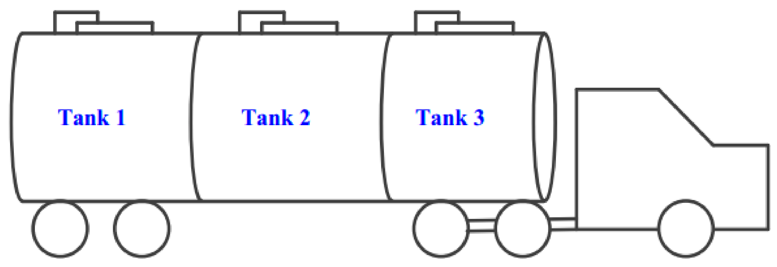
  There are 6 trucks available to use in each time zone. The trucks have capacities of 12, 12, 9, 9, 6 and 6 respectively. Each truck is divided into 3 equal compartments.

  (3.4)

  All customers must be visited.

The assigning and route constructing step is explained in the following example. The order of the raw milk farm obtained from Figure 3 is 3, 6, 4, 1, 2, 5 and 7. In

Table 2. The amount of raw milk in the raw milk farm i.

Raw Milk Farm	1	2	3	4	5	6	7
Raw milk (Ton)	4.1	5.6	2.4	4.5	3.5	5.6	5.8

, the available raw milk produced from each farm is shown. The distance between the factory (0) to the farms and from the farms to the farms is shown in

Table 3. The distance from raw milk farm i to j.

From/To	0	1	2	3	4	5	6	7
0	0	54.4	54.88	23.91	62.64	15.46	14.06	47.18
1	54.4	0	72.06	46.45	45.55	22.87	48.42	58.1
2	54.88	72.06	0	82.4	77.37	32.01	37.45	65.44
3	23.91	46.45	82.4	0	85.08	11.63	14.84	15.54
4	62.64	45.55	77.37	85.08	0	28.12	15.88	86.63
5	15.46	22.87	32.01	11.63	28.12	0	69.76	75.63
6	14.06	48.42	37.45	14.84	15.88	69.76	0	27.52
7	47.18	58.1	65.44	15.54	86.63	75.63	27.52	0

. The distance will be converted to the time used to travel within that connection by using an average speed of 60 km per hour. The order of the trucks is randomly generated, and it is 1, 6, 4, 5, 2 and 3. All parameters involved in the example are shown in

Table 4. Parameter setting of test instances.

Maximum capacity of raw milk tank	17 ton
Waiting cost of the truck before it can load	90 bath/hours
Cleaning cost of the raw milk tank of the factory	2000 bath
Capacity of compartment c in truck t	A compartment 4,3,2 ton
Cleaning cost of raw milk compartment c of truck t	400,300,200 bath/compartment
Fuel consumption rate of truck	4.5,4.2,3.9 bath/km
Time windows z	8 h
Loading time of raw milk to truck	10 ton/hours
Loading time of raw milk to Tank	10 ton/hours

Note: Approximately 33 Baht is one US dollar.

.

From

Table 5. The results of decoding vector 1 using the new decoding method.

Truck (Ton)/Time Zone	Route Sequence	Operating Time	Remaining Time of the Route	Distance (km)	Total Traveling Cost (Baht)	Cleaning of Compartment Cost (Baht)	Cleaning of Tanks Cost (Baht)	Total Cost (Baht)
12/1	0-3-6-4-1-0	298.58	181.42	154.58	695.61	1200	4000	1895.61
6/1	0-1-0	164	17.42	108.8	424.32	600		1024.32
9/2	0-2-5-0	210.35	269.65	102.35	429.87	900		1329.87
6/2	0-5-7-0	101.72	167.93	30.92	120.59	600		720.59
Total					1670.39	3300	4000	8970.39

, time zone no.1, truck no.1 travels from the factory to the raw milk collection center. A truck of 12 tons arrives at the collecting center at no.3, 6, 4 and 1, total travel time being 154.58 min. When the truck gets raw milk to a full capacity of 12 tons, it returns to the raw milk factory to transfer the raw milk to the storage tank. The time used to transfer raw milk and to leave is 144 min. The total time used is 298.58 min. Truck no.2 of six tons travels to raw milk center no.1 to service the remaining raw milk and then returns to the raw milk factory. The travel time is 108.8 min. The transfer of raw milk in and out takes 55.2 min. The total time used is 164 min. The remaining time is 17.42 min. This mechanism will be used to construct the route for all farms.

4.2. Mutation

The mutation process is the process where the mutant vector is constructed using three randomly target vectors ($X_{i,j,G}).$ Equation (37) is used to execute this process given F is the predefined scaling factor, where $V_{i,j,G+1}$ means mutant vector and $X_{r1,j,,G}$ $X_{r2,j,G}$, $X_{r3,j,G}$ means random target vector.

$$V_{i,G+1}= X_{r1,G}+F\left(X_{r2,G}-X_{r3,G}\right)$$

(37)

4.3. Recombination

The recombination process is the process where the trial vector is generated. Equation (38) is used to construct the trial vector ($U_{i,j,G}$) i position j iteration G where $X_{i,j,G}$ is the target vector i at position j in iteration G and $V_{i,j,G}$ is the trial vector i at position j in iteration G.

$$U_{i,j,G}=\{\begin{array}{c}{V}_{i,j,G+1} if ran{d}_{j,i} \le CR or j= I_{rand}\\ X_{j,i,G} if ran{d}_{j,i} > CR and j\ne I_{rand}\end{array}$$

(38)

After the recombination process, a trial vector will produce once more a second order trial vector (2rd-Tr). The 2rd-Tr will be generated from one out of three methods which are (1) the vector transition process, (2) the vector exchange process and (3) the vector insertion process.

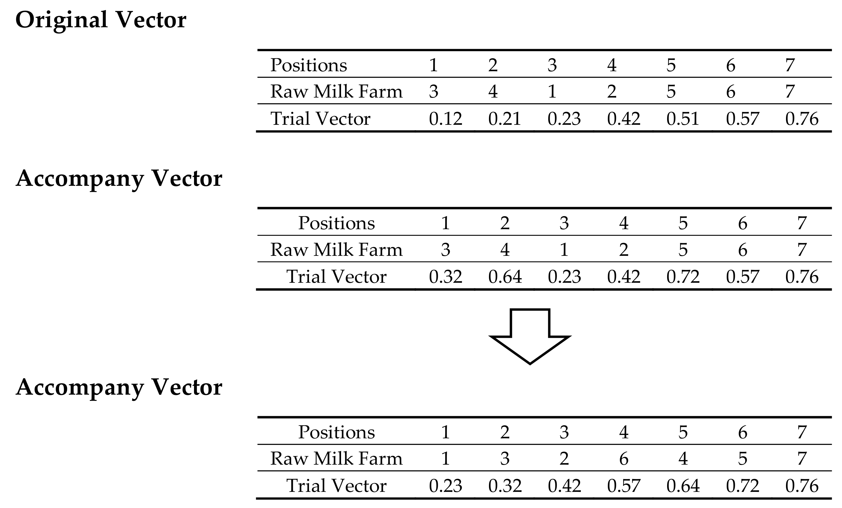
4.3.1. Vector Transition Process

This process starts from an integer number randomly laying from 1 to D where D is the number of positions in the vector; let us call this number the number of transition points (NT). Then randomly select the NT positions within D positions. Finally, the selected positions randomly generate a new value in the position. Figure 4 shows the vector transition process. The positions 1, 2 and 5 are selected as the transition points (the pre-selected number of the transition points is 3). The values in positions 1, 2 and 5 will be randomly generated while other position values remains unchanged.

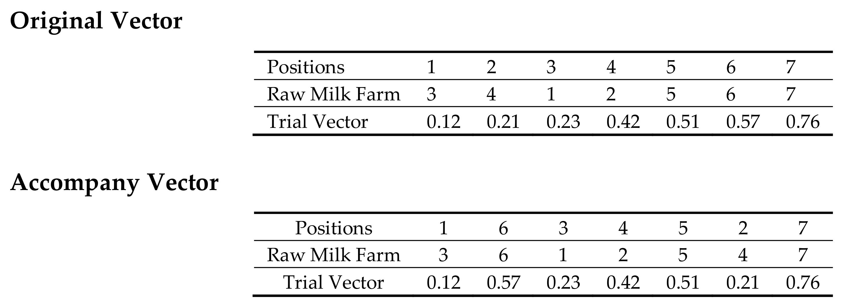
4.3.2. Vector Exchange Process

The vector exchange process is comprised of two steps, which are (1) the random selection of two exchange points in a trial vector and (2) the value exchange in selected positions. From Figure 5, the selected exchange points are 2 and 6. The value in the position 2 (0.21) is exchanged with the value in the position 6 (0.57). Thus, the new value in the position 2 is 0.57, and the new value in the position 6 is 0.21.

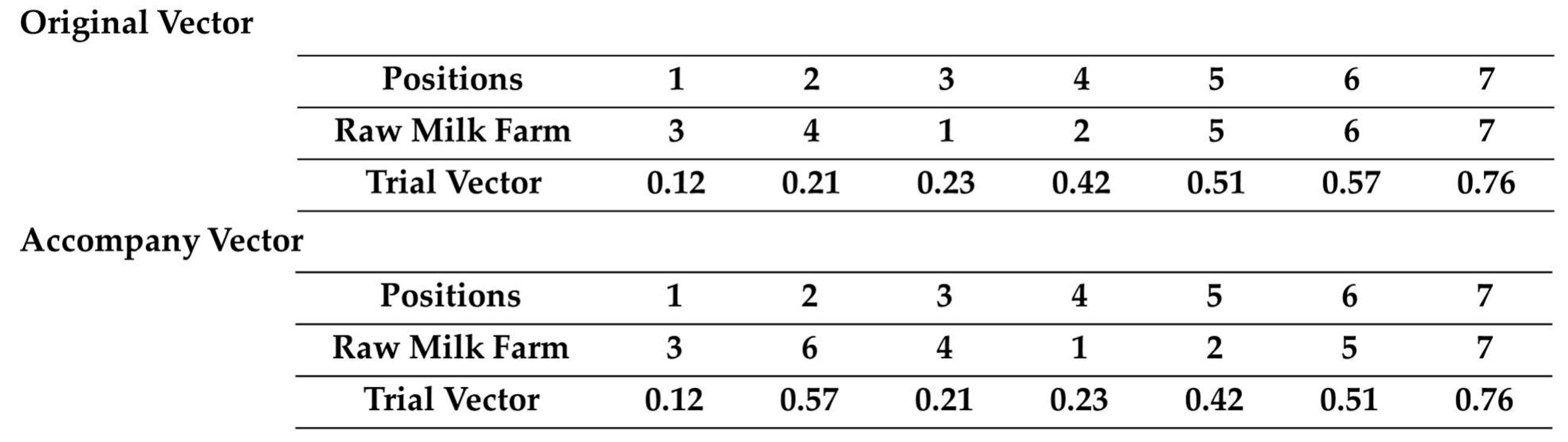
4.3.3. Vector Insertion Process

The vector insertion process starts from randomly selecting one insertion point and one moving point. Then the value from the moving point to the insertion point is inserted. All values after the insertion point will move backward. Figure 6 shows that position 3 is selected to be the insertion point and position 6 is selected to be the moving point. The value in position 6 (0.57) will be inserted into position 2. Thus, the values in positions 2, 3, 4, 5, and 6 are changed from 0.21, 0.23, 0.42, 0.51 and 0.57 to 0.57, 0.21, 0.23, 0.42 and 0.51, respectively.

The first trial vector and the 2rd-Tr will be decoded using the procedure which was explained in Section 4.1. The vector that has the lower cost among the first and the second trial vector will be used as the representative of the trial vector which will be used in the selection process.

4.4. Selection

The best selection chromosome process is used in this part of the procedure. A choice from the Target Vector and Trial Vector is made. The better vector between the two chromosomes is chosen as the new target vector to be uses as a starting vector in the next round.

$$X_{i,j,G+1}=\{\begin{array}{cc}{U}_{i,j,G}& if f\left(U_{i,j,G}\right)\le f\left(X_{i,j,G}\right)\\ U_{i,j,G}& if f\left(U_{i,j,G}\right)\ge f\left(X_{i,j,G}\right)\\ X_{i,j,G}& otherwise\end{array} and R_i\le P_i$$

(39)

where R_i is random number that is generated for trial vector i and P_i is calculated using Equation (40).

$$P_i= ex{p}^{-\frac{f\left(U_{i,j,G}\right)- f\left(X_{i,j,G}\right)}{MaxG-\left(G+1\right)\times K}}$$

(40)

where K is set to 3, T is G (iteration number), and MaxG is the predefined maximum number of iterations in the simulation. Equations (39) and (40) allow the DE mechanism to accept the worse solution due to the probability function which depend on the solution quality and the number of iterations which are used to let DE escape from the local optimal.

5. Computational Framework and Result

The proposed heuristics have been tested with 15 randomly generated test scenarios in which the number of farms was varied from 5 to 40. In addition, there was one case study which had the number of farms as 45. The randomly generated data was performed on a basis of the numbers in the case study. There are three local search techniques which are available to use which are the vector insertion, transition and exchange techniques. We present one new rule of the selection process. Therefore, eight proposed heuristics have been formed as shown in

Table 6. A list of the proposed heuristics.

DE-1	Original Differential Evolution
DE-2	Original Differential evolution and vector transition process
DE-3	Original Differential evolution and vector exchange process
DE-4	Original Differential evolution and vector insertion process
DE-5	Modified Differential evolution algorithm (Original DE and Disturb Selection)
DE-6	Modified Differential evolution algorithm and vector transition process
DE-7	Modified Differential evolution algorithm and vector exchange process
DE-8	Modified Differential evolution algorithm and vector insertion process

. The scaling factor F and crossover probability CR have been set to 0.5 and 0.8, respectively. The computational result is shown in

Table 7. The computational results of the total cost and the number of vehicles used for each instance.

Instance No.	# Of Clients	Lower Bound (BAHT)	% Diff
			DE-1	DE-2	DE-3	DE-4	DE-5	DE-6	DE-7	DE-8
1	5	6,012.70	0.00	0.00	0.00	0.00	0.00	0.00	0.00	0.00
2	10	10239.4	11.84	9.71	9.30	12.23	4.25	3.81	6.16	2.67
3	15	15161.1	12.59	10.60	11.87	8.93	4.07	0.29	0.48	2.04
4	15	15830.5	9.71	10.70	6.90	8.24	6.88	2.84	0.71	1.87
5	20	20566.1	10.80	6.26	5.69	10.14	3.34	3.38	2.67	2.99
6	20	20539.7	12.50	8.49	10.45	10.68	4.87	3.31	6.26	2.90
7	25	26407.1	10.85	11.63	10.04	11.68	3.86	3.48	3.59	2.96
8	25	27737.1	6.02	2.72	4.92	3.01	1.78	2.09	1.40	1.69
9	30	32618.5	8.29	6.26	4.88	7.65	3.67	3.12	3.25	2.36
10	30	32045.6	12.71	9.34	5.38	7.66	2.81	3.94	1.75	4.67
11	35	38076.0	8.29	10.16	5.91	5.55	5.47	1.73	5.30	2.89
12	35	37517.6	8.90	8.04	8.86	10.67	4.62	5.72	4.12	2.96
13	40	43807.1	6.72	6.61	5.07	4.70	3.59	3.11	2.77	3.47
14	40	40773.2	0.99	2.45	2.38	0.55	9.54	7.62	2.00	9.38
15	45	65931.3	4.50	3.75	3.38	3.27	1.49	0.48	0.94	0.60
16	45	65728.4	5.20	4.61	4.45	2.17	1.33	1.46	1.10	0.58
average			8.12	6.96	6.22	6.70	3.85	2.90	2.66	2.75

. All 8 algorithm (DE-1 to DE-8) has been executed using the number of iterations as the stopping criteria. The maximum number of iterations is set to 1000 iteration. Five simulations have been executed, and the best solution among the solutions which are generated within 5 runs is shown in Table 7. The results of DE-1 to DE-8 have been compared with the lower bound generated by Lingo using a 480 h computational time. The lower bound has units as Baht (cost), and the result shown in Table 7 of DE-1 to DE-8 is the percent difference which is calculated from Equation (41).

$$\%diff= \frac{Z_{DE}-Z_L}{Z_{DE}}\times 100\%$$

(41)

where % diff is the percent difference between the result of DE (Z_DE) is higher and the result of the lower bound (Z_L) found within 480 h.

The result shown in Table 7, using the real cost generated from each DE’s algorithm, was proved by applying the Wilcoxon Signed-Rank Test with a significant level 0.05 to discover if each of the methods were statistically different, and the statistics tested are shown in

Table 8. The Wilcoxon Signed-Rank Test on the total costs (p-value).

	DE-2	DE-3	DE-4	DE-5	DE-6	DE-7	DE-8
DE-1	0.034	0.009	0.012	0.009	0.007	0.008	0.009
DE-2	-	0.568	0.952	0.041	0.030	0.002	0.026
DE-3		-	0.818	0.012	0.009	0.0006	0.009
DE-4			-	0.03	0.019	0.003	0.014
DE-5				-	0.035	0.010	0.005
DE-6					-	0.192	0.912
DE-7						-	0.652

.

From Table 8, the total costs in all sizes were tested to find the difference between DE-1 to DE-8. The p-values of the DE-2, DE-3 and DE-4 algorithm methods’ significant levels are compared with DE-1 (original). The p-values of DE-2, DE-3 and DE-4 were at a significant level when compared with the DE-5, DE-6, DE-7 and DE-8 algorithm methods. In addition, the p-value of DE-5 was significant when compared with DE-6, DE-7 and DE-8. The improvement in DE is a suitable and highly effective method for solving a lot of attractions and complexes which are very hard for the vehicle routing of the tour transportation design problems.

Figure 7 shows the average percent difference of the DE’s algorithms without the selection process modification (DE-1 to DE-4) and the DE’s algorithms with the new selection process (using Equations (39) and (40)). The average percent difference of the original selection process is 7% while DE with the new selection process is 3.04% which is a 120% difference. This means that the new selection process improved the performance of the original selection process.

Figure 8 shows the average percent difference from the lower bound of the set of algorithms that uses different recombination processes. The result shows that the exchange process is the process that generates the best solution compared among all the new recombination processes.

In the next experiment, we will find the advantages and disadvantages of all the proposed algorithms. The case study has been used to execute this experiment. The stopping criteria has been set to 1, 5, 10, 20, 30, 40, 50 and 60 min. All algorithms have been executed 5 times, and the best solution among 5 solutions generated from each algorithm has been reported. The number reported in

Table 9. The % diff of DE-1 to DE-8 compared with the best solution generated by one out of DE-1 to DE-8.

Time/Min	ZMIN	% Diff
		DE-1	DE-2	DE-3	DE-4	DE-5	DE-6	DE-7	DE-8
5	66653.4	4.02	3.38	3.20	0.80	0.87	0.46	0.02	0.00
10	66640.4	4.04	3.40	3.23	0.82	0.89	0.48	0.00	0.02
20	66615.6	4.08	3.44	3.26	0.86	0.00	0.52	0.04	0.02
30	66572.9	4.15	3.50	3.33	0.92	0.06	0.32	0.00	0.08
40	61486.3	12.77	12.06	11.88	9.27	4.34	4.62	0.00	3.53
50	60164.1	15.24	14.53	14.34	11.68	6.72	5.86	0.00	4.89
60	59767.42	16.01	15.29	15.10	12.42	7.46	6.60	0.00	5.62
average		8.62	7.94	7.76	5.25	2.91	2.69	0.01	2.02

is the GAP between the minimum costs generated among 8 proposed algorithms using Equation (42).

$$\%diff= \frac{Z_{DE}-Z_{Min}}{Z_{Min}}\times 100\%$$

(42)

where % diff is the percent difference between the results of DE-1 to DE-8 (Z_DE) and the minimum cost when comparing the result of all the DEs. For example, if DE-1 to DE-8 generates costs of 66,653.4, 66,640.4, 66,615.6, 66,572.9, 66,824.2, 61,486.9, 61,476.1 and 66,692.2 respectively, the Z_MIN is 61,476.1, which is the solution of DE-7.

From Table 9, we can see that when the computational result is higher, the MDE (DE-5 to DE-8) outperforms the original DE. All the best solutions among the 8 proposed heuristics (GAP = 0.00) are always one out of 4 members of MDE in all computational times used. When the computational result is higher, the DE performs worse than when the computational time is short while the MDE performs better when the computational time is higher. To prove that, we plot graph of all 8 algorithms while it executes the first iteration to the last iteration to see how it is behaved while searching for the result, and the result is shown in Figure 9.

From Figure 9, we can see that the original DE algorithm converts very fast and gets stuck in the local optimal and that the best result remains unchanged until the simulation is terminated. The MDE performs differently; it still finds a better solution, and the best solution which is reported is often changed and continues searching. Figure 9 shows that the MDE clearly outperforms the original version of DE.

6. Conclusions

The objective of this research was to minimize the total transportation cost and the truck’s cleaning cost in an optimization problem within the dairy industry. The transportation cost directly depends on the fuel usage. The fuel usage occurs during the transportation of the truck and the waiting time when it arrives at the factory and cannot transfer the raw milk into the production tank. The proposed work has several strengths over the original VRP problems, which was the first major contribution of this work. These strengths come from its ability to incorporate the following aspects into the model: (1) one heterogeneous fleet with multiple compartments is being used; (2) one compartment can mix the raw milk from at most two farms to maintain to quality of the milk; (3) the truck must arrive at the farms within the time window of the farms; (4) the waiting time of the truck while it is waiting to load the milk into the production line is considered as the cost term; (5) the truck is allowed to collect raw milk more than one time per day; and (6) the start time of the truck affects the total cost.

Moreover, this article improves the original DE by modifying three steps of the DE which are (1) presenting the effective decoding method, (2) using 3 different local search techniques and (3) presenting a new rule of the selection process. Subsequently, we have shown how this comprehensive model may be used practically, paving way for future researchers to use our model for similar optimization processes.

The other major finding of this work was the comparisons made between various differential evolution algorithms (DEs). The modification of the selection process significantly improved the efficiency of the original DE. From Figure 7, we can see that the MDE reduces more than 120% of the cost compared with the original DE. The new selection process allowed the proposed algorithm to accept the worse quality solution. This gives the algorithm more chances to escape from the local optimal. Moreover, the modification of the recombination process outperforms the original version of DE. From Figure 8, the original DE has the GAP from the lower bound 5.98% while the modification of recombination process has the GAP from 4.44 to 4.93%. This is because of the new recombination process enhancing the intensification search of the original DE. Therefore, the better solution is easier to obtain. From Figure 7 and Figure 8, it is clear that both the modification of the recombination and selection processes we proposed in this article, originally from our research, outperform the original version of DE.

We designed the algorithm to reflex the mathematical model shown in Section 3 where all the variables can be discovered. From the experience of the simulation, we found that the result of the solution obtained from the proposed problem using DE to solve some behaviours differed from that of the original VRP such as (1) generally in VRP, the vehicle always will start the route when the it is ready, but in our study the vehicle sometimes waits in the depot so that it has no waiting time to load the milk into the production tank when it finishes collecting the raw milk from all farms; (2) the model tries to use as few vehicles as possible to reduce the cleaning cost, but this attribute also depends on the cleaning cost; (3) some farms are not selected to be visited after another farm even if it is very close to the current farm due to it having a high amount of milk which makes the vehicle not have enough time to go back to the production line in time when the production tank is ready so that it can reduce the cost generated from the waiting time of the vehicle.

Finally, we can conclude that the original DE performs worse while using long computational time and that the MDE performs better while the computational time is longer. The MDE increases the possibility to find the new best solution (see Figure 9) due to MDE being able to escape from the optimal solution caused by the new selection method that we introduce in this article.

The milk storing cost during the waiting time of the truck while another truck is loaded can be dramatically reduced if the milk producer adds more production tanks. If it is so, the mathematical model has to be changed which will affect the design of the algorithm and must be slightly improved. The more sophisticated algorithm can be developed using a hybrid or combination of the metaheuristics, such as adaptive large scale neighbourhood search, large scale neighbourhood search and variable neighbourhood search.

References

1. Lambert, J.C. Global lactoperoxidase programme: the lactoperoxidase system of milk preservation. Bull. Int. Dairy. Fed. 2001, 365, 19–20. [Google Scholar]
2. Basnet, C.; Foulds, L.R.; Wilson, J.M. An exact algorithm for a milk tanker scheduling and sequencing problem. Ann. Oper. Res. 1999, 86, 559–568. [Google Scholar] [CrossRef]
3. Worasan, K.; Sethanan, K.; Chaikanha, N. Dairy transportation problem with no mixing of raw milk and time windows constraints. In Proceedings of the APIEMS 2014, Jeju, Korea, 12–15 October 2014. [Google Scholar]
4. Sethanan, K.; Pitakaso, R. Differential Evolution Algorithms for Scheduling Raw Milk Transportation. Comput. Electron. Agric. 2016, 121, 245–259. [Google Scholar] [CrossRef]
5. De, A.; Awasthi, A.; Tiwari, M.K. Robust Formulation for Optimizing Sustainable Ship Routing and Scheduling Problem. IFAC-PapersOnLine 2015, 48, 368–373. [Google Scholar] [CrossRef]
6. De, A.; Vamsee, K.R.M.; Angappa, G.; Nachiappan, S.; Tiwari, M.K. Composite particle algorithm for sustainable integrated dynamic ship routing and scheduling optimization. Comput. Ind. Eng. 2016, 96, 201–215. [Google Scholar] [CrossRef]
7. Dominguez, O.; Guimarans, D.; Juan, A.A.; Nuez, I. A Biased-Randomised Large Neighbourhood Search for the two-dimensional Vehicle Routing Problem with Backhauls. EJOR 2016, 255, 442–462. [Google Scholar] [CrossRef]
8. Can, B.K.; Can, K. An ant colony system empowered variable neighbourhood search algorithm for the vehicle routing problem with simultaneous pickup and delivery. Expert Syst. Appl. 2016, 66, 163–175. [Google Scholar] [CrossRef]
9. De, A.; Kumar, S.K.; Angappa, G.; Manoj, K.M. Sustainable maritime inventory routing problem with time window constraints. EAAI 2017, 61, 77–95. [Google Scholar] [CrossRef]
10. De, A.; Choudhary, A.; Tiwari, M.K. Multiobjective Approach for Sustainable Ship Routing and Scheduling With Draft Restrictions. IEEE T. Eng Manag. 2019, 66, 35–51. [Google Scholar] [CrossRef]
11. De, A.; Pratap, S.; Kumar, A.; Tiwari, M.K. A hybrid dynamic berth allocation planning problem with fuel costs considerations for container terminal port using chemical reaction optimization approach. Ann. Oper. Res. 2018, 1–29. [Google Scholar] [CrossRef]
12. Caramia, M.; Guerriero, F. A heuristic approach for the truck and trailer routing problem. J. Oper. Res. Soc. 2010, 61, 1168–1180. [Google Scholar] [CrossRef]
13. Caramia, M.; Guerriero, F. A milk collection problem with incompatibility constraints. Interfaces. 2010, 40, 130–143. [Google Scholar] [CrossRef]
14. Fisher, M.L.; Jaikumar, R. A generalized assignment heuristic for vehicle routing. Networks 1981, 11, 109–124. [Google Scholar] [CrossRef]
15. Chao, I.M. A tabu search method for the truck and trailer routing problem. Comput. Oper. Res. 2002, 29, 33–51. [Google Scholar] [CrossRef]
16. Scheuerer, S. A tabu search heuristic for the truck and trailer routing problem. Comput. Oper. Res. 2006, 33, 894–909. [Google Scholar] [CrossRef]
17. Tan, K.C.; Chew, Y.H.; Lee, L.H. A hybrid multi-objective evolutionary algorithm for solving truck and trailer vehicle routing problems. Eur. J. Oper. Res. 2006, 172, 855–885. [Google Scholar] [CrossRef]
18. Hoff, A.; Løkketangen, A. A tabu search approach for milk collection in western Norway using trucks and trailers. In Proceedings of the Sixth Triennial Symposium Transportation Anal. TRISTAN VI, Phuket Island, Thailand, 10–15 June 2007. [Google Scholar]
19. El Fallahi, A.; Prins, C.; Wolfler Calvo, R. A memetic algorithm and a tabu search for the multi-compartment vehicle routing problem. Comput. Oper. Res. 2008, 35, 1725–1741. [Google Scholar] [CrossRef]
20. Storn, R.; Price, K. Differential evolution—a simple and efficient heuristic for global optimization over continuous spaces. J. Glob. Optim. 1997, 11, 341–359. [Google Scholar] [CrossRef]
21. Pitakaso, R. Differential Evolution algorithm for Simple Assembly Line Balancing. J. Ind. Prod. Eng. 2015, 32, 104–114. [Google Scholar]
22. Pitakaso, R.; Sethanan, K. Modified Differential Evolution algorithm for Simple Assembly Line Balancing with limit on number of machines. Eng. Optimiz. 2015, 48, 253–271. [Google Scholar] [CrossRef]
23. Liao, T.W.; Egbelu, P.J.; Chang, P.C. Two hybrid differential evolution algorithms for optimal inbound and outbound truck sequencing in cross docking operations. Appl. Soft Comput. 2012, 12, 3683–3697. [Google Scholar] [CrossRef]
24. Lai, M.Y.; Cao, E.B. An improved differential evolution algorithm for vehicle routing problem with simultaneous pickups and deliveries and time windows. Eng. Appl. Artif. Intell. 2010, 23, 188–195. [Google Scholar]
25. Hou, L.; Zhou, H.; Zhao, J. A novel discrete differential evolution algorithm for stochastic VRPSPD. J. Computat. Infor. Syst. 2010, 6, 2483–2491. [Google Scholar]
26. Dechampai, D.; Tanwanichkul, L.; Sethanan, K.; Pitakaso, R. A differential evolution algorithm for the capacitated VRP with flexibility of mixing pickup and delivery services and the maximum duration of a route in poultry industry. J. Intell. Manuf. 2015, 28, 1357–1376. [Google Scholar] [CrossRef]
27. Sethanan, K.; Pitakaso, R. Improved differential evolution algorithms for solving generalized assignment problem. Expert Syst. Appl. 2016, 45, 450–459. [Google Scholar] [CrossRef]
28. Akararungruangkul, R.; Kaewman, S. Modified Differential Evolution Algorithm Solving the Special Case of Location Routing Problem. Math. Comput. Appl. 2018, 23, 34. [Google Scholar] [CrossRef]
29. Chomchalao, C.; Kaewman, S.; Pitakaso, R.; Sethanan, K. An Algorithm to Manage Transportation Logistics That Considers Sabotage. Risk. Adm. Sci. 2018, 8, 39. [Google Scholar] [CrossRef]
30. Kaewman, S.; Akararungruangkul, R. Heuristics Algorithms for a Heterogeneous Fleets VRP with Excessive Demand for the Vehicle at the Pickup Points, and the Longest Traveling Time Constraint: A Case Study in Prasitsuksa Songkloe, Ubonratchathani Thailand. Logistics 2018, 2, 15. [Google Scholar] [CrossRef]
Figure 1. A milk vehicle with multi-compartments.
Agriengineering 01 00006 g001
Figure 2. An illustration of the tour representing a solution of the problem.
Agriengineering 01 00006 g002
Figure 3. An example of how to depict the order of the raw milk farm.
Agriengineering 01 00006 g003
Figure 4. Example of the vector transition process.
Agriengineering 01 00006 g004
Figure 5. Example of the vector exchange process.
Agriengineering 01 00006 g005
Figure 6. Example of the vector insertion process.
Agriengineering 01 00006 g006
Figure 7. The average percent difference from the lower bound of the set of algorithms (DE-1 to DE-4) used in the original selection process and the set of algorithms that use the new selection process.
Agriengineering 01 00006 g007
Figure 8. The average percent difference of the DE using different processes to generate the 2nd order of the trial vector.
Agriengineering 01 00006 g008
Figure 9. The best solution plots of the 8 proposed heuristics.
Agriengineering 01 00006 g009