Article

The Modelling of the Evapotranspiration Portion of the Water Footprint: A Global Sensitivity Analysis in the Brazilian Serra Gaúcha

by
Gustavo Mendes Platt
1,*,
Vinícius Kuczynski Nunes
1,
Paulo Roberto Martins
1,†,
Ricardo Gonçalves de Faria Corrêa
1 and
Francisco Bruno Souza Oliveira
2,*
1
Graduate Program in Agroindustrial Systems and Processes, School of Chemistry and Food, Federal University of Rio Grande (PPGSPA/FURG), Santo Antônio da Patrulha 95500-000, Brazil
2
Graduate Program in Computational Modelling in Science and Technology, Department of Engineering and Computing, State University of Santa Cruz (PPGMC/UESC), Ilhéus 45662-900, Brazil
*
Authors to whom correspondence should be addressed.
Current address: Graduate Program in Environmental Quality, Feevale University, Novo Hamburgo 93548-480, Brazil.
Earth 2024, 5(2), 133-148; https://doi.org/10.3390/earth5020007
Submission received: 20 March 2024 / Revised: 11 April 2024 / Accepted: 19 April 2024 / Published: 20 April 2024

Abstract

:
Water footprints have been widely used to illustrate the consumption of water in many situations, for instance, in products, processes, or regions of interest. In this work, we analyzed—using a sensitivity analysis approach—the effect of some variables in the calculation of the water footprint in the viticulture in the Brazilian Serra Gaúcha (the major producing region of Brazilian wine). The classical Penman–Monteith model for evapotransporation was considered, with uncertainties in some parameters (dead mulch covering a fraction of the vineyard, maximum temperatures for some months, the altitudes and latitudes of the site). A sensitivity analysis was conducted using the SAFE toolbox under Octave framework. The results indicated that the the portion of the water footprint corresponding to evapotranspiration is more sensitive to the values of the mulch-covered fraction and the altitude of the site in comparison with the latitude and the maximum temperatures.

1. Introduction

Water consumption in the viticulture is gaining more attention every year [1,2]. Thus, it is necessary to understand the factors that affect it and in which ones we can interfere to reduce water use. In recent decades, Brazil has been receiving attention for its capacity to produce wine [3]. Furthermore, the most traditional and main wine hub in Brazil is the Brazilian Serra Gaúcha [4,5,6].
A well-established measure of water consumption is called water footprint. The water footprint concept was introduced by Hoekstra and Hung [7] and represents the consumption of water by a crop, product, region, or nation (for instance). The water footprint is usually classified as green, blue, and gray water. In essence, green water indicates the portion of water arising from rain and snow, whereas blue water corresponds to the water coming from irrigation. Finally, the gray portion refers to the necessary quantity of water employed in dilution processes (in order to achieve the concentration of each pollutant in a river, for instance). In the wine industry, the study of the water footprint is fairly recent, with calculations presented for New Zealand, Italy, South Africa, and Portugal, for instance [8,9,10,11]. Water consumption in wineries and in vineyards must be considered. Water is consumed through evapotranspiration, irrigation, and the use of fertilizers and agrochemicals, among others [9].
An important part of the water footprint calculation of a crop is usually conducted considering the evapotranspiration concept. Evapotranspiration is a combined process of evaporation and transpiration by a crop. The initial step in the calculation of evapotranspiration is the determination of the reference evapotranspiration ( E T 0 ). The reference evapotranspiration is commonly calculated using the Penman–Monteith model [12], which is a well-established methodology. Using a small set of parameters (latitude, altitude, wind speed, temperatures of the site), this model permits the evaluation of the reference evapotranspiration E T 0 . The crop evapotranspiration ( E T c ) is calculated using the value of E T 0 and a crop coefficient, which considers the different growth stages of a particular crop and the existence of dead mulch (for instance) [12]. Clearly, the different quantities employed in the calculation of the E T 0 and E T c parameters are subject to uncertainty (for instance, temperatures and wind speeds), and the main objective of a sensitivity analysis (in this context) is to evaluate the effect of these uncertainties on the calculated values of evapotranspiration [13,14,15]. Furthermore, the productivity of the crop is also subject to uncertainty, which can have a direct impact on the calculation of the water footprint.

1.1. Previous Studies

Many studies deal with sensitivity analysis using the Penman–Monteith model for the reference evapotranspiration, considering different parameters and locations. Beven [16] studied the sources of errors and presented a sensitivity analysis study for the Penman–Monteith equation for three meteorological sites in England and Wales. The author observed a higher dependence of the vegetation type on the evapotranspiration, in comparison to climatic differences between the three sites analyzed. Ndiaye et al. [14] analyzed the effects of maximum/minimum temperatures, solar radiation, wind speed, and maximum/minimum relative humidity on evapotranspiration in different localities in Burkina Faso. Irmak et al. [17] conducted a sensitivity analysis study of several parameters (maximum/minimum wind speed, maximum/minimum air temperatures, vapor pressure deficit, and solar radiation) in some regions of the United States of America, concluding that E T 0 is more sensitive to variations in the vapor pressure deficit. Debnath et al. [18] conducted a sensitivity analysis study for the reference evapotranspiration value in India, indicating that E T 0 is more sensitive to solar radiation. Furthermore, Debnath et al. [18] noted a linear relationship between the value of E T 0 and the variables under consideration (maximum and minimum temperatures, solar radiation, relative humidity, and wind speed). Biazar et al. [19] conducted a sensitivity analysis study for the reference evapotranspiration E T 0 , using different models, in a humid region of Iran. The findings of Biazar et al. [19] indicate a high sensitivity of E T 0  to the maximum temperatures and number of sunshine hours, and some lower sensitivities with respect to the minimum temperature and wind speed. Arunrat et al. [20] analyzed the impact of climate change on the water footprint for rice, cassava, maize, soybean, and mung bean in Thailand. The authors considered changes in demography and economics, as well as the greenhouse effect, in the studied scenarios (Shared Socioeconomic Pathways—SSPs). Arunrat et al. [20] concluded that the water footprint for the studied crops in the future will be closely related to the yields, considering the greenhouse effect. Furthermore, some crops (maize, soybean, mung bean, and cassava) appear as alternatives to rice during the dry seasons. Rossi et al. [21] studied the water footprints for olive production in Italy (considering the green, blue, and gray portions of the water footprint). The authors observed a predominance of the green water footprint in comparison to the blue and gray portions. Furthermore, it was observed by Rossi et al. [21] that the water footprint was severely influenced by the productivity, even in some years with low precipitation, which is in agreement with the results of Arunrat et al. [20] (i.e., the effects of some parameters in the reference evapotranspiration can be compensated by an increase in the productivity, considering the calculation of the water footprint). Arunrat et al. [22] presented a study analyzing the nitrogen, carbon, and water footprints of organic and conventional rice in Thailand in the 2018–2021 period. The authors highlighted that the water footprint for the conventional crop is higher than the value for the organic rice (mainly with respect to the gray water footprint). Recently, Yong et al. [23] presented a review study concerning the different sensitivity analysis techniques applied in the calculation of the reference evapotransporation. The results obtained by Yong et al. [23] indicated that the global sensitivity analysis studies are recent and restricted to a few countries (Australia, Malaysia, the United States, and China). A recent work by Sabino and de Souza [24] presented a study of global sensitivity analysis for the Penman–Monteith model to calculate the reference evapotranspiration in the state of Mato Grosso, Brazil, using the Sobol’ method.
Specifically considering the calculation of the water footprint, Zhuo et al. [25] presented a study of uncertainty and sensitivity analysis in the water footprint for the production of maize, soybean, rice, and wheat in China (Yellow River Basin). Recently, Li et al. [26] conducted a sensitivity analysis study in the production of wheat, rice, maize, and soybean in China. In this study, the authors considered the value of the reference evapotranspiration E T 0 as one of the parameters.

1.2. Proposed Current Study

In this work, we propose a detailed sensitivity analysis procedure in the water footprint calculation for the viticulture in the Serra Gaúcha, Brazil, located in the Rio Grande do Sul state. As mentioned previously, the Serra Gaúcha is Brazil’s main wine-producing region. We consider, as parameters, the altitude and the latitude of the site (which impacts the reference evapotranspiration) and the existence of dead mulch in the vineyard (affecting the crop evapotranspiration). In addition to these, the maximum temperatures for the months of October, November, and December are also considered as parameters. Obviously, there is a huge scope for choosing other parameters for the sensitivity analysis (for instance, wind speed and humidity). On the other hand, the main focus of this work is to detail the influence of some parameters which can be objects of decision (for instance, the place to set up a vineyard and the use of a soil management technique in order to minimize the water consumption). Thus, the results of the water footprint sensitivity analysis provide supplementary data for decision-making purposes. Moreover, considering the rising temperatures in the Rio Grande do Sul state (Brazil) [27,28], the effects of maximum temperatures on the water footprint are also taken into account. Moreover, Biazar et al. [19] indicated that the most sensitive parameter for E T 0 in a humid region in Iran is the maximum temperature, which justifies this choice. It should be noted that this study only covers the portion of the water footprint that refers to crop evapotranspirationin the vineyard. One must also bear in mind that the aim of this study is not to present comparisons between evapotranspiration models, despite the importance of such studies (see, for instance, [29,30,31,32]).
Although the analysis is specific to a particular region, the procedures used are applicable to any location worldwide. Here, we employ the SAFE toolbox (under Octave [33]) for sensitivity analysis developed by Pianosi et al. [34]. Global sensitivity analysis tools are also available on other platforms; see, for instance, Borges et al. [35]. Finally, it should be emphasized that the use of global sensitivity analysis techniques in water footprint calculations has not been frequently found in the literature.
The main innovation of this work is to combine global sensitivity analysis techniques with evapotranspiration models in order to verify the effect of geographical and climatic parameters on the water footprint, with the aim of informing decision-making. In addition to pointing out the direction of the effects of changes in each of the variables under study, our sensitivity analysis study will be employed to indicate possible offsetting effects between the input parameters of the model.

2. Materials and Methods

2.1. Modelling

In this section, the mathematical models under consideration are detailed, namely the reference evapotransporation model (Penman–Monteith model) ( E T 0 ), the crop evapotranspiration model ( E T c ), and the water footprint model ( W F ).

2.1.1. The Reference Evapotranspiration Model

The reference evapotranspiration ( E T 0 , in mm/day or mm/month, depending on the time step employed) was represented by the Penman–Monteith model [12]:
E T 0 = 0.408 Δ ( R n G ) + γ p 900 T + 273 u 2 ( e s 0 e a ) Δ + γ p ( 1 + 0.34 u 2 ) ,
where R n is the net flux in solar radiation (MJ/ m 2 /day), G is the heat flux in the soil (MJ/ m 2 /day), T is the mean air temperature at 2 m height (°C), e s 0 is the saturation vapor pressure (kPa), e a is the actual vapor pressure (kPa), Δ is the slope of the vapor pressure curve, γ p is the psychrometric constant (kPa/K), and u 2 is the wind speed at 2 m (m/s).
In order to clarify the objectives of the sensitivity analysis study, the main terms of Equation (1) must be detailed. Even though this equation is well known, a detailed analysis of the model permits a clear understanding of the nonlinearities of the equations involved in the problem. Therefore, the calculations of e s 0 , Δ , γ p , R n , and G will be explained in detail, as well as the correlated quantities. A detailed description of these parameters is presented in the Appendix A.
The Penman–Monteith equation was chosen due to the large number of scientific studies involving this model.

2.1.2. Crop Evapotranspiration Model

The crop evapotranspiration can be obtained using the value of the reference evapotranspiration, considering the different development stages of the crop, according to [12]:
E T c = E T 0 K c ,
where K c is the crop coefficient. Usually, three different stages are considered (initial, mid-season, and late season stages), with three values for K c . The FAO [12] recommendation for grape wines are K c i n i t = 0.30 , K c m i d = 0.70 , and K c l a t e = 0.45 , where the subscripts init, mid, and late refer, respectively, to the initial, mid, and late stages of the development of the crop. On the other hand, some parameters can affect the values of K c , such as the existence of dead mulch [36]. According to Fonseca [37], the effect of dead mulch in the value of K c i n i t can be represented by the following expression:
K c i n i t , d c = K c i n i t 1 0.50 f d m ,
where f d m is the dead mulch coverage fraction. K c i n i t , d c represents the crop coefficient considering the existence of dead mulch. Thus, an obvious effect of the use of dead mulch is the reduction in the values of the crop evapotranspiration ( E T c ). It must be emphasized that the use of mulch is a common practice in the Brazilian Serra Gaúcha, as pointed out by Rosa et al. [38], which justifies the study of the impact of this parameter on the water footprint. The use of organic mulching in vineyards to reduce E T c was also reported by López-Urrea et al. [39]. Furthermore, Fonseca [37] pointed out that although the use of mulch is very common for wine production in the tropical regions of Brazil, this practice has also been observed in temperate regions.

2.1.3. Water Footprint Model

In this work, it was assumed that the water demand by the crop was fully met. Thus, the water footprint can be calculated as [7]
W F = 10 × E T c Y ,
where Y is the grape productivity by hectare (ton/ha) and E T c is in mm/month. The factor 10 converts the evapotranspiration into m 3 /ha. The sum refers to the months of the year. We are not differing between the types of water footprint (green and blue).

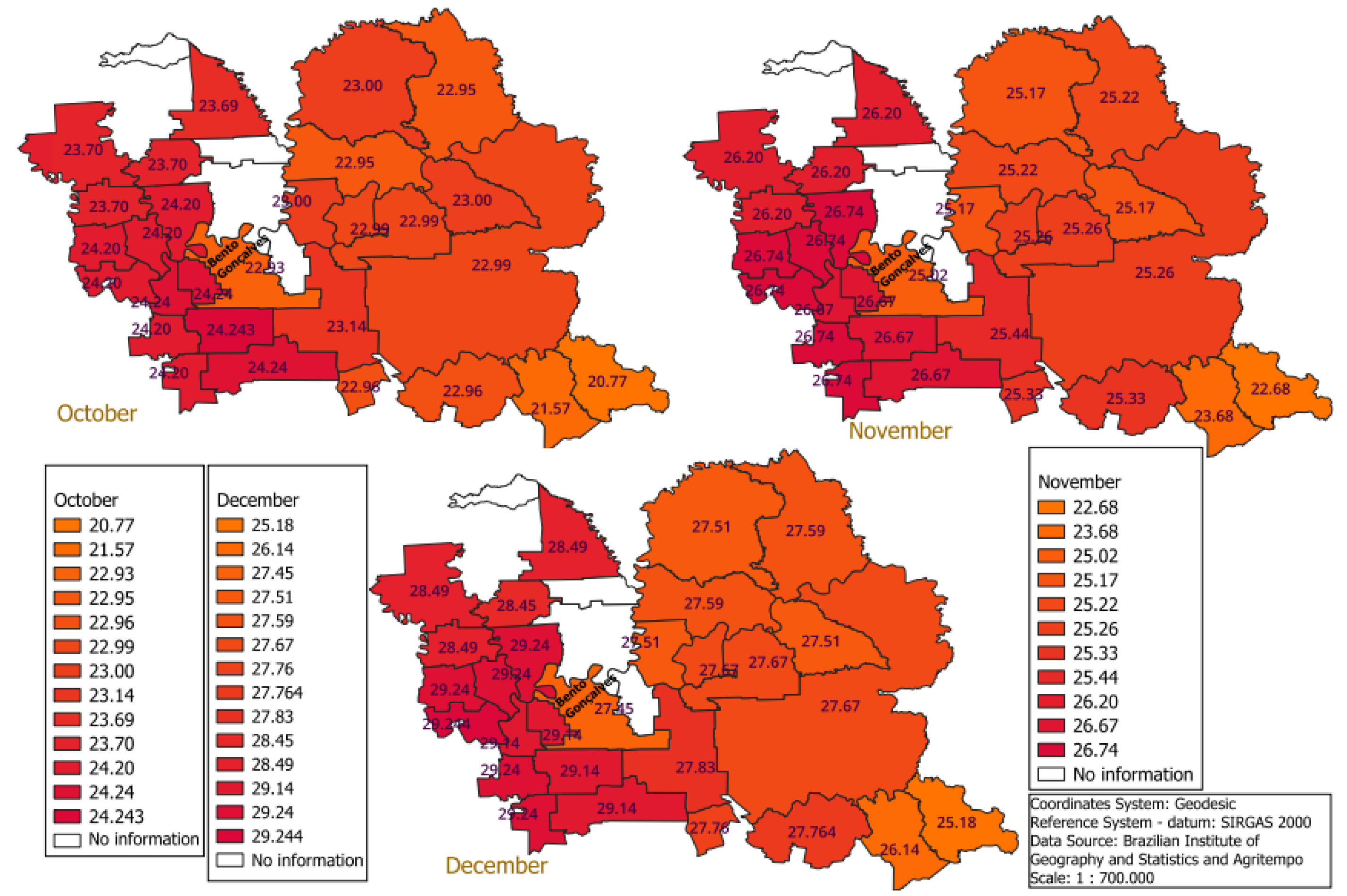
2.2. Brazilian Serra Gaúcha

We considered the latitudes between the cities of Nova Araçá (−28.654549°) and Gramado (−29.433653°). Figure 1 presents an altimetric map of the Rio Grande do Sul state, in Brazil, as well as the localization of the Serra Gaúcha, the region under study. The main objective of these maps is to detail the ranges of latitudes and longitudes for the sensitivity analysis. In the Serra Gaúcha, the elevations are in the range from 206 m to 926 m (considering the existence of valleys in the region). In recent years, there has been an increase in the production of wine at altitudes above 700 m (for example, the so-called Altos de Pinto Bandeira wine). Furthermore, the soil management techniques in vineyards usually employ mulching practices [40]. With respect to the dead-mulch-covered fraction, f d m , this parameter is in the interval 0 , 1 .
Calculations were conducted using information from the municipality of Bento Gonçalves, Brazil, the main wine-producing city in the Serra Gaúcha. Data for temperatures, relative humidities, and number of hours of sunlight per day were obtained from Climate Data (Available online: https://pt.climate-data.org/america-do-sul/brasil/rio-grande-do-sul/bento-goncalves-1386/, accessed on 9 April 2024). Wind velocities were obtained from Weather Spark (Available online: https://pt.weatherspark.com/y/29709/Clima-caracter%C3%ADstico-em-Bento-Gon%C3%A7alves-Brasil-durante-o-ano, accessed on 9 April 2024). We considered variations of 3 °C in the maximum temperatures of the months of October, November, and December (an arbitrary choice in order to evaluate the effect of the maximum temperatures on the water footprint). These variations are far greater than the differences of the maximum temperatures in the region under study (even considering the differences in altitude and latitude). In order to subsidize the choice of this temperature range, Figure 2 presents the maximum temperatures in the Serra Gaúcha for October, November, and December in the last decade (2013–2023). We can observe that the maximum temperatures for these months are in the interval T b a s e ± 3 °C, where T b a s e refers to the temperature in the city of Bento Gonçalves.
A medium productivity value Y for grape production was assumed, Y = 10 ton/ha. Usually, three scenarios may be considered for grape production in the Serra Gaúcha: Y m a x = 12 ton/ha, Y a v g = 10 ton/ha, and Y m i n = 8 ton/ha [41] (obviously, the effect of the productivity exhibits a direct effect on the water footprint, and a sensitivity analysis is not necessary for this variable). Furthermore, we used a typical conversion factor of 70% to calculate the number of liters of wine by ton of grape, i.e., a ton of grapes is capable of producing 700 L of wine.

2.3. Global Sensitivity Analysis Techniques

As mentioned previously, we employed the SAFE package [34,42], under Octave, to perform the sensitivity analysis. Here, some of the steps proposed by Noacco et al. [42] in conducting the sensitivity analysis were taken.

2.3.1. Sampling Strategy

The most popular sampling strategy is Latin Hypercube Sampling (LHS) [43]. Some recent works employed LHS in sensitivity analysis studies dealing with evapotranspiration calculations [44,45,46]. Considering that each coordinate of a vector is in the interval [ 0 , 1 ] , a Latin Hypercube Sample with N intervals shows a random distribution of N values, with one value in each of the intervals 0 , 1 N , 1 N , 2 N , , 1 1 N , 1 . In practice, the Latin Hypercube strategy has been optimized, for instance, with random permutations of the values (coordinate exchange) and with a maximization of the minimum distance between sample points (called the maximin criterion), as implemented in the SAFE toolbox [34]. The sampling strategy employed here was Latin Hypercube Sampling [47,48], with N = 3000 .
A simple substitution of the Latin Hypercube Sample in the model (in our work, the calculation of the water footprint in the wine viticulture) permitted us to obtain the responses of the model using, for instance, scatter plots.

2.3.2. Analysis of Elementary Effects (EEs)

The first global sensitivity analysis technique applied in our computational experiments was the analysis of the elementary effects (EEs). As pointed out by Morris [49], the main objective of the analysis of elementary effects (also called the Morris method [49]) is to determine whether an effect of such a variable on the response of the model is (i) negligible, (ii) linear and additive, (iii) nonlinear, or (iv) involved in interactions with other variables.
An elementary effect E E i for an input i is defined by the following [49]:
E E i ( X ) = ( y ( X 1 , , X i 1 , X i + Δ X , X i + 1 , , X k ) y ( X ) ) Δ X ,
where X is the vector representing the variables of the problem and Δ X is a perturbation in the vector X (only in the position i). Each value of X i may vary in some levels. We aim to compute r EEs, using r trajectories [50]. The mean of the effects for r trajectories is then calculated by [50]
μ i = 1 r i = 1 r E E i .
The standard deviation is represented by [50]
σ i = i = 1 r E E i μ i 2 r ,
In our computations, we computed 500 elementary effects ( r = 500 ). A bootstraping approach (i.e., a resampling strategy) was also applied [51], with N b o o t = 100 . Furthermore, the SAFE package employed the “revised version” of μ , represented by μ * (using the absolute values of the elementary effects) [52]. Considering r elementary effects, the number of evaluations of the model is n = r ( M + 1 ) = 500 ( 6 + 1 ) = 3500 , where M is the number of variables considered in the analysis [53].

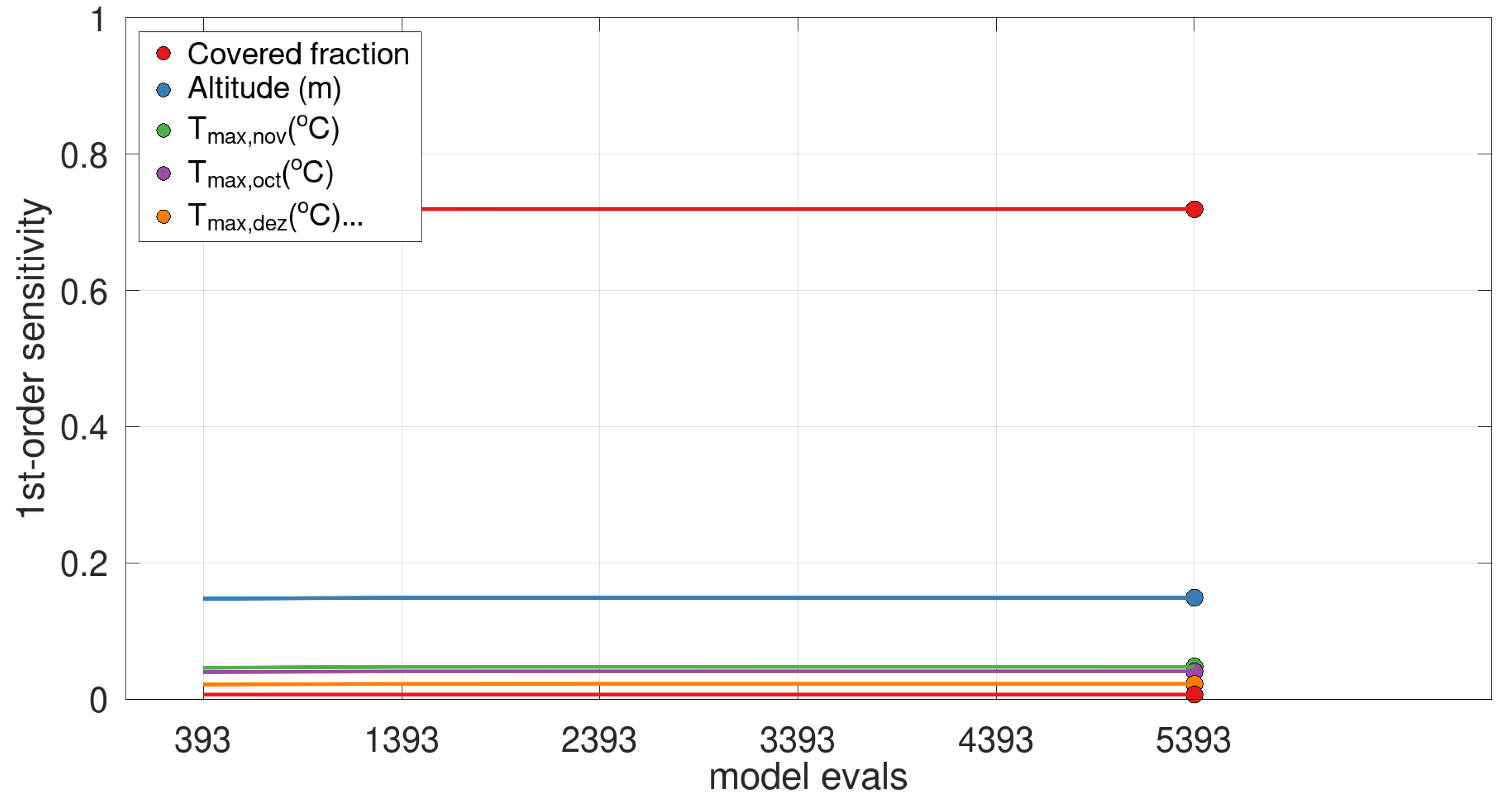
2.3.3. Fourier Amplitude Sensitivity Testing—FAST

Fourier Amplitude Sensitivity Testing (FAST) and the Variance-Based Sensitivity Analysis (VBSA, or Sobol’ method [54]) are variance-based global sensitivity tests [55]. The so-called first-order FAST sensitivity index is calculated by
S i = V i V ( y ) ,
where V i is the first-order conditional variance in Y considering the input X i with a value x i * ( V i = V ( E ( Y | X i = x i * ) ) ) and V ( y ) is the total variance in the model output [56].

2.4. Assumptions of This Study

The following assumptions were made in the present study:
  • The analysis considers only latitude, altitude, the fraction of mulch covering the soil, and the temperatures during three months (October, November, and December) in the water footprint for the wine production;
  • The water footprint only considers the evapotranspiration portion of the viticulture of wine production;
  • Temperatures, relative humidities, and wind speeds are considered to be the same for the different latitudes and altitudes (this assumption may be reasonable considering the small size of the region under consideration; on the other hand, new studies can be conducted considering the uncertainties in temperatures and wind speeds, for instance). Additionally, as already evidenced, the range of variation in the maximum temperatures is higher than the real differences in the regions under study.
As mentioned previously, a large number of studies analyzed the effects of temperatures, relative humidities, and wind speeds in the reference evapotranspiration calculated by the Penman–Monteith model. In our study, we focused on the sensitivity of the model with respect to the parameters that can be effectively chosen by the decision-makers, i.e., the site (latitude and altitude) and the use of a mulch covering.

3. Results

In this section, the results of the computational experiments using the SAFE toolbox applied in the calculation of the water footprint for wine production in the Serra Gaúcha are presented.
The first analysis was conducted with only the sampling strategy and the evaluation of the model, producing a set of scatter plots. Figure 3 presents the scatter plots for the water footprint ( W F , in L/bottle of wine) with respect to the covered fraction, the altitude and the latitude of the site, and to the temperatures over three months. As pointed out by Wang and Solomatine [57], the randomness of the distribution in a scatter plot indicates a low sensitivity, while a prominent pattern points to high sensitivity. In this sense, a clear effect of the covered fraction in the water footprint can be observed. We also noticed that the water footprint was directly affected by the altitude (even considering the nonlinear relationship between the altitude and the reference evapotranspiration). On the other hand, the effects of latitude and of the maximum temperatures for October, November, and December seemed to be less important, according to Figure 3. On the other hand, a direct comparison of the effects is not possible only using the scatter plots. On account of that, the global sensitivity analysis tools must be employed.
First, we considered the calculation of the EE (Morris indexes). Figure 4 illustrates the convergence of the Morris indexes as a function of the number of model evaluations. The convergence with respect to the screening, to the ranking, and to the sensitivity indexes [53] was obtained with a low number of model evaluations.
Figure 5 presents the means and the standard deviations in the EEs for the water footprint calculation. It can be seen that the water footprint is most sensitive to the covered fraction (highest Morris index value, red circle in the figure), followed by the altitude of the site (yellow circle). In addition, it can be concluded that the water footprint is less sensitive (under the assumptions of this study) to the latitude of the location and to the maximum temperatures of the months under consideration.
An important feature of sensitivity analysis is the identification of interactions between parameters. In this sense, Figure 6 presents the interaction effects between the parameters under study, in order to highlight pairwise interactions. As mentioned by Noacco et al. [42] and Puy et al. [58], the existence of clear patterns (a separation of the colors used in the figure colorbars) in the two-dimensional scatter plots indicates an interaction between the corresponding parameters. We observed more expressive interactions between the covered fraction and the other parameters (indicated, for instance, by the yellow points at the left-upper corner of the first line in the figure). The first diagram in Figure 6 indicates that a combination of a low covered fraction and a high altitude (a second-order interaction) implies a maximum response in the water footprint; on the other hand, a high value for the covered fraction in conjunction with a low altitude value (the right-lower corner of this first diagram) minimizes the water footprint. The other parameters did not show an important correlation, i.e., the points/colors are essentially dispersed in the diagrams.
In order to corroborate the results obtained by the EEs, we also employed the FAST sensitivity technique. Figure 7 illustrates the convergence pattern for the FAST indexes for each variable considered in our computations. Clearly, a convergence of the FAST indexes was achieved. In accordance with the results obtained, for instance, in the elementary effects, one can note that the main effects for the covered fraction and for the altitude were more important when compared to the maximum temperatures and to the latitude of the site, since a higher FAST index implies in a higher sensitivity. The accordance of the results obtained by the Morris method and by a Variance-Based Sensitivity Analysis technique (such as FAST) is expected, as pointed out by Campolongo and Cariboni [59]. Furthermore, Paleari et al. [60] identified a concordance of the results (in terms of parameter ranking) obtained by the Morris method and e-FAST, although there was no linearity between the parameters obtained by the two methods.
Table 1 presents the numerical values for the Morris EE (using μ * ) and the FAST indices.

4. Discussion

The results obtained indicate that the water footprint in the viticulture in the Serra Gaúcha (under all the hypotheses considered) is more affected by two parameters—the covered fraction and the altitude—when compared to the other quantities evaluated in the study (latitude and maximum temperatures during the months of October, November, and December). This situation is clearly supported by the results of Figure 3, Figure 5 and Figure 7. These findings are compatible, for instance, with the conclusions of Debnath et al. [18], which obtained an important influence of solar radiation in the reference evapotranspiration (in our computational experiments, this can be noted by the high sensitivity to the altitude of the site). This situation indicates that this kind of approach can be extended to other crops/regions, with the necessary adjustments, in order to predict the particular response (in terms of water footprint), for instance, to severe temperature variations.
It must be emphasized that the effect of the temperatures in the reference evapotranspiration model is absolutely nonlinear, as indicated, for instance, by Equations (A2) and (A8). In the same way, the altitude and latitude of the site also appear in a nonlinear form in the reference evapotranspiration model. Considering this fact, it is clear that some parameters which can be manipulated by the decision-maker are able, for instance, to compensate the effect of temperature variations with respect to the water footprint. To some degree, this situation is similar to that described by Arunrat et al. [20], with respect to some crops in Thailand. As discussed previously, Arunrat et al. [20] argued that the greenhouse effect on the water footprint can be compensated for by an increase in crop productivity. In our numerical experiments, it was shown that this effect (a reduction in the water footprint) can also be produced by an increase in the fraction of vegetation cover, even considering an increase in the temperatures.
With regard to the variables related to a possible decision-making process (covered fraction, altitude and latitude of the site), one can observe that the effect of altitude can be mitigated by the extent of coverage, but only up to a certain threshold (see Figure 6). Secondly, as anticipated, the fraction of mulch covering plays a decisive role across the investigated latitude range. Lower altitudes can decrease the water footprint, even at different latitudes.
It should be clear that the evaluation of the water footprint is extremely important from an environmental point of view, mainly considering climate change. For instance, Saraiva et al. [2] recently discussed, in the form of a review in an initial section of their study, the water footprint of wine production for some Mediterranean countries, highlighting the issue of water scarcity in the region. With respect to the Brazilian case, even considering that we are dealing with a tropical region, the Rio Grande do Sul state is subject to irregular rainfall events [61]. In this sense, a correct understanding of the main variables that are capable of affecting the evapotranspiration and, by consequence, the water footprint, is a fundamental tool both from an environmental point of view and when making decisions to set up a vineyard. Once again, the main finding of this type of analysis is not the direction of the effect (which may be obvious in some cases; for instance, unsurprisingly, an increase in the maximum temperature for a specific month provokes an increase in the water footprint), but the different magnitudes (which may indicate offsetting effects). These magnitudes are indicated, in a pictorial way, by Figure 3 and are proved by the Morris EE and by FAST indexes, according to Table 1.

5. Conclusions

In this work, we conducted a global sensitivity analysis study regarding the water footprint in the viticulture in the Brazilian Serra Gaúcha (only considering the contribution of evapotranspiration to the water footprint). The results indicated that the mulch fraction and the altitude of the site are the two most important parameters in the calculation of the water footprint (under the assumptions of this study). Furthermore, the numerical values obtained using different global sensitivity methods (Morris method and FAST) are consistent and convergent. Our results clearly indicate possible compensation between temperature increase (caused by the greenhouse effect) and the use of vegetation cover. In other words, an increase in the dead mulch covering fraction (a land management technique, and, therefore, a decision) is capable of compensating (in this specific situation) for the impact of the elevation in the temperatures with respect to the water consumption.

Author Contributions

Conceptualization, G.M.P.; methodology, G.M.P., R.G.d.F.C., F.B.S.O., P.R.M. and V.K.N.; software, G.M.P. and P.R.M.; validation, G.M.P., R.G.d.F.C. and F.B.S.O.; formal analysis, G.M.P., R.G.d.F.C. and F.B.S.O.; investigation, G.M.P., R.G.d.F.C., F.B.S.O., P.R.M. and V.K.N.; resources, G.M.P., P.R.M. and V.K.N.; data curation, G.M.P., P.R.M. and V.K.N.; writing—original draft preparation, G.M.P., R.G.d.F.C., F.B.S.O., P.R.M. and V.K.N.; writing—review and editing, G.M.P., R.G.d.F.C., F.B.S.O., P.R.M. and V.K.N.; visualization, G.M.P.; supervision, G.M.P. and F.B.S.O.; project administration, G.M.P. and F.B.S.O. All authors have read and agreed to the published version of the manuscript.

Funding

This study was financed in part by the Coordenação de Aperfeiçoamento de Pessoal de Nível Superior—Brasil (CAPES)—Finance Code 001.

Data Availability Statement

Data are contained within the article.

Conflicts of Interest

The authors declare no conflicts of interest. The funders had no role in the design of the study; in the collection, analyses, or interpretation of data; in the writing of the manuscript; or in the decision to publish the results.

Abbreviations

The following abbreviations are used in this manuscript:
EEelementary effects.
FAOFood and Agriculture Organization.
FASTFourier Amplitude Sensitivity Test.
LHSLatin Hypercube Sampling.
VBSAVariance-Based Sensitivity Analysis.
WFwater footprint.

Appendix A. Evapotranspiration Model

In Equation (1), e s 0 was determined by [12]
e s 0 = e 0 ( T m a x ) + e 0 ( T m i n ) 2 ,
where the saturation pressure is calculated by an Antoine-type equation [12]:
e 0 ( T ) = 0.6108 exp 17.27 T T + 237.3 ,
with the temperature expressed in °C and the vapor pressure calculated in kPa. T m i n and T m a x refer, respectively, to the monthly average daily minimum and maximum temperatures for the months of the year (in °C).
Parameter Δ represents the slope of the saturation pressure curve [12]:
Δ = 4098 0.6108 exp 17.27 T m e a n T m e a n + 237.3 ( T m e a n + 237.3 ) 2 ,
where T m e a n is the mean monthly average temperature.
γ p refers to the psychrometric constant [12]:
γ p = 0.000665 P ,
where P is the local atmospheric pressure (kPa). Here, it was considered that the atmospheric pressure depends on the altitude:
P = 101.3 293 0.0065 z 293 5.26 ,
where z is the site elevation above sea level (m).
The net flux of solar radiation ( R n ) was determined by
R n = R n s R n l ,
where R n s and R n l refer, respectively, to the net short-wave radiation and the net long-wave radiation.
For short-wave radiation, the following expression was employed:
R n s = ( 1 α ) R s ,
where α is the albedo coefficient ( α = 0.23 , as pointed out by [12]) and R s is the incident solar radiation.
The long-wave radiation was calculated by [12]
R n l = σ f c d 0.34 0.14 e a T K , m a x 4 + T K , m i n 4 2 ,
where σ is the Stefan–Boltzmann constant, and f c d is the cloudiness function. T K , m a x and T K , m i n , respectively, refer to the monthly average daily maximum and minimum absolute temperatures (for a specific month of the year). The cloudiness function f c d was evaluated by
f c d = 1.35 R s R s 0 0.35 ,
where R s 0 is the solar radiation in the absence of clouds (clear sky). Values of R s 0 can be obtained by using information regarding the extraterrestrial radiation ( R a ). For instance, R s 0 = ( 0.75 + 2 × 10 5 z ) R a , where z is the site elevation with respect to the sea level.
The extraterrestrial radiation R a (short-wave radiation in the absence of an atmosphere, or solar radiation at the top of the atmosphere) was calculated by
R a = 24 × 60 π G s c d r ω s sin ( γ ) sin ( δ ) + cos ( γ ) cos ( δ ) sin ( ω s ) ,
where γ is the latitude (rad) and δ represents the declination (rad). In Equation (A10), G s c is the solar constant 0.0820 M J m 2 m i n , d r is the inverse relative distance earth–sun, calculated by
d r = 1 + 0.033 cos 2 π 365 J ,
where J = i n t ( 30.4 M 15 ) (Julian day). Moreover, J is the day halfway through the month, i n t is the integer function, and M is the month under consideration. The solar declination δ was calculated by
δ = 0.409 sin 2 π 365 J 1.39 ,
The incident solar radiation was evaluated by
R s = a s + b s n N R a ,
where a s = 0.25 and b s = 0.50 [62]. Furthermore, n is the number of hours of sunlight per day and N is the maximum number of sunlight hours per day N = 24 π ω s . The parameter ω s (solar angle at the end of the day) was calculated by ω s = arccos tan ( γ ) tan ( δ ) .
The actual vapor pressure ( e a ) can be obtained using relative humidity data ( U R ) [12], according to
e a = U R m e a n 100 e 0 ( T m a x ) + e 0 ( T m i n ) 2 ,
Finally, in Equation (1), G is the heat flux in the soil, calculated by [12]
G = 0.07 T m o n t h , i + 1 T m o n t h , i 1 ,
where T m o n t h , i refers to the mean air temperature of the month i. It can be noted that the calculation of the soil heat flux G demands information regarding the mean air temperature of every month of the year. On the other hand, as mentioned by Martins [63], the value of G can be approximated using the simple arithmetic mean between the maximum and minimum temperatures for a month as a good approach. In fact, in many cases, is reasonable to accept that G 0 [12].

References

  1. Finco, A.; Bentivoglio, D.; Chiaraluce, G.; Alberi, M.; Chiarelli, E.; Maino, A.; Mantovani, F.; Montuschi, M.; Raptis, K.G.C.; Semenza, F.; et al. Combining Precision Viticulture Technologies and Economic Indices to Sustainable Water Use Management. Water 2022, 14, 1493. [Google Scholar] [CrossRef]
  2. Saraiva, A.; Presumido, P.; Silvestre, J.; Feliciano, M.; Rodrigues, G.; Silva, P.O.e.; Damásio, M.; Ribeiro, A.; Ramôa, S.; Ferreira, L.; et al. Water Footprint Sustainability as a Tool to Address Climate Change in the Wine Sector: A Methodological Approach Applied to a Portuguese Case Study. Atmosphere 2020, 11, 934. [Google Scholar] [CrossRef]
  3. Wurz, D.A.; Brighenti, A.F. Analysis of Brazilian wine competitiveness. BIO Web Conf. 2019, 12, 03015. [Google Scholar] [CrossRef]
  4. Alderete, M.V. The Wine Clusters of Mendoza and Serra Gaúcha: A Local Development Perspective. Front. Norte 2014, 26, 179–204. (In Spanish) [Google Scholar]
  5. Zen, A.C.; Fensterseifer, J.E.; Prévot, F. The influence of resources on the internationalisation process of clustered wine companies. Int. J. Bus. Glob. 2012, 8, 30–48. [Google Scholar] [CrossRef]
  6. Fensterseifer, J.E. The emerging Brazilian wine industry: Challenges and prospects for the Serra Gaúcha wine cluster. Int. J. Wine Bus. Res. 2007, 19, 187–206. [Google Scholar] [CrossRef]
  7. Hoekstra, A.; Hung, P. Virtual Water Trade: A Quantification of Virtual Water Flows between Nations in Relation to International Crop Trade; Value of Water. Research Report Series No. 11; IHL Delft: Delft, The Netherlands, 2002. [Google Scholar]
  8. Herath, I.; Green, S.; Singh, R.; Horne, D.; van der Zijpp, S.; Clothier, B. Water footprinting of agricultural products: A hydrological assessment for the water footprint of New Zealand’s wines. J. Clean. Prod. 2013, 41, 232–243. [Google Scholar] [CrossRef]
  9. Bonamente, E.; Scrucca, F.; Asdrubali, F.; Cotana, F.; Presciute, A. The Water Footprint of the Wine Industry: Implementation of an Assessment Methodology and Application to a Case Study. Sustentability 2015, 7, 12190–12208. [Google Scholar] [CrossRef]
  10. Jairman, C. Water Footprint as an Indicator of Sustainable Table and Wine Grape Production; Technical Report; Water Research Comission: Gezina, South Africa, 2020. [Google Scholar]
  11. Saraiva, A.; Rodrigues, G.; Silvestre, J.; Feliciano, M.; Silva, P.; Oliveira, M. A pegada hídrica na fileira vitivinícola portuguesa. Agrotec 2019, 35, 68–70. (In Portuguese) [Google Scholar]
  12. Allen, R.; Walter, I.; Elliot, R.; Howell, T.; Itenfisu, D.; Jensen, M. The ASCE Standardized Reference Evapotranspiration Equation; ASCE: Reston, VA, USA, 2005. [Google Scholar]
  13. Adib, A.; Kalantarzadeh, S.S.O.; Shoushtari, M.M.; Lotfirad, M.; Liaghat, A.; Oulapour, M. Sensitive analysis of meteorological data and selecting appropriate machine learning model for estimation of reference evapotranspiration. Appl. Water Sci. 2023, 13, 83. [Google Scholar] [CrossRef]
  14. Ndiaye, P.; Bodian, A.; Diop, L.; Djaman, K. Sensitivity Analysis of the Penman-Monteith Reference Evapotranspiration to Climatic Variables: Case of Burkina Faso. J. Water Resour. Prot. 2017, 9, 1364–1376. [Google Scholar] [CrossRef]
  15. Ndiaye, P.M.; Bodian, A.; Diop, L.; Dezetter, A.; Guilpart, E.; Deme, A.; Ogilvie, A. Future trend and sensitivity analysis of evapotranspiration in the Senegal River Basin. J. Hydrol. Reg. Stud. 2021, 35, 100820. [Google Scholar] [CrossRef]
  16. Beven, K. A Sensitivity Analysis of the Penman-Monteith Actual Evapotranspiration Estimates. J. Hydrol. 1979, 44, 169–190. [Google Scholar] [CrossRef]
  17. Irmak, S.; Payero, J.O.; Martin, D.L.; Irmak, A.; Howell, T.A. Sensitivity Analyses and Sensitivity Coefficients of Standardized Daily ASCE-Penman-Monteith Equation. J. Irrig. Drain. Eng. 2006, 132, 564–578. [Google Scholar] [CrossRef]
  18. Debnath, S.; Adamala, S.; Raghuwanshi, N. Sensitivity Analysis of FAO-56 Penman-Monteith Method for Different Agro-ecological Regions of India. Environ. Process. 2015, 2, 689–704. [Google Scholar] [CrossRef]
  19. Biazar, S.M.; Dinpashoh, Y.; Singh, V.P. Sensitivity analysis of the reference crop evapotranspiration in a humid region. Environ. Sci. Pollut. Res. 2019, 26, 32517–32544. [Google Scholar] [CrossRef] [PubMed]
  20. Arunrat, N.; Sereenonchai, S.; Chaowiwat, W.; Wang, C. Climate change impact on major crop yield and water footprint under CMIP6 climate projections in repeated drought and flood areas in Thailand. Sci. Total Environ. 2022, 807, 150741. [Google Scholar] [CrossRef] [PubMed]
  21. Rossi, L.; Regni, L.; Rinaldi, S.; Sdringola, P.; Calisti, R.; Brunori, A.; Dini, F.; Proietti, P. Long-Term Water Footprint Assessment in a Rainfed Olive Tree Grove in the Umbria Region, Italy. Agriculture 2020, 10, 8. [Google Scholar] [CrossRef]
  22. Arunrat, N.; Sereenonchai, S.; Chaowiwat, W.; Wang, C.; Hatano, R. Carbon, Nitrogen and Water Footprints of Organic Rice and Conventional Rice Production over 4 Years of Cultivation: A Case Study in the Lower North of Thailand. Agronomy 2022, 12, 380. [Google Scholar] [CrossRef]
  23. Yong, S.L.S.; Ng, J.L.; Huang, Y.F.; Ang, C.K.; Mirzaei, M.; Ahmed, A.N. Local and global sensitivity analysis and its contributing factors in reference crop evapotranspiration. Water Supply 2023, 23, 1672–1683. [Google Scholar] [CrossRef]
  24. Sabino, M.; de Souza, A.P. Global Sensitivity of Penman–Monteith Reference Evapotranspiration to Climatic Variables in Mato Grosso, Brazil. Earth 2023, 4, 714–727. [Google Scholar] [CrossRef]
  25. Zhuo, L.; Mekonnen, M.M.; Hoekstra, A.Y. Sensitivity and Uncertainty in Crop Water Footprint Accounting: A Case Study for the Yellow River Basin; Value of Water Research Report Series no. 62; UNESCO–IHE; Enschede: Delft, The Nethelands, 2013. [Google Scholar]
  26. Li, Z.; Feng, B.; Wang, W.; Yang, X.; Wu, P.; Zhuo, L. Spatial and temporal sensitivity of water footprint assessment in crop production to modelling inputs and parameters. Agric. Water Manag. 2022, 271, 107805. [Google Scholar] [CrossRef]
  27. Conceição, M.A.F.; Mandelli, F. Climate trends in the Serra Gaúcha region. In Proceedings of the XV Brazilian Congress on Agrometereology, Aracaju, Brazil, 2–5 July 2007. (In Portuguese). [Google Scholar]
  28. Cardoso, I.P.; Siqueira, T.M.; Timm, L.C.; Rodrigues, A.A.; Nunes, A.B. Analysis of average annual temperatures and rainfall in southern region of the state of Rio Grande do Sul, Brazil. Braz. J. Environ. Sci. (RBCIAMB) 2022, 57, 58–71. [Google Scholar] [CrossRef]
  29. Lu, J.; Sun, G.; McNulty, S.G.; Amatya, D.M. A comparison of six potential evapotranspiration methods for regional use in the Southeastern United States. JAWRA J. Am. Water Resour. Assoc. 2005, 41, 621–633. [Google Scholar] [CrossRef]
  30. Mobilia, M.; Longobardi, A. Prediction of Potential and Actual Evapotranspiration Fluxes Using Six Meteorological Data-Based Approaches for a Range of Climate and Land Cover Types. ISPRS Int. J. Geo-Inf. 2021, 10, 192. [Google Scholar] [CrossRef]
  31. Yang, Y.; Chen, R.; Han, C.; Liu, Z. Evaluation of 18 models for calculating potential evapotranspiration in different climatic zones of China. Agric. Water Manag. 2021, 244, 106545. [Google Scholar] [CrossRef]
  32. Sentelhas, P.C.; Gillespie, T.J.; Santos, E.A. Evaluation of FAO Penman–Monteith and alternative methods for estimating reference evapotranspiration with missing data in Southern Ontario, Canada. Agric. Water Manag. 2010, 97, 635–644. [Google Scholar] [CrossRef]
  33. Eaton, J.W.; Bateman, D.; Hauberg, S.; Wehbring, R. GNU Octave Version 8.3.0 Manual: A High-Level Interactive Language for Numerical Computations. 2023. [Google Scholar]
  34. Pianosi, F.; Sarrazin, F.; Wagener, T. A Matlab toolbox for Global Sensitivity Analysis. Environ. Model. Softw. 2015, 70, 80–85. [Google Scholar] [CrossRef]
  35. Borges, L.F.A.; Ferreira, F.F.; Gonçalves, F.; Espósito Junior, A.; Oliveira, A.F.d.S.; Telles, W.R. IPSAL: Implementation of the module to generate the Sobol sequence and indices. VETOR 2023, 33, 60–69. [Google Scholar] [CrossRef]
  36. Li, S.; Li, Y.; Lin, H.; Feng, H.; Dyck, M. Effects of different mulching technologies on evapotranspiration and summer maize growth. Agric. Water Manag. 2018, 201, 309–318. [Google Scholar] [CrossRef]
  37. Fonseca, M.A. Models to Estimate the Crop Coefficients (Kc) for Irrigated Grapevines; Embrapa: Bento Gonçalves, Brazil, 2016. (In Portuguese) [Google Scholar]
  38. Rosa, J.D.; Mafra, Á.L.; Nohatto, M.A.; Ferreira, E.Z.; de Oliveira, O.L.P.; Miquelluti, D.J.; Cassol, P.C.; Medeiros, J.C. Soil chemical properties and grapevine yield affected by cover crop management in Serra Gaúcha, Southern Brazil. Rev. Bras. Ciência Solo 2009, 33, 179–187. (In Portuguese) [Google Scholar] [CrossRef]
  39. López-Urrea, R.; Sánchez, J.; Montoro, A.; Mañas, F.; Intrigliolo, D. Effect of using pruning waste as an organic mulching on a drip-irrigated vineyard evapotranspiration under a semi-arid climate. Agric. For. Meteorol. 2020, 291, 108064. [Google Scholar] [CrossRef]
  40. Mirás-Avalos, J.M.; Araujo, E.S. Optimization of Vineyard Water Management: Challenges, Strategies, and Perspectives. Water 2021, 13, 746. [Google Scholar] [CrossRef]
  41. Lazzarotto, J.J.; Protas, J.F.S. Capital Costs and Demands for the Production of Vineyards for Processing in Bento Gonçalves on a Spaleswood; Observatórios Agropensa: Bento Gonçalves, Brazil, 2020; pp. 1–10. (In Portuguese) [Google Scholar]
  42. Noacco, V.; Sarrazin, F.; Pianosi, F.; Wagener, T. Matlab/R workflows to assess critical choices in Global Sensitivity Analysis using the SAFE toolbox. MethodsX 2019, 6, 2258–2280. [Google Scholar] [CrossRef]
  43. Viana, F.A.C. A Tutorial on Latin Hypercube Design of Experiments. Qual. Reliab. Eng. Int. 2016, 32, 1975–1985. [Google Scholar] [CrossRef]
  44. Jung, C.G.; Lee, D.R.; Moon, J.W. Comparison of the Penman-Monteith method and regional calibration of the Hargreaves equation for actual evapotranspiration using SWAT-simulated results in the Seolma-cheon basin, South Korea. Hydrol. Sci. J. 2016, 61, 793–800. [Google Scholar] [CrossRef]
  45. Demirel, M.C.; Koch, J.; Mendiguren, G.; Stisen, S. Spatial Pattern Oriented Multicriteria Sensitivity Analysis of a Distributed Hydrologic Model. Water 2018, 10, 1188. [Google Scholar] [CrossRef]
  46. Beyene, T.D.; Zimale, F.A.; Gebrekristos, S.T.; Nedaw, D. Assessment of the impact of rainfall uncertainties on the groundwater recharge estimations of the Tikur-Wuha watershed, rift valley lakes basin, Ethiopia. Heliyon 2024, 10, e24311. [Google Scholar] [CrossRef] [PubMed]
  47. Pang, M.; Xu, R.; Hu, Z.; Wang, J.; Wang, Y. Uncertainty and Sensitivity Analysis of Input Conditions in a Large Shallow Lake Based on the Latin Hypercube Sampling and Morris Methods. Water 2021, 13, 1861. [Google Scholar] [CrossRef]
  48. Sheikholeslami, R.; Razavi, S. Progressive Latin Hypercube Sampling: An efficient approach for robust sampling-based analysis of environmental models. Environ. Model. Softw. 2017, 93, 109–126. [Google Scholar] [CrossRef]
  49. Morris, M.D. Factorial Sampling Plans for Preliminary Computational Experiments. Technometrics 1991, 33, 161–174. [Google Scholar] [CrossRef]
  50. Campolongo, F.; Saltelli, A.; Cariboni, J. From screening to quantitative sensitivity analysis. A unified approach. Comput. Phys. Commun. 2011, 182, 978–988. [Google Scholar] [CrossRef]
  51. Tian, W.; Song, J.; Li, Z.; de Wilde, P. Bootstrap techniques for sensitivity analysis and model selection in building thermal performance analysis. Appl. Energy 2014, 135, 320–328. [Google Scholar] [CrossRef]
  52. Campolongo, F.; Cariboni, J.; Saltelli, A. An effective screening design for sensitivity analysis of large models. Environ. Model. Softw. 2007, 22, 1509–1518. [Google Scholar] [CrossRef]
  53. Sarrazin, F.; Pianosi, F.; Wagener, T. Global Sensitivity Analysis of environmental models: Convergence and validation. Environ. Model. Softw. 2016, 79, 135–152. [Google Scholar] [CrossRef]
  54. Sobol, I. Global sensitivity indices for nonlinear mathematical models and their Monte Carlo estimates. Math. Comput. Simul. 2001, 55, 271–280. [Google Scholar] [CrossRef]
  55. Saltelli, A.; Bolado, R. An alternative way to compute Fourier amplitude sensitivity test (FAST). Comput. Stat. Data Anal. 1998, 26, 445–460. [Google Scholar] [CrossRef]
  56. Yan, M.; Tian, X.; Li, Z.; Chen, E.; Wang, X.; Han, Z.; Sun, H. Simulation of Forest Carbon Fluxes Using Model Incorporation and Data Assimilation. Remote Sens. 2016, 8, 567. [Google Scholar] [CrossRef]
  57. Wang, A.; Solomatine, D.P. Practical Experience of Sensitivity Analysis: Comparing Six Methods, on Three Hydrological Models, with Three Performance Criteria. Water 2019, 11, 1062. [Google Scholar] [CrossRef]
  58. Puy, A.; Lo Piano, S.; Saltelli, A.; Levin, S.A. sensobol: An R Package to Compute Variance-Based Sensitivity Indices. J. Stat. Softw. 2022, 102, 1–37. [Google Scholar] [CrossRef]
  59. Campolongo, F.; Cariboni, J. On the Relationship Between the Sensitivity Measures Proposed by Morris and the Variance Based Measures. In Proceedings of the Probabilistic Safety Assessment and Management; Spitzer, C., Schmocker, U., Dang, V.N., Eds.; Springer: London, UK, 2004; pp. 2030–2035. [Google Scholar] [CrossRef]
  60. Paleari, L.; Movedi, E.; Zoli, M.; Burato, A.; Cecconi, I.; Errahouly, J.; Pecollo, E.; Sorvillo, C.; Confalonieri, R. Sensitivity analysis using Morris: Just screening or an effective ranking method? Ecol. Model. 2021, 455, 109648. [Google Scholar] [CrossRef]
  61. Valente, P.T.; Viana, D.R.; Aquino, F.E.; Simões, J.C. Classification of precipitation anomalies in the Rio Grande do Sul in ENSO events in the 20th century. Soc. Nat. 2023, 35, e66073. [Google Scholar] [CrossRef]
  62. Allen, R.G.; Pereira, L.S.; Raes, D.; Smith, M. FAO Irrigation and Drainage Paper No. 56–Crop Evapotranspiration (Guidelines for Computing Crop Water Requirements); Technical Report; FAO: Rome, Italy, 1998. [Google Scholar]
  63. Martins, P.R. Water Footprint Modelling in Viticulture for the Wine Production in the Serra Gaúcha. Master’s Thesis, Graduate Program in Agroindustrial Systems and Processes, Federal University of Rio Grande, Santo Antônio da Patrulha, Brazil, 2023. Available online: https://argo.furg.br/?BDTD13706 (accessed on 19 March 2024). (In Portuguese).
Figure 1. Altimetric map of Rio Grande do Sul, Brazil, and localization map of Serra Gaúcha.
Earth 05 00007 g001
Figure 2. Maximum temperatures for the months of October, November, and December in the Serra Gaúcha (2013–2023).
Earth 05 00007 g002
Figure 3. Scatterplots (inputs–output) for the water footprint (L/bottle of wine) considering the uncertainties in the soil-covered fraction (dimensionless), altitude (m), and latitude. N = 3000 .
Earth 05 00007 g003
Figure 4. Means of Morris elementary effects (EEs) convergence patterns.
Earth 05 00007 g004
Figure 5. Elementary effects (EEs) for the water footprint (L/bottle of wine) with r = 500 and N b o o t = 100 .
Earth 05 00007 g005
Figure 6. Scatter plots (interaction effects) for the water footprint (L/bottle of wine).
Earth 05 00007 g006
Figure 7. Convergence pattern of main effects or first-order effects using FAST.
Earth 05 00007 g007
Table 1. Morris EE effects and FAST indices for the water footprint.
Morris EE ( μ * )FAST Index
Covered fraction34.20177.1938 × 10 1
Altitude15.28321.4891 × 10 1
Latitude2.90886.5333 × 10 3
T m a x , o c t 7.66364.0507 × 10 2
T m a x , n o v 8.31524.7451 × 10 2
T m a x , d e c 5.99912.2368 × 10 2
Disclaimer/Publisher’s Note: The statements, opinions and data contained in all publications are solely those of the individual author(s) and contributor(s) and not of MDPI and/or the editor(s). MDPI and/or the editor(s) disclaim responsibility for any injury to people or property resulting from any ideas, methods, instructions or products referred to in the content.

