SPH Simulation of Molten Metal Flow Modeling Lava Flow Phenomena with Solidification

Abstract

Characteristic dynamics in lava flows, such as the formation processes of lava levees, toe-like tips, and overlapped structures, were reproduced successfully through numerical simulation using the smoothed particle hydrodynamics (SPH) method. Since these specific phenomena have a great influence on the flow direction of lava flows, it is indispensable to elucidate them for accurate predictions of areas where lava strikes. At the first step of this study, lava was expressed using a molten metal with known physical properties. The computational results showed that levees and toe-like tips formed at the fringe of the molten metal flowing down on a slope, which appeared for actual lava flows as well. The dynamics of an overlapped structure formation were also simulated successfully; therein, molten metal flowed down, solidified, and changed the surface shape of the slope, and the second molten metal flowed over the changed surface shape. It was concluded that the computational model developed in this study using the SPH method is applicable for simulating and clarifying lava flow phenomena.

1. Introduction

Volcanic eruptions accompanied by lava flows often occur in various volcanos and have caused extensive damage to the areas where the lava flowed. Volcanic eruptions in Iceland in 2023–2024 caused damage to a nearby town because of a lava flow. In order to mitigate damage by lava flows, it is necessary to accurately predict areas where the lava flows by taking measures such as city planning and creating hazard maps based on these predictions. Elucidating the characteristics of lava and specific lava flow phenomena, and considering them in predictions, are essential steps for more accurate predictions. Therefore, a lot of studies have been conducted [1,2,3,4,5,6,7,8,9,10,11,12,13].

These previous studies include field studies, experimental studies using wax, which is similar to lava in terms of crust formation due to surface cooling and solidification [1,2], and numerical simulations. Field studies are hazardous, and opportunities for them are limited because volcanic eruptions with lava flows are infrequent phenomena. Furthermore, it is difficult to clarify the behaviors of a convective flow and heat transfer with solidification in and on the surface of lava through such field and experimental studies because those of actual lava flows are hard to observe and measure directly and are affected by various factors interacting with each other. Therefore, numerical simulation is effective in reproducing and elucidating lava flow phenomena.

Some characteristic phenomena are observed in a lava flow. The lava changes from a Newtonian fluid to a more complex fluid due to suspended crystals and gas bubbles [3]. Moreover, a toe-like shape and a lava levee are formed. Hon et al. photographed the tip shape of solidified lava at Mt. Kilauea (See Figure 2c in Ref. [4]). In this photograph, a toe-like structure had formed at the tip of the lava. The lava was overlapped because new lava flowed on the solidified lava. It is known that solidified lava causes the accretion of the topography and affects the flow direction of following lava flows.

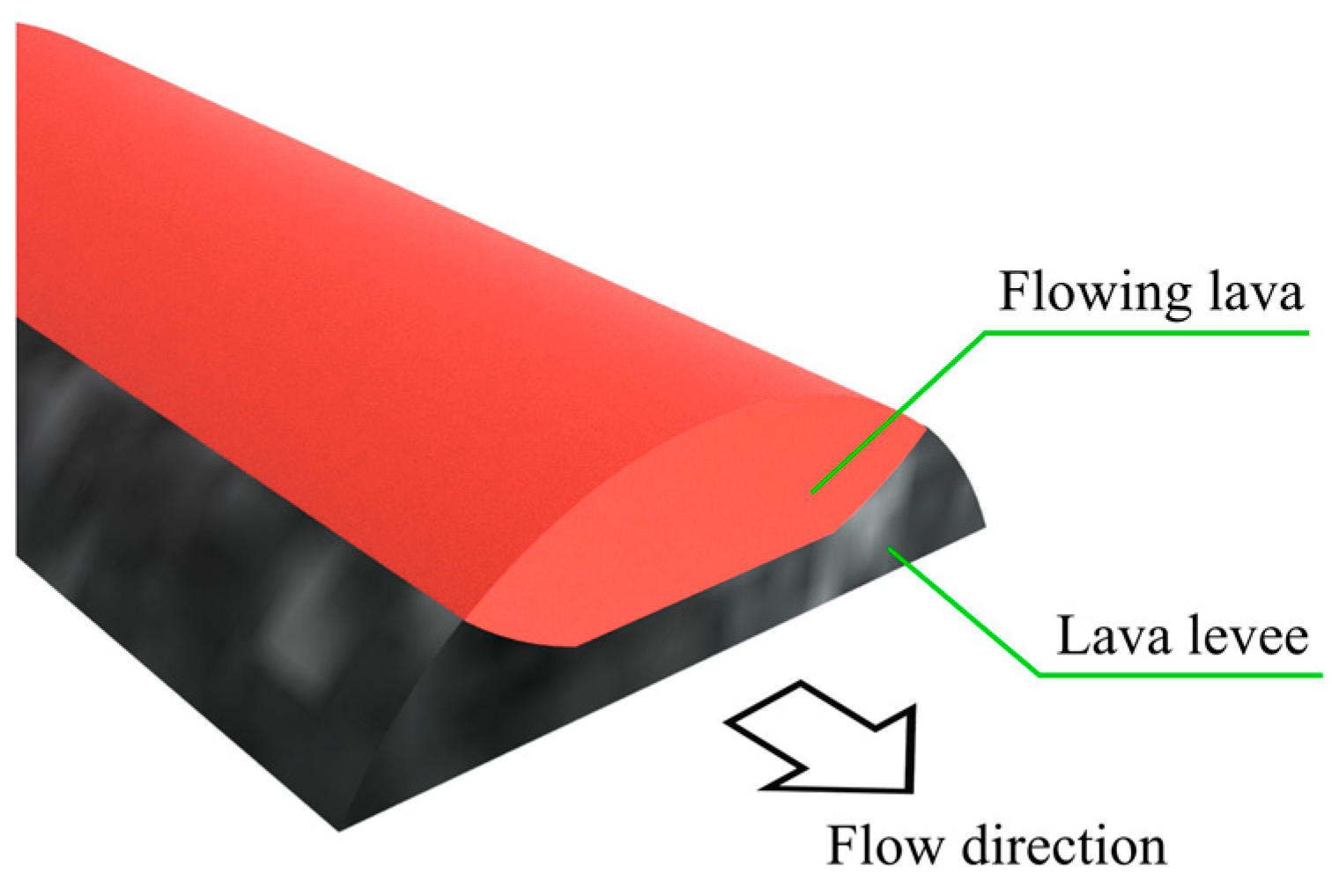
The lava levee is a levee-like structure. The outside and bottom of a lava flow are easily cooled and solidified. On the other hand, the inside lava flows without solidifying for a relatively long distance due to its low cooling rate. Because of differences in the cooling rate, a levee-like topography is formed. Figure 1 shows a schematic of a cross-section of a lava levee. The formation process of lava levees has a great influence on the flow direction of lava flows. Therefore, clarification of the formation process will improve the accuracy of predicting areas where lava flows.

The complex viscosity, the solidification of lava, and the deformation of the solid–liquid interfaces make numerical simulations difficult. Some previous studies [14,15,16,17] proposed methods to simulate the behavior of non-Newtonian fluids. Some previous studies [5,6,7] took a simplified approach to the solidification of lava and the deformation of the solid–liquid interfaces. For example, Tsepelev et al. [6] represented crust formation and fracture at the lava surface by introducing rafts directly onto the fluid without considering heat transports. Mesh-based computational methods such as finite volume and finite element methods have the disadvantage of requiring remeshing because of the deformation of the solid–liquid interfaces and lava flow itself [6,8]. Therefore, a smoothed particle hydrodynamics (SPH) method, which is one of the mesh-free methods, is useful for reproducing these phenomena. Previous studies [18,19,20,21,22] have attempted to apply an SPH method to non-Newtonian fluids. Lava flow simulations that take into account non-Newtonian behavior and viscous changes have also been conducted [9,10,11,12,13]. On the other hand, only a few reports have considered heat transport and solid–liquid phase changes in lava flow phenomena.

Lan et al. [23] proposed an SPH method that considers solid–liquid phase changes to simulate the spreading and solidification of nuclear reactor core melting. In this study, the formation of crust at the surface of the flow was reproduced. However, the levee-like shape and accretion were not observed. Zago et al. [10,11,12] conducted simulations considering heat transport and solid–liquid phase changes for lava flow phenomena. However, their simulation did not reproduce the lava levees or accretion. Hérault et al. [13] simulated a lava flow on the topography of Mt. Etna considering heat transport and solid–liquid phase changes. They succeeded in reproducing the lava levees formed on the sides of the lava flow. However, the discussion on its shape and elucidation of its formation process were not enough. They mentioned the representation of accretion. However, its actual reproduction in the simulation was not mentioned, and its influence on the following flow was not discussed.

Therefore, the eventual goal of this study was to simulate and clarify specific lava flow phenomena such as lava levees and lava overlapping in order to improve the prediction accuracy of inflow areas. As the first step, this study aimed to verify the feasibility of simulating lava flows with solidification. For simplicity, lava flows on a tilted surface were modeled with molten metal, with physical properties that are easily obtained, and treated as Newtonian fluid with constant viscosity.

2. Computational Method

2.1. Governing Equations

In this study, the computational object is the flow of molten metal and its solidification. The governing equations for molten metal are as follows. The continuity equation for a flow with constant density is expressed as

$$\nabla ·\stackrel{⃑}{u}=0,$$

(1)

where $\stackrel{⃑}{u}$ is the velocity. The Lagrange form of the Navier–Stokes equation for describing the motion of a flow with constant density and viscosity is given by

$$\frac{D\stackrel{⃑}{u}}{Dt}=-\frac{1}{\rho }\nabla p+\frac{\mu }{\rho }{\nabla }^2\stackrel{⃑}{u}+\frac{\stackrel{⃑}{F}}{\rho },$$

(2)

where $t$ is the time, $\rho$ is the density, $p$ is the pressure, $\mu$ is the constant viscosity, and $\stackrel{⃑}{F}$ is the external force, which includes buoyancy force and surface tension force with temperature dependence. The lava changes from Newtonian fluid to a more complex fluid due to suspended crystals and gas bubbles [3]. However, a previous study [24] indicated that melted silicate can be treated as a Newtonian fluid under a wide range of phenomena. Moreover, another study [25] showed that melted silicate can be treated as Newtonian fluids when the crystal fraction in the melted silicate is low. This study focused on lava levees and accretion due to heat transport and solid–liquid phase changes in lava, which were not sufficiently discussed in previous studies. Therefore, the lava was simplified as a Newtonian fluid with constant viscosity for a more low-cost model.

The energy transport equation for the temperature change in a fluid is written as

$$\frac{DT}{Dt}=\frac{1}{\rho C}\nabla ·\left(\kappa \nabla T\right)+\frac{Q}{\rho C},$$

(3)

where $T$ is the temperature, $C$ is the specific heat, $\kappa$ is the temperature-dependent thermal conductivity, and $Q$ is the heat generation rate, which involves the heat flux to the ambient gas, radiation on the surface, and heat input for generating molten metal.

2.2. Discretization of Governing Equations in SPH Method

In the SPH method, the physical quantity $\varphi$ defined on particle $a$ located at ${\stackrel{⃑}{r}}_a(x,y,z)$ is described using the following equation, considering the effect of the neighbor particles $b$ [26]:

$${\varphi }_{(\stackrel{⃑}{r}={\stackrel{⃑}{r}}_a)}=\sum _b{m}_b\frac{{\varphi }_b}{{\rho }_b}{W}_{ab},$$

(4)

where $m$ is the mass, and $W$ is the kernel function that expresses the spread of the physical quantity of a particle. This function is determined using the particle diameter $h$ and the distance between particles $a$ and $b$, $\left|{\stackrel{⃑}{r}}_{ab}\right|=\left|{\stackrel{⃑}{r}}_a-{\stackrel{⃑}{r}}_b\right|$. In this study, the M4 spline function for a three-dimensional space was used as the kernel function [26].

In the SPH method used in this study, there is no need to explicitly treat the continuity equation because the mass of particles is constant and the number of particles in the computational domain is conserved. Therefore, the Navier–Stokes equation and the energy transport equation are solved.

2.2.1. Discretization of Navier–Stokes Equation

In discretizing Equation (2) using the SPH method, the following equation is obtained:

$$\frac{D{\stackrel{⃑}{u}}_a}{Dt}=-\sum _b{m}_b\left(\frac{p_a}{{\rho }_a^2}+\frac{p_b}{{\rho }_b^2}\right)\nabla W_{ab}+\frac{2\delta }{{\lambda }_a{n}_a{\rho }_a}\mu \sum _b\left({\stackrel{⃑}{u}}_b-{\stackrel{⃑}{u}}_a\right)W_{ab}+\frac{{\stackrel{⃑}{F}}_a}{{\rho }_a},$$

(5)

where $\delta$ is the number of dimensions of the computational domain, $\lambda$ is the parameter in the moving particle semi-implicit (MPS) method, and $n$ is the number density. The first term on the right-hand side in Equation (5) is the pressure gradient term. It is discretized to satisfy the action–reaction law. In this simulation, this term is replaced by the algorithm of incompressibility described in Section 2.2.2. The second term on the right-hand side is the viscosity term. It is discretized using the Laplacian model of the MPS method [27]. The third term on the right-hand side is the external force term, which includes buoyancy force and surface tension force with temperature dependence. The surface tension force acting on the interface can be divided into a normal component, which appears as the Laplace pressure, and a tangential component, which appears as the Marangoni effect due to the surface tension gradient. Therefore, external force ${\stackrel{⃑}{F}}_a$ is expressed as

$${\stackrel{⃑}{F}}_a={\stackrel{⃑}{F}}_a^{\mathrm{L}}+{\stackrel{⃑}{F}}_a^{\mathrm{M}}+{\stackrel{⃑}{F}}_a^{\mathrm{B}},$$

(6)

where ${\stackrel{⃑}{F}}_a^{\mathrm{L}}$ is the normal surface tension force, ${\stackrel{⃑}{F}}_a^{\mathrm{M}}$ is the tangential surface tension force, and ${\stackrel{⃑}{F}}_a^{\mathrm{B}}$ is the buoyancy force.

The normal surface tension force is modeled as an inter-particle attraction and formulated as follows [28]:

$${\stackrel{⃑}{F}}_a^{\mathrm{L}}=\frac{1.2\gamma h}{V_a}\sum _{b\ne a}{\stackrel{⃑}{f}}_{ab}^{\mathrm{a}\mathrm{t}\mathrm{t}\mathrm{r}\mathrm{a}\mathrm{c}\mathrm{t}},$$

(7)

where $\gamma$ is the surface tension coefficient, and $V$ is the volume of the computational particle. ${\stackrel{⃑}{f}}_{ab}^{\mathrm{a}\mathrm{t}\mathrm{t}\mathrm{r}\mathrm{a}\mathrm{c}\mathrm{t}}$ is the following weight function obtained using the distance $\left|{\stackrel{⃑}{r}}_{ab}\right|$:

$${\stackrel{⃑}{f}}_{ab}^{\mathrm{a}\mathrm{t}\mathrm{t}\mathrm{r}\mathrm{a}\mathrm{c}\mathrm{t}}\left(\left|{\stackrel{⃑}{r}}_{ab}\right|,h\right)=\left\{\begin{array}{cc}\frac{\left|{\stackrel{⃑}{r}}_{ab}\right|}{h}& \left(0\le \left|{\stackrel{⃑}{r}}_{ab}\right|<h\right)\\ 2-\frac{\left|{\stackrel{⃑}{r}}_{ab}\right|}{h}& \left(h\le \left|{\stackrel{⃑}{r}}_{ab}\right|<2h\right)\\ 0& \left(2h\le \left|{\stackrel{⃑}{r}}_{ab}\right|\right)\end{array}\right..$$

(8)

In this model, Ito et al. [28] confirmed that when the surface tension coefficient is set to a function of temperature, the inter-particle stress becomes unbalanced, which finally causes a reduction in computational accuracy. Therefore, the surface tension coefficient was set to be constant without considering the temperature dependence to avoid reducing the computational accuracy.

On the other hand, in modeling a tangential surface tension, the temperature dependence of the surface tension is taken into account because the force is caused by the temperature gradient in the surface tension. It is expressed as

$${\stackrel{⃑}{F}}_a^{\mathrm{M}}=\frac{\partial \gamma }{\partial T}\frac{S_a\left[\left({\stackrel{⃑}{\eta }}_a\times {\nabla T}_a\right)\times {\stackrel{⃑}{\eta }}_a\right]}{V_a},$$

(9)

where $S$ is the cross-sectional area through the center of the computational particle, and $\stackrel{⃑}{\eta }$ is the unit vector normal to the interface.

The buoyancy force is formulated using the Boussinesq approximation as follows:

$${\stackrel{⃑}{F}}_a^{\mathrm{B}}=\left(T_a-T_0\right)\beta {\rho }_a\stackrel{⃑}{g},$$

(10)

where $T_0$ is the reference temperature, $\beta$ is the coefficient of thermal expansion, and $\stackrel{⃑}{g}$ is the gravitational acceleration.

2.2.2. Algorithm of Incompressibility

In the calculation process of SPH methods, the density field becomes non-uniform instantaneously with the movement of each particle due to its inertia, viscosity, and external force terms. For treating flows with constant density, the algorithm of incompressibility proposed by Shigeta et al. [29] is adopted. This algorithm adjusts the particle positions based on the pressure gradient due to the density gradient until the density field becomes approximately uniform in the virtual time step. This process is described as follows:

$${\stackrel{⃑}{r}}_a\left(t+∆t\right)={\stackrel{⃑}{r}}_a\left(t\right)+{\stackrel{⃑}{u}}_a^{\ast }\left(t\right)∆t-\frac{c^2}{2}{\displaystyle \sum _{i=1}^N}{\displaystyle \sum _{b\ne a}}{m}_b\left(\frac{{\rho }_{a,i}-{\rho }_0}{{\rho }_{a,i}^2}+\frac{{\rho }_{b,i}-{\rho }_0}{{\rho }_{b,i}^2}\right)\nabla W_{ab,i}{∆t_i^{\prime }}^2,$$

(11)

where $∆t$ is the time step width, ${\stackrel{⃑}{u}}^{\ast }$ is the velocity calculated using the inertia force obtained at last time step, $c$ is the speed of sound, $i$ is the number of iterations, $N$ is the maximum number of iterations, ${\rho }_0$ is the reference density, and $∆t_i^{\prime }$ is a fractional time step suitable for the adjusting in the virtual time step. In repeating the calculation of Equation (11), the density gradient in the field gradually becomes flatter, and the overall density approaches asymptotically to a constant value. This algorithm works as the acceleration on particles caused by the pressure gradient instead of calculating the first term of the right-hand side in Equation (5). In this calculation, the reference density ${\rho }_0$ was given a value of 0.975 times the density of the properties, and the maximum number of iterations was set to $N=5$, following the previous study [28].

2.2.3. Discretization of Energy Transport Equation

In discretizing Equation (3) using the SPH method, the following equation is obtained:

$$\frac{D{T}_a}{Dt}=\frac{2\delta }{{\lambda }_a{n}_a{\rho }_a{C}_a}\sum _b\frac{{\kappa }_a+{\kappa }_b}{2}\left(T_b-T_a\right)W_{ab}+\frac{Q_a}{{\rho }_a{C}_a},$$

(12)

where the first term on the right-hand side is the heat conduction term, which is discretized using the Laplacian model of the MPS method [27]. The second term on the right-hand side is the heat source term. $Q_a$ is the heat generation rate, which involves the heat flux to the ambient gas $Q_a^{\mathrm{f}}$, radiation on the surface $Q_a^{\mathrm{e}}$, and heat input for generating molten metal $Q_a^{\mathrm{i}}$. It is expressed as

$$Q_a=Q_a^{\mathrm{f}}+Q_a^{\mathrm{e}}+Q_a^{\mathrm{i}}.$$

(13)

These effects are assigned only to surface particles. To determine the surface particles, the method by Ito et al. [30] was used. In their method, the distance between a particle and weight center is calculated as follows:

$$∆{\stackrel{⃑}{r}}_a^{\mathrm{w}\mathrm{c}}=\frac{{\sum }_b{\stackrel{⃑}{r}}_b{W}_{ab}}{{\sum }_b{W}_{ab}}-{\stackrel{⃑}{r}}_a.$$

(14)

The values of $∆{\stackrel{⃑}{r}}_a^{\mathrm{w}\mathrm{c}}$ tend to be larger near the surface because the ambient gas is not represented by computational particles. In this simulation, particles that satisfy $\left|∆{\stackrel{⃑}{r}}_a^{\mathrm{w}\mathrm{c}}\right|>0.1h$ are treated as surface particles.

The heat flux to the ambient gas is formulated as follows [31]:

$$Q_a^{\mathrm{f}}=\frac{S_a}{V_a}\frac{{\kappa }_{\mathrm{G}\mathrm{A}\mathrm{S}}{\kappa }_a\left(T_{\mathrm{G}\mathrm{A}\mathrm{S}}-T_a\right)}{{\kappa }_{\mathrm{G}\mathrm{A}\mathrm{S}}dz+{\kappa }_{a}d{z}^{\prime }},$$

(15)

where $dz$ is the radius of a computational particle, and $d{z}^{\prime }$ is a small distance from the surface to a gas phase. The subscript GAS denotes that it is a physical quantity of ambient gas. This equation can be obtained when the heat fluxes from the particle center to the particle surface and from the particle surface to the gas phase are assumed to be equal, which are formulated as a simultaneous equation.

The heat loss due to radiation is expressed by Stefan–Boltzmann’s law as follows:

$$Q_a^{\mathrm{e}}=-\frac{S_a}{V_a}\epsilon \alpha \left(T_a^4-{300}^4\right),$$

(16)

where $\epsilon$ is the emissivity, and $\alpha$ is the Stefan–Boltzmann constant.

The heat input for generating molten metal $Q_a^{\mathrm{i}}$ is expressed through ion recombination under an arc plasma condition [31], which is useful for developing an experimental system using arc plasma in a future work.

In this simulation, the phase change in the particles due to the temperature change is represented while considering the latent heat. When a liquid particle releases thermal energy and the particle temperature reaches the solidification point, temperature decreasing stops temporarily. During this time, the latent heat energy is released, and when the energy loss reaches half of the latent heat, the phase of the particle changes to solid. When the latent heat energy is completely released, temperature decreasing resumes. When the phase of a solid particle changes to liquid due to obtaining thermal energy, the process is the reverse of the above.

2.3. Computational Conditions

Figure 2 shows the computational domain. A stainless steel SUS304 flat plate with dimensions of $40.0$ mm ($x$) $\times 37.5$ mm ($y$) $\times 5.0$ mm ($z$) is placed on the $xy$-plane, and the angle between the $x$-axis and the gravitational direction is set to $30°$. The center of the heat source used to generate the molten metal was set to ($x,y,z$) = ($5.0$ mm, $18.75$ mm, $5.0$ mm).

A molten metal (SUS304) with a volume $V_{\mathrm{m}}=2.375$ mm³ and specific enthalpy $h_{\mathrm{m}}=1.93\times {10}^3$ kJ/kg was provided at a period of 10 ms in order to model lava outflow.

In this simulation, the supply of lava was modeled using the melting of a flat plate and the provision of molten metal. The supply of lava was modeled by melting the base metal and electrode, because the use of arc plasma in an experimental system is being developed for future research.

For developing the experimental system, the gas-phase temperature under arc plasma conditions was used in the present calculation of the heat flux to or from the gas phase. Figure 3 shows the two-dimensional axisymmetric temperature distribution of gas at $z=5.1\mathrm{m}\mathrm{m}$. It was simulated through the heat source model developed in a previous study [32]. The horizontal axis $r$ is the distance between the center of the heat source and the position of the particle when projected onto the $xy$-plane.

Figure 4 shows the heat input distribution for generating molten metal, which is expressed as ion recombination under plasma conditions [31].

Table 1. Physical properties of SUS304.

Property	Parameter
Density	7850 kg·m−3
Melting point	1750 K
Viscosity	4.0 × 10−3 Pa·s
Thermal conductivity	30.0∼73.0 W·m−1·K−1
Specific heat	0.44∼1.04 kJ·kg−1·K−1
Latent heat	270 kJ·kg−1
Emissivity	0.1
Thermal expansion	5.54 × 10−5 K−1
Surface tension	1.0 N·m−1
Temperature gradient in surface tension	−1.0 × 10−4 N·m−1·K−1

shows the physical properties of SUS304, which was assumed as the material of the flat plate in this simulation. The values of density, thermal conductivity, specific heat, and temperature gradient in the surface tension coefficient were measured by previous studies [33,34]. For other physical properties, the values used in previous studies [31,35,36] that used SUS304 as the base metal were set.

Table 2. Computational conditions.

Property	Parameter
Diameter of computational particle	5.0 × 10−4 m
Time step width	1.0 × 10−4 s
Gravitational acceleration	9.8 m·s−2
Thermal conductivity of the gas	30.0∼89.5 W·m−1·K−1

shows the parameters used in this simulation. For the thermal conductivity of the ambient gas, the temperature dependence was considered. It was determined to be between 30.0 and 89.5 W·m⁻¹·K⁻¹ according to the temperature distribution of the gas phase shown in Figure 3.

3. Results and Discussion

3.1. Molten Metal Behavior on Tilted Surface

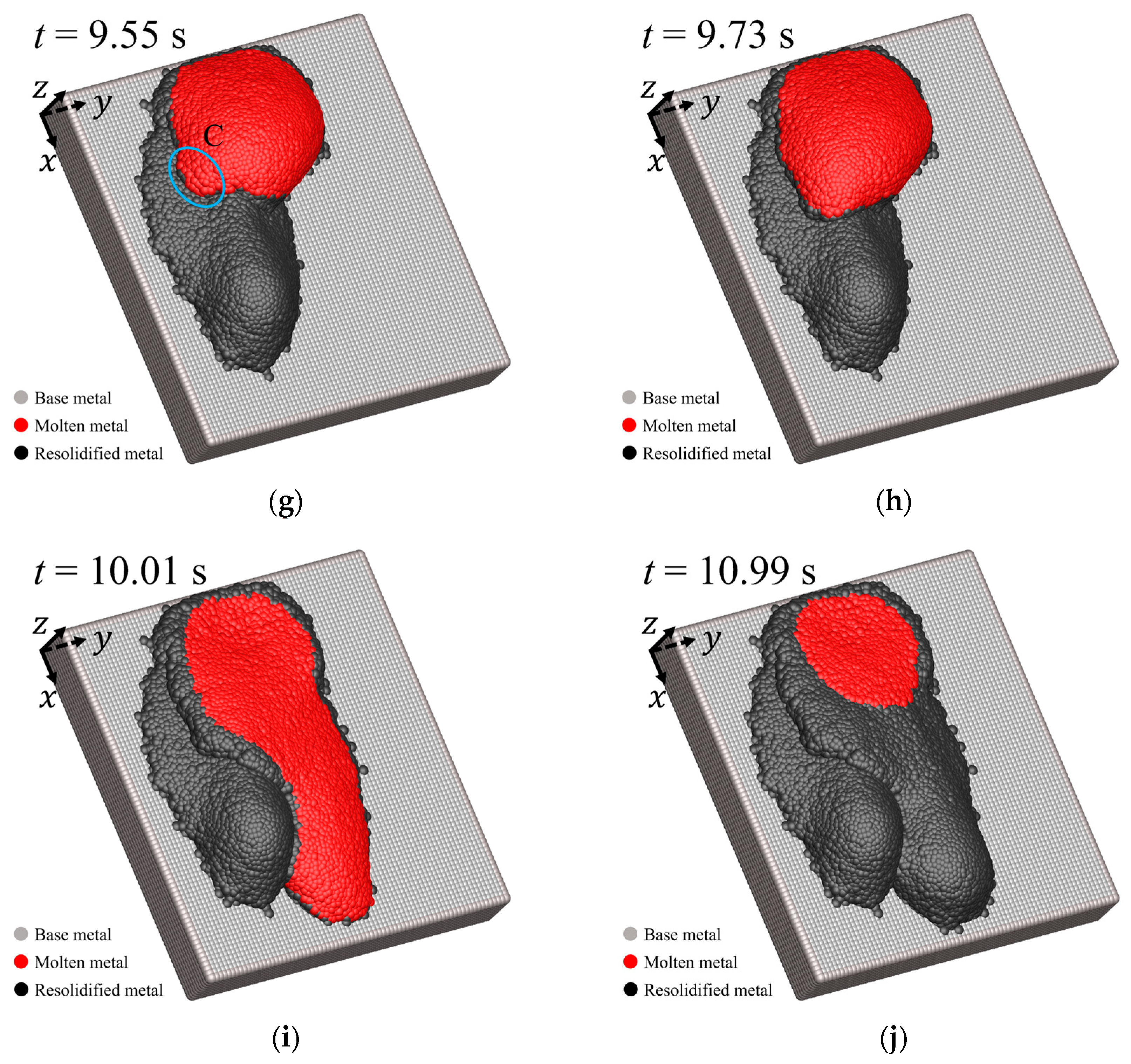
Figure 5 shows snapshots of a bird’s-eye view of the simulation results. In Figure 5, gray, red, and black particles indicate the base metal, the molten metal, and the resolidified molten metal, respectively.

As shown in Figure 5a, the base metal surface begins to melt because it receives sufficient heat energy from the heat source. The molten metal flows slowly in the $x$-direction under gravity, and a molten pool is formed (Figure 5b). The molten metal accumulates due to being dammed up in the $x$-direction while spreading in the $y$-direction (Figure 5c). After $t=5.74$ s, as shown in Figure 5d, the accumulated molten metal overflows greatly in the $x$-direction. The outer edge of the flow is solidified, and a levee-like structure is formed, as shown in part A in Figure 5d. Moreover, the tip of the flow becomes rounded, which is a toe-like shape, as shown in part B in this figure. At $t=7.08$ s, the flowed molten metal is cooled and solidified entirely, as shown in Figure 5e. The solidified tip is rounded and raised up.

Thereafter, the volume of the molten pool increases again through a continuous supply of molten metal (Figure 5f). At $t=9.55$ s, when the volume of the molten pool increases sufficiently, the molten metal begins to flow in the $x$-direction as shown in part C in Figure 5g. However, this overflow is held back, and the volume of the molten pool increases because the edges of the flow are quickly cooled and solidified at the solid–liquid interfaces (Figure 5h). After the molten metal accumulates sufficiently again, the molten metal overflows greatly in the $x$-direction again, as shown in Figure 5i. The molten metal flows on the resolidified metal, which flowed down first. At $t=10.99$ s, the second molten metal flow is cooled and solidified entirely, as shown in Figure 5j.

3.2. Discussion of the Formation Process of Structures Unique to Lava Flow

3.2.1. Levee-like Structure

Figure 6a shows the velocity in $x$-direction $u_x$, and Figure 6b, temperature distributions at $t=5.97$ s during the first flow. Figure 7a shows the velocity $u_x$, and Figure 7b, temperature distributions at $t=10.01$ s during the second flow. In the temperature distributions, gray particles indicate that their temperature is lower than the solidification point. As shown in Figure 6 and Figure 7, the outer edges are solidified and stationary because their temperatures become lower than the solidification point. On the other hand, the inside flows as a liquid phase because its temperature is still higher than the solidification point.

Figure 8 shows cross-sections at $x=18.0$ mm and at $t=5.97$ s. Only the particles located in 18.0 mm $\le x\le$ 20.0 mm are visualized. As shown in Figure 8a–c, the edges and bottom of the flow are cooled, solidified, and stationary. On the other hand, the top is still hot and flows. The solidified regions at the sides increase more in the $z$-direction than on the inside. Therefore, the levee-like structure is formed. This is a similar structure to that shown in Figure 1.

Figure 9 shows cross-sections at $x=20.0$ mm and at $t=10.01$ s. Only the particles located in 20.0 mm $\le x\le$ 22.0 mm are visualized. Line D–E traces the shape of the base metal and the resolidified metal, which flowed first. This line is used to distinguish the second flow from the first flow. The second molten metal flows on the base metal and the resolidified area of the first flow. During the second flow, the low-temperature solidified area increases from the solid–liquid interfaces indicated by the line D–E, as shown in Figure 9a–c. On the other hand, the molten metal away from the interfaces flows because its temperature is still higher than the solidification point. Therefore, the simulation considering the topographical change in the surface due to the solidification of the molten metal was successful.

Therefore, the present method is applicable to simulating lava levees and the accretion of the topography affecting the flow direction.

3.2.2. Shape of Tip

The tip shape of the flowing molten metal was rounded in this simulation, as shown in Figure 5d. This result was compared with that of an actual lava flow. Schott [37] photographed the tip shape of a lava flow at Mt. Kilauea. The tip shape in this simulation was similar to the toe-like shape of the actual lava tip. The solidified tip shape becomes rounded and raised up in this simulation, as shown in Figure 5e. This was similar to the shape observed at the solidified tip of the lava photographed by Hon et al. at Mt. Kilauea (See Figure 2c in Ref. [4]). The solidification areas overlap in this simulation, as shown in Figure 5j. This was also similar to the overlapping of solidified lava as shown in the photo by Hon et al. Therefore, the tendencies of the shape observed in this simulation show good agreement with the actual lava.

4. Conclusions

The eventual goal of this study was to simulate and clarify specific lava flow phenomena such as lava levees and lava overlapping in order to improve the prediction accuracy of inflow areas. As the first step, this study aimed to verify the feasibility of simulating lava flows with solidification. For simplicity, the lava was modeled with molten metal, with physical properties that were easily obtained, and treated as Newtonian fluid with constant viscosity, and it flowed down on a tilted surface. The conclusions of this study are summarized as follows:

• The levee-like shape was formed during the molten metal flowing down in this simulation. The outer edge of the flow was solidified and stationary due to its high cooling rate. On the other hand, the inside flowed as a liquid phase due to its low cooling rate. These flows resulted in formations that were qualitatively similar to the formations of lava levees in actual lava;
• The tip of the flow became rounded in this simulation. It was similar to the toe-like shape at the tip of lava. The tip became rounded and raised up after solidification. This was similar to the solidified tip of lava. It was also successfully simulated that molten metal flows on a surface that changes topographically due to the solidification of the molten metal.

As stated above, the computational model developed in this study using the SPH method is applicable to simulating lava levees, the influence of accretion, and the flow at the tip of lava. This study conducted only qualitative comparisons of the phenomena in this simulation with those in actual lava. However, the computational scheme used in this study has already made some achievements in simulating molten metal flow under welding conditions. For example, a previous study [31] simulated bead formation under arc welding, which is a similar phenomenon to the subject of this study. In the study, the simulation results were compared with experimental results. Quantitative agreement was obtained for bead shape and size. This indicates that our scheme is sufficiently reliable. In order to realize more accurate predictions, it will be necessary to conduct quantitative comparisons. To solve this problem, an experimental system is being constructed. This computational model is simpler than the model of Hérault et al. [13] and can be used to design the experimental system on a lab scale, which will be useful for future quantitative evaluations. In the system, lava flows will be modeled using molten metal flows during an arc welding process. It will be different from previous experiments in that it will allow the consideration of oxidation on the surface of lava. Moreover, lava was treated as a Newtonian fluid for a simplified model in this study. As discussed in Section 1, previous studies [13,18,19,20,21,22] have applied the SPH method to non-Newtonian fluids. In future work, it is also necessary to consider the non-Newtonian behavior of lava.

References

- Gregg, T.K.P.; Fink, J.H. A laboratory investigation into the effects of slope on lava flow morphology. J. Volcanol. Geotherm. Res. 2000, 96, 145–159. [Google Scholar] [CrossRef]
- Miyamoto, H.; Crown, D.A. A simplified two-component model for the lateral growth of pahoehoe lobes. J. Volcanol. Geotherm. Res. 2006, 157, 331–342. [Google Scholar] [CrossRef]
- Bokharaeian, M.; Novák, L.; Csámer, Á. Rheological study of lava flow analog mixtures. Acta Geodyn. Geomater. 2023, 20, 11–18. [Google Scholar] [CrossRef]
- Hon, K.; Kauahikaua, J.; Denlinger, R.; Mackay, K. Emplacement and inflation of pahoehoe sheet flows: Observations and measurements of active lava flows on Kilauea volcano, Hawaii. Geol. Soc. Am. Bull. 1994, 106, 351–370. [Google Scholar] [CrossRef]
- Quareni, F.; Tallarico, A.; Dragoni, M. Modeling of the steady-state temperature field in lava flow levées. J. Volcanol. Geotherm. Res. 2004, 132, 241–251. [Google Scholar] [CrossRef]
- Tsepelev, I.; Ismail-Zadeh, A.; Melnik, O.; Korotkii, A. Numerical modeling of fluid flow with rafts: An application to lava flows. J. Geodyn. 2016, 97, 31–41. [Google Scholar] [CrossRef]
- Starodubtsev, I.; Vasev, P.; Starodubtseva, Y.; Tsepelev, I. Numerical simulation and visualization of lava flows. Sci. Vis. 2022, 14, 66–76. [Google Scholar] [CrossRef]
- Tsepelev, I.; Ismail-Zadeh, A.; Starodubtseva, Y.; Korotkii, A.; Melnik, O. Crust development inferred from numerical models of lava flow and its surface thermal measurements. Ann. Geophys. 2019, 62, VO226. [Google Scholar]
- Starodubtsev, I.S.; Starodubtseva, Y.V.; Tsepelev, I.A.; Ismail-Zadeh, A.T. Three-dimensional numerical modeling of lava dynamics using the smoothed particle hydrodynamics method. J. Volcanol. Seismol. 2023, 17, 175–186. [Google Scholar] [CrossRef]
- Zago, V.; Bilotta, G.; Cappello, A.; Dalrymple, R.A.; Fortuna, L.; Ganci, G.; Hérault, A.; Del Negro, C. Simulating complex fluids with smoothed particle hydrodynamics. Ann. Geophys. 2017, 60, 669–679. [Google Scholar] [CrossRef]
- Zago, V.; Bilotta, G.; Cappello, A.; Dalrymple, R.A.; Fortuna, L.; Ganci, G.; Hérault, A.; Del Negro, C. Preliminary validation of lava benchmark tests on the GPUSPH particle engine. Ann. Geophys. 2018, 62, 224–236. [Google Scholar] [CrossRef]
- Zago, V.; Bilotta, G.; Hérault, A.; Dalrymple, R.A.; Fortuna, L.; Cappello, A.; Ganci, G.; Del Negro, C. Semi-implicit 3D SPH on GPU for lava flows. J. Comput. Phys. 2018, 375, 854–870. [Google Scholar] [CrossRef]
- Hérault, A.; Bilotta, G.; Vicari, A.; Rustico, E.; Del Negro, C. Numerical simulation of lava flow using a GPU SPH model. Ann. Geophys. 2011, 54, 600–620. [Google Scholar]
- Bašić, M.; Blagojević, B.; Peng, C.; Bašić, J. Lagrangian differencing dynamics for time-independent non-Newtonian materials. Materials 2021, 14, 6210. [Google Scholar] [CrossRef]
- Peshkov, I.; Dumbser, M.; Boscheri, W.; Romenski, E.; Chiocchetti, S.; Ioriatti, M. Simulation of non-Newtonian viscoplastic flows with a unified first order hyperbolic model and a structure-preserving semi-implicit scheme. Comput. Fluids 2021, 224, 104963. [Google Scholar] [CrossRef]
- Peng, C.; Bašić, M.; Blagojević, B.; Bašić, J.; Wu, W. A Lagrangian differencing dynamics method for granular flow modeling. Comput. Geotech. 2021, 137, 104297. [Google Scholar] [CrossRef]
- Castillo-Sánchez, H.A.; de Souza, L.F.; Castelo, A. Numerical simulation of rheological models for complex fluids using hierarchical grids. Polymers 2022, 14, 4958. [Google Scholar] [CrossRef] [PubMed]
- Shao, S.; Lo, E.Y.M. Incompressible SPH method for simulating Newtonian and non-Newtonian flows with a free surface. Adv. Water Resour. 2003, 26, 787–800. [Google Scholar] [CrossRef]
- Laigle, D.; Lachamp, P.; Naaim, M. SPH-based numerical investigation of mudflow and other complex fluid flow interactions with structures. Comput. Geosci. 2007, 11, 297–306. [Google Scholar] [CrossRef]
- Pan, W.; Tartakovsky, A.M.; Monaghan, J.J. Smoothed particle hydrodynamics non-Newtonian model for ice-sheet and ice-shelf dynamics. J. Comput. Phys. 2013, 242, 828–842. [Google Scholar] [CrossRef]
- Bilotta, G.; Zago, V.; Centorrino, V.; Dalrymple, R.A.; Hérault, A.; Del Negro, C.; Saikali, E. A numerically robust, parallel-friendly variant of BiCGSTAB for the semi-implicit integration of the viscous term in smoothed particle hydrodynamics. J. Comput. Phys. 2022, 466, 111413. [Google Scholar] [CrossRef]
- Shi, H.; Huang, Y. A GPU-based δ-plus-SPH model for non-Newtonian multiphase flows. Water 2022, 14, 1734. [Google Scholar] [CrossRef]
- Lan, Y.; Zhang, Y.; Tian, W.; Su, G.H.; Qiu, S. An enhanced implicit viscosity ISPH method for simulating free-surface flow coupled with solid-liquid phase change. J. Comput. Phys. 2023, 474, 111809. [Google Scholar] [CrossRef]
- Dingwell, D.B.; Webb, S.L. Structural relaxation in silicate melts and non-Newtonian melt rheology in geologic processes. Phys. Chem. Miner. 1989, 16, 508–516. [Google Scholar] [CrossRef]
- Lejeune, A.; Richet, P. Rheology of crystal-bearing silicate melts: An experimental study at high viscosities. J. Geophys. Res. 1995, 100, 4215–4229. [Google Scholar] [CrossRef]
- Monaghan, J.J. Smoothed particle hydrodynamics. Annu. Rev. Astron. Astrophys. 1992, 30, 543–574. [Google Scholar] [CrossRef]
- Koshizuka, S.; Oka, Y. Moving-particle semi-implicit method for fragmentation of incompressible fluid. Nucl. Sci. Eng. 1996, 123, 421–434. [Google Scholar] [CrossRef]
- Ito, M.; Izawa, S.; Fukunishi, Y.; Shigeta, M. Numerical simulation of a weld pool formation in a TIG welding using an incompressible SPH method. Q. J. Jpn. Weld. Soc. 2014, 32, 213–222. (In Japanese) [Google Scholar] [CrossRef]
- Shigeta, M.; Watanabe, T.; Izawa, S.; Fukunishi, Y. Incompressible SPH simulation of double-diffusive convection phenomena. Int. J. Emerg. Multidiscip. Fluid Sci. 2009, 1, 1–18. [Google Scholar] [CrossRef]
- Ito, M.; Nishio, Y.; Izawa, S.; Fukunishi, Y.; Shigeta, M. Numerical simulation of joining process in a TIG welding system using incompressible SPH method. Q. J. Jpn. Weld. Soc. 2015, 33, 34s–38s. [Google Scholar] [CrossRef]
- Komen, H.; Shigeta, M.; Tanaka, M. Numerical simulation of molten metal droplet transfer and weld pool convection during gas metal arc welding using incompressible smoothed particle hydrodynamics method. Int. J. Heat Mass Transf. 2018, 121, 978–985. [Google Scholar] [CrossRef]
- Tsujimura, Y. Gas Metal arc Yousetsu ni okeru Kinzokujouki wo Tomonau arc Genshou to sono Netsugentokusei ni Kansuru Kenkyu. Ph.D. Thesis, Osaka University, Osaka, Japan, 2012. (In Japanese). [Google Scholar]
- Komen, H.; Matsui, S.; Konishi, K.; Shigeta, M.; Tanaka, M.; Kamo, T. Modeling of submerged arc welding phenomena and experimental study of the heat source characteristics. Q. J. Jpn. Weld. Soc. 2017, 35, 93–101. (In Japanese) [Google Scholar] [CrossRef]
- Sahoo, P.; Debroy, T.; McNallan, M.J. Surface tension of binary metal—Surface active solute systems under conditions relevant to welding metallurgy. Metall. Trans. B 1988, 19, 483–491. [Google Scholar] [CrossRef]
- Komen, H.; Shigeta, M.; Tanaka, M.; Nakatani, M.; Abe, Y. Numerical simulation of slag forming process during submerged arc welding using DEM-ISPH hybrid method. Weld. World 2018, 62, 1323–1330. [Google Scholar] [CrossRef]
- Fukazawa, T.; Tanaka, K.; Komen, H.; Shigeta, M.; Tanaka, M.; Murphy, A.B. Numerical investigation for dominant factors in slag transfer and deposition process during metal active gas welding using incompressible smoothed particle hydrodynamics method. Q. J. Jpn. Weld. Soc. 2021, 39, 277–290. [Google Scholar] [CrossRef]
- Hawaiian Regional Geology. Available online: https://www.flickr.com/photos/rschott/310299013/in/photostream/ (accessed on 15 April 2024).
Figure 1.
Schematic of cross-section of lava flow.
Figure 2.
Computational domain.
Figure 3.
The temperature distribution of gas at [32].
Figure 4.
The heat input distribution for generating molten metal, which is expressed as ion recombination under arc plasma conditions [31].
Figure 5.
Flow and solidification processes of molten metal with time evolution: (a) at s; (b) at s; (c) at s; (d) at s; (e) at s; (f) at s; (g) at s; (h) at s; (i) at s; (j) at s.
Figure 6.
Molten metal flow at s: (a) -directional velocity distribution; (b) temperature distribution.
Figure 7.
Figure 8.
Cross-sections at mm and s: (a) phase of particles; (b) -directional velocity distribution; (c) temperature distribution.
Figure 9.