Entropy-Based Method of Choosing the Decomposition Level in Wavelet Threshold De-noising
Abstract
:1. Introduction
2. The Proposed Method of Choosing the Decomposition Level
2.1. Wavelet Threshold De-noising
2.2. Autocorrelations and Energy Distributions of Noises
| Type | Expression | Parameters |
|---|---|---|
| Normal | μ, σ | |
| Lognormal | μy, σy | |
| Pearson-III | α, β, a0 |

| Type | Index | Decomposition level (DL) | ||||||||
|---|---|---|---|---|---|---|---|---|---|---|
| 1 | 2 | 3 | 4 | 5 | 6 | 7 | 8 | 9 | ||
| Normal | R1 | −0.611 | 0.331 | 0.806 | 0.948 | 0.987 | 0.995 | 0.997 | 0.999 | 0.999 |
| E | 499.59 | 249.87 | 125.29 | 62.64 | 30.95 | 17.30 | 12.21 | 7.24 | 5.86 | |
| Lognormal | R1 | −0.612 | 0.332 | 0.806 | 0.948 | 0.987 | 0.996 | 0.998 | 0.999 | 0.999 |
| E | 499.50 | 249.42 | 125.15 | 62.70 | 30.91 | 17.24 | 11.94 | 7.09 | 5.70 | |
| Pearson-III | R1 | −0.611 | 0.331 | 0.806 | 0.948 | 0.987 | 0.996 | 0.997 | 0.999 | 0.999 |
| E | 499.45 | 250.21 | 124.89 | 62.61 | 30.97 | 17.44 | 12.14 | 7.32 | 5.83 | |

2.3. The Method Proposed
- (1)
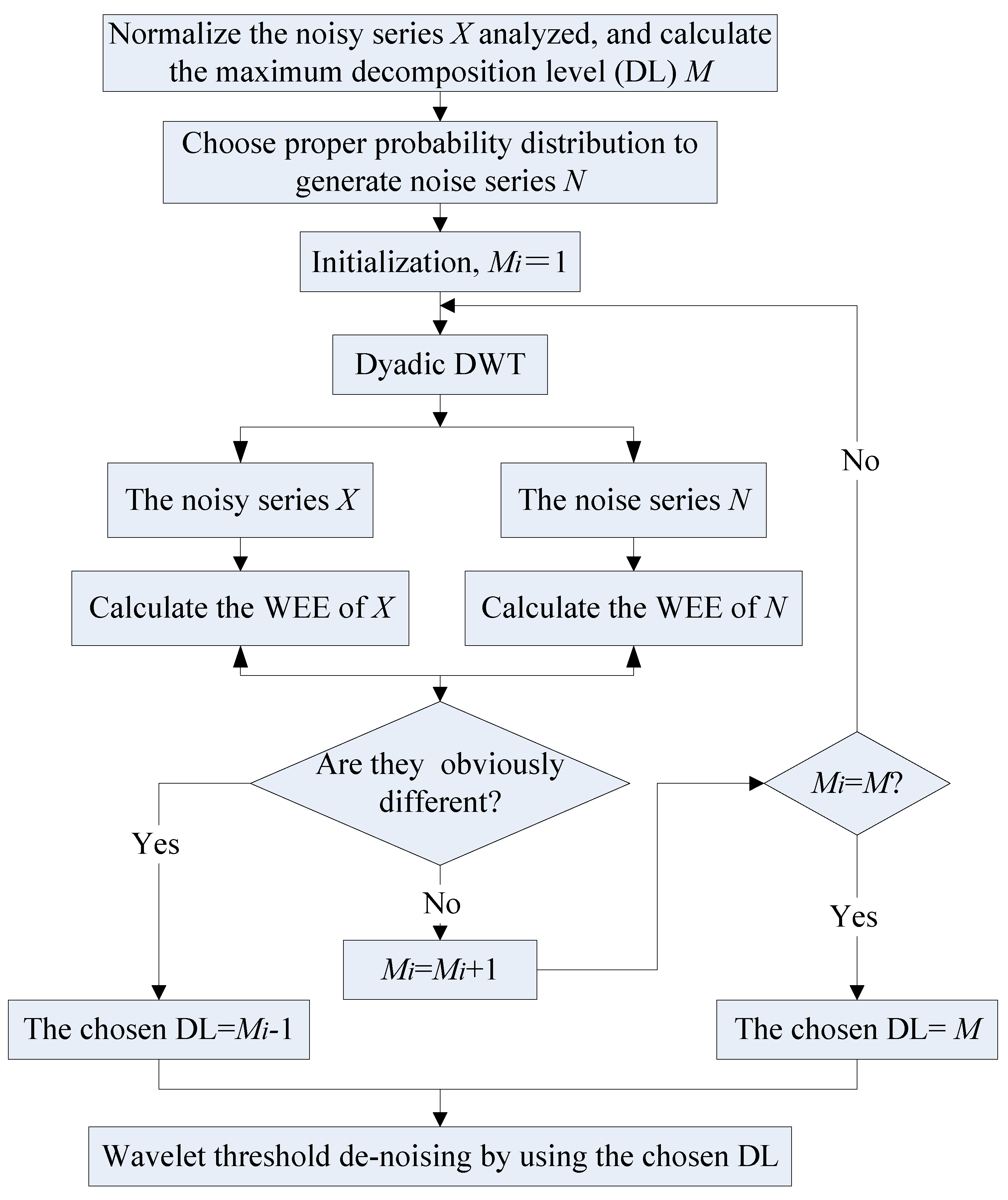
- For the noisy series X analyzed, we first calculate the theoretical maximum M of DL by Equation (2), and normalize it by Equation (5):in which and are the mean and standard deviation of X, respectively.
- (2)
- Then, we apply dyadic DWT to X by using each value of the DLs from 1 to M, and calculate the values of WEE by Equation (4), based on which we obtain the WEE curve of X.
- (3)
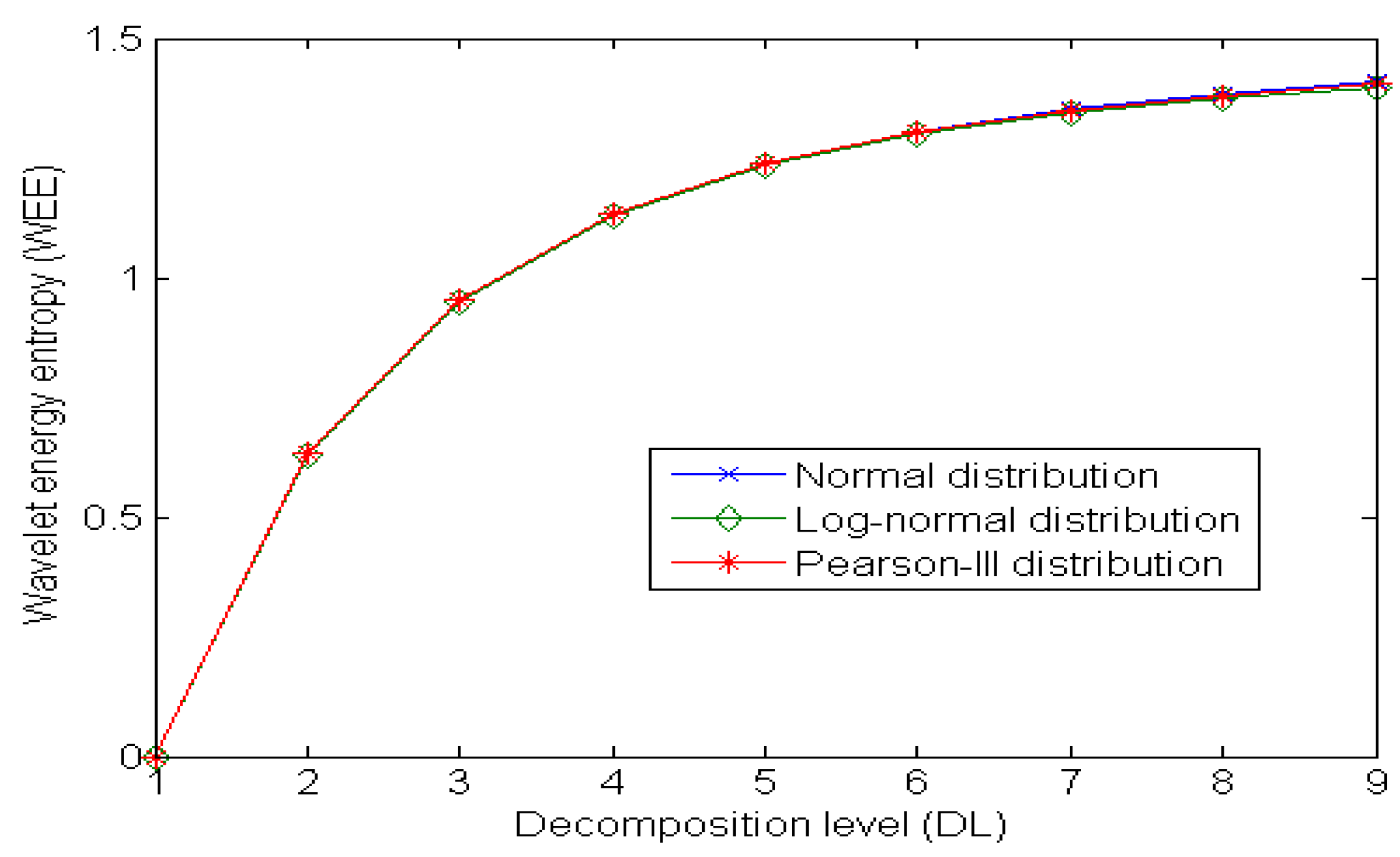
- According to the practical situations and experiences, we choose an appropriate probability distribution to generate “normalized” noise series with the same length as that of X. Then we determine the WEE curve of noise by doing Monte-Carlo tests.
- (4)
- Finally, we compare the values of WEE of the noisy series X with those of noise with the increasing of DLs. Once the value of WEE of X is obviously different from that of noise under certain DL*, the best DL can be chosen as DL* less 1. Besides, the differential coefficient of WEE in Equation (6) can be used together to compare the WEEs of noisy series X and noise, because it is an extreme value under the DL* and can reflect their difference more clearly;where D(j) is the differential coefficient of WEE under the DL j, d(∙) means the derivation calculus.

3. Case Studies
3.1. Synthetic Series Analysis


| Series | Index | Real value | Decomposition level (DL) | ||||||||
|---|---|---|---|---|---|---|---|---|---|---|---|
| 1 | 2 | 3 | 4 | 5 | 6 | 7 | 8 | 9 | |||
| SS1 | SNR | -9.562 | 4.844 | -2.121 | -5.543 | -7.466 | -8.310 | -9.383 | -9.581 | -9.530 | -9.545 |
| MSE | 0.469 | 0.236 | 0.121 | 0.065 | 0.040 | 0.013 | 0.005 | 0.004 | 0.010 | ||
| Rxy | 0.665 | 0.782 | 0.870 | 0.922 | 0.949 | 0.983 | 0.993 | 0.995 | 0.987 | ||
| SS2 | SNR | -4.012 | 7.054 | 0.954 | -1.833 | -3.983 | -18.58 | -19.18 | -19.67 | -25.38 | -29.27 |
| MSE | 1.708 | 0.839 | 0.417 | 0.387 | 1.500 | 1.481 | 1.458 | 1.59 | 1.611 | ||
| Rxy | 0.760 | 0.858 | 0.921 | 0.921 | 0.640 | 0.650 | 0.661 | 0.660 | 0.706 | ||
| SS3 | SNR | -3.365 | 7.867 | 1.811 | -1.048 | -1.792 | -4.525 | -10.46 | -17.82 | -19.45 | -19.53 |
| MSE | 0.305 | 0.146 | 0.067 | 0.046 | 0.074 | 0.158 | 0.191 | 0.211 | 0.224 | ||
| Rxy | 0.775 | 0.871 | 0.934 | 0.953 | 0.918 | 0.817 | 0.817 | 0.794 | 0.768 | ||


| Series | Decomposition level (DL) | |||||||||
|---|---|---|---|---|---|---|---|---|---|---|
| 1 | 2 | 3 | 4 | 5 | 6 | 7 | 8 | 9 | ||
| SS1 | -0.646 | 0.326 | 0.804 | 0.940 | 0.990 | 0.998 | 0.998 | 0.996 | 1.000 | |
| SS2 | -0.579 | 0.326 | 0.810 | 0.949 | 0.990 | 0.996 | 0.999 | 0.999 | 0.998 | |
| SS3 | -0.642 | 0.341 | 0.814 | 0.937 | 0.987 | 0.994 | 0.996 | 0.999 | 0.998 | |
3.2. Observed Series Analysis


| Series | Decomposition level (DL) | ||||||
|---|---|---|---|---|---|---|---|
| 1 | 2 | 3 | 4 | 5 | 6 | 7 | |
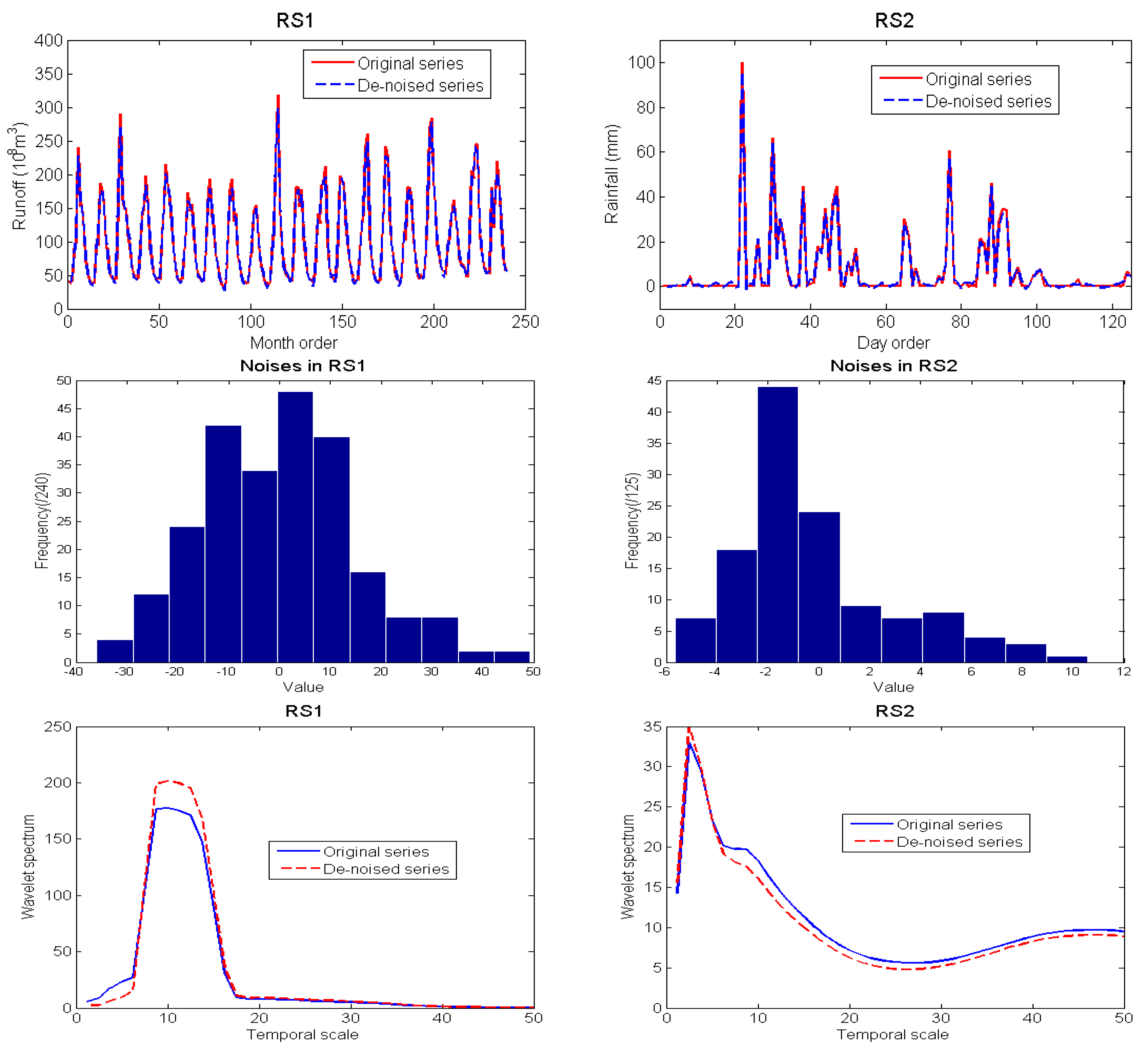
| RS1 | 30.904 | 26.768 | 20.049 | 18.200 | 17.297 | 16.705 | 16.285 |
| RS2 | 30.908 | 50.205 | 48.944 | 48.707 | 48.622 | 48.550 | |
| Series | Decomposition level (DL) | ||||||
|---|---|---|---|---|---|---|---|
| 1 | 2 | 3 | 4 | 5 | 6 | 7 | |
| RS1 | -0.562 | 0.431 | 0.856 | 0.962 | 0.980 | 0.995 | 0.999 |
| RS2 | -0.567 | 0.424 | 0.844 | 0.951 | 0.990 | 0.986 | |
4. Conclusions
Acknowledgements
References
- Kuczera, G. Uncorrelated measurement error in flood frequency inference. Water Resour. Res. 1992, 28, 183–188. [Google Scholar] [CrossRef]
- Hrachowitz, M.; Soulsby, C.; Tetzlaff, D.; Dawson, J.J.C.; Dunn, S.M.; Malcolm, I.A. Using long-term data sets to understand transit times in contrasting headwater catchments. J. Hydrol. 2009, 367, 237–248. [Google Scholar] [CrossRef]
- Wang, D.; Singh, V.P.; Zhu, Y.S.; Wu, J.C. Stochastic observation error and uncertainty in water quality evaluation. Adv. Water Resour. 2009, 32, 1526–1534. [Google Scholar] [CrossRef]
- Sang, Y.F.; Wang, D.; Wu, J.C.; Zhu, Q.P.; Wang, L. The relation between periods’ identification and noises in hydrologic series data. J. Hydrol. 2009, 368, 165–177. [Google Scholar] [CrossRef]
- Donoho, D.H. De-noising by soft-thresholding. IEEE Trans. Inform. Theory 1995, 41, 613–617. [Google Scholar] [CrossRef]
- Natarajan, B.K. Filtering random noise from deterministic signals via data compression. IEEE Trans. Signal Process. 1995, 43, 2595–2605. [Google Scholar]
- Kazama, M.; Tohyama, M. Estimation of speech components by AFC analysis in a noisy environment. J. Sound Vib. 2001, 241, 41–52. [Google Scholar] [CrossRef]
- Elshorbagy, A.; Simonovic, S.P.; Panu, U.S. Noise reduction in chaotic hydrologic time series: facts and doubts. J. Hydrol. 2002, 256, 147–165. [Google Scholar] [CrossRef]
- Torrence, C.; Compo, G.P. A practical guide to wavelet analysis. Bull. Amer. Meteorol. Soc. 1998, 79, 61–78. [Google Scholar] [CrossRef]
- Percival, D.B.; Walden, A.T. Wavelet Methods for Time Series Analysis; Cambridge University Press: Cambridge, UK, 2000. [Google Scholar]
- Jansen, M.; Bultheel, A. Asymptotic behavior of the minimum mean squared error threshold for noisy wavelet coefficients of piecewise smooth signals. IEEE Trans. Signal Process. 2001, 49, 1113–1118. [Google Scholar] [CrossRef]
- Jansen, M. Minimum risk thresholds for data with heavy noise. IEEE Signal Process. Lett. 2006, 13, 296–299. [Google Scholar] [CrossRef]
- Sang, Y.F.; Wang, D.; Wu, J.C.; Zhu, Q.P.; Wang, L. Entropy-based wavelet de-noising method for time series analysis. Entropy 2009, 1, 1123–1147. [Google Scholar] [CrossRef]
- Coifman, R.; Wickerhauster, M.V. Entropy based algorithms for best basis selection. IEEE Trans. Inform. Theor. 1992, 38, 713–718. [Google Scholar] [CrossRef]
- Berger, J.; Coifman, R.D.; Goldberg, M.J. Removing noise from music using local trigonometric bases and wavelet packets. J. Audio Eng. Soc. 1994, 42, 808–818. [Google Scholar]
- Lou, H.W.; Hu, G.R. An approach based on simplified KLT and wavelet transform for enhancing speech degraded by non-stationary wideband noise. J. Sound Vib. 2003, 268, 717–729. [Google Scholar]
- Dimoulas, C.; Kalliris, G.; Papanikolaou, G.; Kalampakas, A. Novel wavelet domain Wiener filtering de-noising techniques: application to bowel sounds captured by means of abdominal surface vibrations. Biomed. Signal Process. Contr. 2006, 1, 177–218. [Google Scholar] [CrossRef]
- Chui, C.K. An Introduction to Wavelets, Vol. 1 (Wavelet Analysis and Its Applications); Academic Press: Boston, MA, USA, 1992. [Google Scholar]
- Bruni, V.; Vitulano, D. Wavelet-based signal de-noising via simple singularities approximation. Signal Process. 2006, 86, 859–876. [Google Scholar] [CrossRef]
- Chanerley, A.A.; Alexander, N.A. Correcting data from an unknown accelerometer using recursive least squares and wavelet de-noising. Comput. Struct. 2007, 85, 1679–1692. [Google Scholar] [CrossRef]
- Box, G.E.P.; Jenkins, G.M.; Reinsel, G.C. Time Series Analysis, Forecasting and Control; Prentice-Hall: Saddle River, NJ, USA, 1994. [Google Scholar]
- Jaynes, E.T. Information theory and statistical mechanics. Phys. Rev. 1957, 106, 620–630. [Google Scholar] [CrossRef]
- Labat, D. Recent advances in wavelet analyses: Part 1. A review of concepts. J. Hydrol. 2005, 314, 275–288. [Google Scholar] [CrossRef]
- Wang, W.S.; Ding, J.; Li, Y.Q. Hydrology Wavelet Analysis (in Chinese); Chemical Industry Press: Beijing, China, 2005. [Google Scholar]
- Sang, Y.F.; Wu, J.C.; Wang, D.; Ling, C.P. New Model of Groundwater Simulation and Prediction Based on Wavelet De-noising. In Proceedings of 7th International Conference on Calibration and Reliability in Groundwater Modeling, Wuhan, China, September 2009; pp. 55–58.
© 2010 by the authors; licensee MDPI, Basel, Switzerland. This article is an open access article distributed under the terms and conditions of the Creative Commons Attribution license (http://creativecommons.org/licenses/by/3.0/).
Share and Cite
Sang, Y.-F.; Wang, D.; Wu, J.-C. Entropy-Based Method of Choosing the Decomposition Level in Wavelet Threshold De-noising. Entropy 2010, 12, 1499-1513. https://doi.org/10.3390/e12061499
Sang Y-F, Wang D, Wu J-C. Entropy-Based Method of Choosing the Decomposition Level in Wavelet Threshold De-noising. Entropy. 2010; 12(6):1499-1513. https://doi.org/10.3390/e12061499
Chicago/Turabian StyleSang, Yan-Fang, Dong Wang, and Ji-Chun Wu. 2010. "Entropy-Based Method of Choosing the Decomposition Level in Wavelet Threshold De-noising" Entropy 12, no. 6: 1499-1513. https://doi.org/10.3390/e12061499
APA StyleSang, Y.-F., Wang, D., & Wu, J.-C. (2010). Entropy-Based Method of Choosing the Decomposition Level in Wavelet Threshold De-noising. Entropy, 12(6), 1499-1513. https://doi.org/10.3390/e12061499


