Abstract
We derive an algorithm to recursively determine the lap number (minimal number of monotonicity segments) of the iterates of twice differentiable l-modal map, enabling to numerically calculate the topological entropy of these maps. The algorithm is obtained by the min-max sequences—symbolic sequences that encode qualitative information about all the local extrema of iterated maps.
1. Introduction
Entropy is a ubiquitous tool in physics and mathematics. It measures randomness in dynamical systems, uncertainty in information theory and disorder in statistical mechanics.
Topological entropy was introduced in 1965 by Adler, Konheim and McAndrew [1] as an invariant of topological conjugacy for maps of the interval. Along with the Lyapunov exponent, topological entropy is one of the preferred indicators for complexity in topological dynamics. The numerical computation of topological entropy has been and remains an active topic of research, as witnessed by a number of relevant publications in the last decades.
Let I be a compact interval and be a continuous piecewise monotone map. Such a map is called l-modal if f has precisely l turning points (i.e., points in where f has a local extremum). Assume that f has local extrema at and that f is strictly monotone in each of the intervals
To such map one can assign a positive or negative shape which describes whether f is increasing or decreasing on its first lap . In proofs it is occasionally convenient to use the convention and . Sometimes the additional condition is also required (see for instance [2]); in this case we speak of boundary-anchored maps. We shall also consider boundary-anchored maps below but only as a special case, since the general algorithm for the topological entropy then simplifies quite a bit.
The itinerary of under f is the sequence defined as follows:
The itineraries of the critical points,
are called the kneading sequences(or invariants) of f.
Let denote the topological entropy of an l-modal map . Then [3,4],
where Var stands for the variation of , and is shorthand for the lap number of (i.e., the number of maximal monotonicity segments of ). There are relations similar to (1) and (2), involving the number of fixed points of (i.e., the number of periodic points of period n), or the length of the graph of .
The methods proposed in the literature to compute , use typically kneading sequences [5,6,7], approximating piecewise linear maps [8] and Markov maps [9], the Ruelle–Perron–Frobenius operator [10], or one of the expressions (1) and (2) [11,12]. Their virtues and shortcomings are also discussed in the literature. For instance, some are meant only for unimodal maps [5,7] or bimodal maps [6]. Others apply to not necessarily continuous piecewise monotone maps of the interval, however they are not efficient nor even accurate [8].
The method proposed here calculates the lap numbers , , and the topological entropy follows from (2). It applies to multimodal maps with or without boundary conditions. The main ingredient of this approach are the so-called min-max sequences—symbolic sequences that encode the coarse-grained information about the extrema of the maps , . It generalizes an approach for unimodal, boundary anchored maps, introduced in [13,14], further developed in [15], and extended for boundary free maps in [16].
The method proposed here is conceptually simple, is direct, is geometrical and is computationally efficient, calculating the lap numbers in a recursive way. The structure of the algorithm is the same for all l-modal maps, independently of the value of l. Regarding computing speed, we shall not provide any sharper bound than the convergence rate derivable on general grounds [12]. Nonetheless, numerical simulations confirm the excellent performance of the algorithm—except when , in which case the convergence is slow.
The rest of the paper is organized as follows. In Section 2 we introduce the min-max sequences of a map , where is the class of twice differentiable l-modal maps. This assumption simplifies the proofs but the results obtained in this paper apply to the class of continuous piecewise monotonous maps. In Section 3, we derive a number of technical lemmas, which are needed in the next two sections. Section 4 is devoted to clarify the connection between the min-max sequences of a map and the structure of its extrema, exploring the geometrical meaning of the min-max sequences. This connection leads in Section 5 to the main result of the paper, Theorem 5.3, which provides a recursive scheme for computing (hence ) with arbitrary precision. It turns out that the general scheme of Theorem 5.3 simplifies in some special cases, notably for boundary-anchored maps and for unimodal maps; these cases are separately discussed in Section 6. The paper concludes with the logical flow of the algorithm (Section 7), and a summary of numerical simulations with 2- and 3-modal maps (Section 8).
2. Geometry of the Itineraries: The Min-Max Sequences for l-Modal Maps
Henceforth we consider the class of twice differentiable l-modal maps. Since the results we obtain in Section 5 for the calculation of lap numbers and topological entropy do not depend on the shape of f, we shall assume throughout that the shape of f is positive, that is,
where [resp. ] denotes any with odd [resp. even], and , are meant to be the appropriate one-sided derivatives.
The chain rule for derivation applied to the nth iterate of f, written ( is the identity map),
implies trivially
which shows that are critical points of for every . From (5) we conclude also the following.
Lemma 2.1.
If , then the critical points of , , are the points such that for some and .
Therefore, the critical points of with are the pre-images of the critical points ,..., up to order .
Our next scope is a relation between the kneading sequences of and the structure of local extrema of . According to the assumption (3),
where .
The next lemma follows readily from (4) and
Lemma 2.2.
Let , and . Then:
- (a)
- If with i odd, then is a maximum. If with i even, then is a minimum.
- (b)
- If is a minimum, then
- (b)
- If is a maximum, then
For our purposes it will be sufficient to know which element of the partition the points , and belong to. This information can be conveniently codified by assigning to a signature defined as follows: For ,
Therefore there are only signatures, one for each element of . Note that if , , then
Otherwise, if , , then
The cases , or need no further comments. Thus, in a signature the +’s appear always left of the −’s, occasionally separated by a 0.
Two further tools will prove useful later on.
- We borrow from the real analysis a product ‘·’ among the symbols :
- If in , then , where here < stands for the lexicographical order of signatures induced by .
Suppose that , , has a maximum [resp. minimum] at some point . We say that is a maximum [resp. minimum] with signature if . Sometimes we also say that is a σ-maximum [resp. σ-minimum] with the obvious meaning.
To locate the extrema of in I up to the precision set by the partition , we introduce a new alphabet
where m stands for “minimum”, M stands for “maximum”, and the superscript σ is the pertaining signature, i.e., if is the minimum or maximum considered, then . Correspondingly we say that is an extremum of type [resp. ], or just that is a σ-minimum [resp. σ-maximum].
Next we define l sequences , , as follows:
The sequences are called the min-max sequences of , or MMSs for short. The geometric meaning of is clear: is a maximum (if ) or a minimum (if ) with signature .
By particularizing Lemma 2.2 to , , and , , we get the transition rules listed in Table 1.

Table 1.
Consecutive symbols in the MMS follow the above transition rules.
| → | ||
| → | ||
| → | ||
| → | ||
| → | ||
| → | ||
| → |
3. Auxiliary Lemmas
As stated before, the generic structure of a signature is
Therefore, when comparing component-wise two signatures, only three cases can happen: (i) all components coincide, (ii) they differ in a single component, or (iii) they differ in a number of consecutive components. Of course, case (ii) can be considered as a “degenerate” subcase of (iii), as we will do in the sequel.
Let and set,
In particular, . According to Lemma 2.1, contains and its preimages up to order . This same lemma implies that if is a critical point of , , then x is also a critical point of for . Hence, . It follows from Lemma 2.2 that all these critical points are local maxima or minima, but not inflexion points.
Furthermore, let [resp. ] be the leftmost [resp. rightmost] critical point of , i.e.,
for . Observe that and .
Lemma 3.1.
Let and , , be
- two consecutive critical points of ( if ), or
- and , or
- , and .
- (a)
- If for (, ) and otherwise, then there exist critical points ,..., of in . Furthermore, , , and has a maximum at if is even (hence is a -maximum in this case), while has a minimum at if is odd (hence is a -minimum in this case). Moreover, if , while if .
- (b)
- Otherwise (i.e., for ), there exist no critical points of in .
The geometrical interpretation of this lemma in the Cartesian plane is clear. If in (a), then the curve , , crosses transversally the “ith critical line” , and none of the other critical lines (if any) , . If , then this curve crosses transversally successive critical lines, namely, up to , and none of the remaining ones (if any). In (b) both and belong to the same interval , so does not cross any critical line when .
Proof.
(a) Suppose (the case follows analogously). By the monotonicity of in and the Mean Value Theorem, there exist exactly different points such that for . Then
and
Therefore,
because according to (6), is a maximum in the first case, and a minimum in the second.
The statement about the relative positions of , is obvious from the geometrical interpretation.
(b) This assertion is straightforward. ☐
Setting , in Lemma 3.1, we conclude the following results.
Lemma 3.2.
Let and .
- (a)
- If for (, ) and otherwise, then . Furthermore, if , then , and is a -maximum if is odd or a -minimum if is even. If , then , and is a -maximum if is even or a -minimum if is odd.
- (b)
- Otherwise (i.e., for ), holds. Furthermore,
- (b1)
- is a maximum if (i) is a maximum and , or (ii) is a minimum and ;
- (b2)
- is a minimum if (i) is a maximum and , or (ii) is a minimum and .
Proof.
(a) is a corollary of Lemma 3.1 (a). The first statement of (b) is a corollary of Lemma 3.1 (b).
As for (b1) and (b2),
because is a critical point of . Moreover,
Thus, and have the same sign if and only if (so as , see (3)). ☐
And setting , in Lemma 3.1, we derive the following results in a way similar to Lemma 3.2.
Lemma 3.3.
Let and .
- (a)
- If for (, ) and otherwise, then . Furthermore, if , then , and is a -maximum if is even or a -minimum if is odd. If , then , and is a -maximum if is odd or a -minimum if is even.
- (b)
- Otherwise (i.e., for ), holds. Furthermore,
- (b1)
- is a maximum if (i) is a maximum and , or (ii) is a minimum and ;
- (b2)
- is a minimum if (i) is a maximum and , or (ii) is a minimum and .
The results for boundary-anchored maps are simpler. Since we are assuming that has a positive shape, the boundary conditions of such a map read: for any l, and for l odd, or for l even. It follows , and or , respectively, for any . To prove the next two lemmas, the following weaker boundary conditions are sufficient, though:
- (BC1)
- , and
- (BC2)
- if l is odd, or if l is even,
Lemma 3.4.
Let be a quasi boundary-anchored map such that
- (H1)
- , and
- (H2)
- (l odd) or (l even).
- (a)
- , , and is a maximum.
- (b)
- (l odd) , , and is a maximum.
- (c)
- (l even) , , and is a minimum.
Proof.
(a) Suppose for all (BC1), and (H1). Then for . According to Lemma 3.2 (a) with , , and , we have and is a maximum. By induction it follows that and is a maximum for .
(b) Suppose l odd, for all (BC2), and (H2). Then for . According to Lemma 3.3 (a) with , , and , we have and (by H1) is a maximum. By induction it follows that and is a maximum for .
(c) Suppose l even, for all (BC2), and (H2). Then for . According to Lemma 3.3 (a) with , , and , we have and is a minimum. By induction it follows that and is a minimum for . ☐
Lastly, the next lemma is a kind of complementary result to Lemma 3.4.
Lemma 3.5.
Let be a quasi boundary-anchored map such that
- (H1)
- , and
- (H2)
- (l odd) or (l even).
- (a)
- , , and is a maximum.
- (b)
- (l odd) , , and is a maximum.
- (c)
- (l even) , , and is a minimum.
Proof.
(a) Suppose for all (BC1), and (H1). Then (i.e., ) for all , because f is assumed to be strictly increasing in [Equation (3)]. Therefore, for . According to Lemma 3.2 (b) with , we have , and is a maximum because is a maximum [Equation (6)] and . By induction it follows that and is a maximum for .
(b) Suppose l odd, for all (BC2), and (H2). Then for any , because f is assumed to be strictly increasing in and (H1). Therefore, for . According to Lemma 3.3 (b) with , we have , and is a maximum because is a maximum [Equation (6) with l odd] and . By induction it follows that and is a maximum for .
(c) Suppose l even, for all (BC2), and (H2). Then for any , because f is assumed to be strictly increasing in . Therefore, for . According to Lemma 3.3 (b) with , we have , and is a minimum because is a minimum [Equation (6) with l even] and ( odd). By induction it follows that and is a minimum for . ☐
4. Counting Laps
Given the kneading sequences of a map , it is possible to draw qualitatively the graph of for any . The procedure to be explained shortly is based on the geometrical meaning of the MMSs, Lemma 2.1, and the auxiliary lemmas 3.1–3.3; see Example 4.2 below for an illustration.
- (A)
- Fix and using the transition rules in Table 1, determine the first n terms of the min-max sequences , , from the seeds , if i is odd, and , if i is even. For the exposition it is convenient to introduce the notationActually, from and we shall only need their signatures. Remember that and .
- (B)
- Draw two perpendicular axes and divide the vertical axis into n rows corresponding, top to bottom, to the iterates , . The horizontal axis represents the interval . Enter along this axis the labels a, , ..., and b, and write column-wise below them, top to bottom, the sequences , ..., , and , respectively (see Table 2 and Table 3). These columns will be called the -, ..., -column, respectively. Leave ample space between these columns to insert further columns as we proceed with the present construction.
- (C)
- Proceed now row-wise, say left to right, starting with the row. We are going to compare pair-wise the signatures of neighboring symbols.
- (C1)
- Consider first the unimodal case (. If , then insert between the - and the -column, shifted one row downward (i.e., is on the -th row). If , then insert between the - and the -column, shifted again one row downward. Otherwise, no action is taken.
- (C2)
- Consider now the multimodal case (). If for (, ) and otherwise, then insert the MMSs , ..., between the - and the -column, shifted one row downward. Otherwise, no action is taken. Furthermore, if (i.e., is increasing in the lap ), then the MMSs , ..., are inserted in exactly that order. If (i.e., is decreasing in the lap ), then the MMSs , ..., are inserted in the reversed order: , ..., . Repeat this procedure with all remaining pairs of neighboring symbols on row .
- (D)
- Apply the procedure explained in (C) to the rows . At the end, row n exhibits the extrema of in .
Remark 4.1.
With regard to (C2) and (D), the order of and coincides with the order of and for any . In the case and , holds because we are assuming that f has a positive shape. Nonetheless we consider also the possibility in (C2) to explain the general procedure in further steps.
In order to bring clarity into the notation, we stick in the sequel to the above usage: n and the Greek letters (mostly as subindices, and belonging to or ) will refer to map iterations, while the Latin letters (mostly as upper indices, and belonging to ) will refer to the critical points.
Example 4.2.
The cubic polynomial
defines on a bimodal map with a local maximum at () and a local minimum at (). Figure 1 shows that
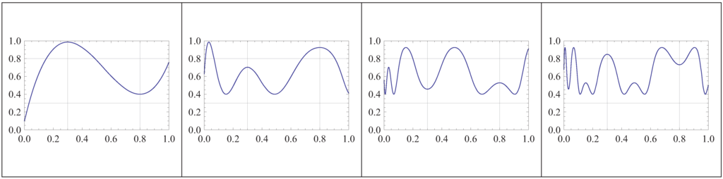
Figure 1.
Graphs of f, , , and for the bimodal map (15).
Figure 1.
Graphs of f, , , and for the bimodal map (15).
The first four components of both MMSs have been written on the corresponding column of Table 2 (for and Table 3 (for , respectively. The data and , , appear on the - and -column, respectively. The additional labels stand for the critical points of . The distribution of the critical points and values of , , will emerge as we apply the procedure (A)–(D) to this particular map. The information about the critical points comprises their number and relative position (or ordering) in the interval ; the corresponding critical values are located up to the precision set by the partition . The details are as follows.
- 1.
- Since , , and , we insert and , beginning on row , in the given order: at , at , with (Rule C2). There is only place for the first three components.
- 2.
- Since , and , we insert and shift at , .
- 3.
- To complete the first row, we observe that and , so no action is taken. This means that no column right of the -column will start on row . Note that the leftmost critical point of is , being a -maximum, and that the rightmost critical point of is , being also a -maximum.
- 4.
Table 2.
Extrema of , , for the map (15), in the interval .
| ν | ||||||||
| 1 | ||||||||
| 2 | ||||||||
| 3 | ||||||||
| 4 |
Table 3.
Extrema of , , for the map (15), in the interval .
| ν | |||||||||
| 1 | |||||||||
| 2 | |||||||||
| 3 | |||||||||
| 4 |
5. The Main Result
Given , let denote the lap number of , and the number of local extrema (or critical points) of , with . Since is continuous and piecewise monotone, the laps are separated by critical points, hence the relation,
holds. In particular,
since , the identity, is monotonically strictly increasing, and
Furthermore, let , , stand for the number of interior simple zeros of , , i.e., solutions of (), or (ii) solutions of , with , with for , and (). Geometrically is the number of transversal intersections in the Cartesian plane of the curve and the straight line , over the interval . Note that
for all i.
To streamline the notation in the forthcoming results, set
for . In particular,
Lemma 5.1.
Let . Then, for ,
Proof.
For , use the fact that equals the number of sign changes of . Then, Equation (22) follows from the relation . Note that the x’s with and are counted only once (by ), since they are not simple zeros of . ☐
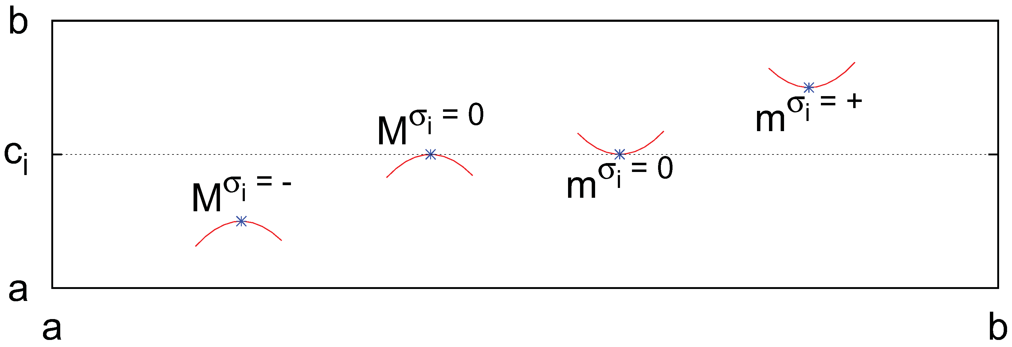
Consider fixed but otherwise arbitrary indices and . The following two observations are trivial: (i) the upper bound of corresponds to the case in which the graph of crosses the ith critical line on every lap; (ii) the row ν of the MM-table of contains alternating maxima and minima, i.e., alternating symbols and corresponding to the graph points, say, and , respectively. If , then the curve joining the corresponding extrema crosses the critical line . If, otherwise, , then one of the two symbols involved is necessarily a “bad” symbol, to wit: (i) with , so as the curve does not cross the ith critical line on the lap , or (ii) with , so as the curve does not cross either the ith critical line on the same lap. Call
the set of bad symbols or types with respect to the ith critical line. Moreover note that if a bad symbol appears on a column other than the - or -column, then the same conclusion concerning the zeros of applies to the two laps of left and right of corresponding extremum. And if a bad symbol appears on the - and/or -column, then there is no zero of in and/or .
Figure 2 illustrates the geometrical meaning of a bad symbol : The branches of the parabolic approximation to a local extrema whose type is a bad symbol point away from the critical line . It is easy to check that
For example, for
If we say that is a good symbol with respect to the ith critical line. Since there are symbols and symbols , the number of good symbols with respect to the ith critical line is .
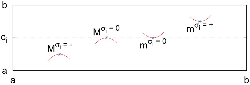
Figure 2.
Geometrical meaning of the bad symbols (25).
Figure 2.
Geometrical meaning of the bad symbols (25).
Therefore, the equality is only possible if the row ν in the MM-table of contains only good symbols with respect to the critical line . Indeed, we have just seen that each bad symbol on row ν subtracts two simple zeros (solutions of , ) from . But that condition is not sufficient. It could also happen that the leftmost extremum is of good type, but has no zero in the interval because , i.e., the graph points and are both above or both below the critical line . Of course, a similar consideration holds for the rightmost extremum and too.
All these facts can be encapsulated in the relation
where is the number of symbols from the bad set and
Before using the previous results to formulate a recursive procedure to calculate the lap number , we need to relate the symbols on the - and -columns to the critical values and .
Remember that in the construction of the MM-table of f, we may encounter two situations in the intervals (a similar discussion holds for the intervals ).
- (S1)
- If , for , and otherwise, then [Lemma 3.2 (a)], and we write down (if ) or (if ) on the -column, beginning at row ν. To address both possibilities in the present discussion, denote by the sequence on the -column (note if ).
- (S2)
- On the other hand, suppose for all , and (or if ). In this case [Lemma 3.2 (b)]. If again for all i, then . In general, if this happens τ consecutive times (i.e., for ), then (i) , and (ii) the leftmost extrema are of type , respectively (see Table 2).
In order to accommodate all these possibilities in the notation, will denote the -entry in the MM-table of f, i.e., the symbol on the row ν of the -column. Analogously, will designate the -entry in the MM-table of f. From (27), (S1) and (S2), it follows
where , , and for ,
with , and . Here [resp. ] are meant to be the smallest [resp. greatest] values of the index i for which the corresponding inequalities hold, and [resp. ] stands for a maximum [resp. minimum] of any signature. The functions , are recursively calculated as follows: , and for ,
Table 4.
Values of and for the bimodal map (15).
| ν | ||||||||
| 1 | 1 | 1 | 0 | 0 | 2 | 1 | 0 | 1 |
| 2 | 1 | 1 | 1 | 0 | 2 | 2 | 1 | 0 |
| 3 | 2 | 1 | 0 | 1 | 2 | 1 | 0 | 0 |
| 4 | 2 | 2 | 1 | 0 | 2 | 1 | 0 | 1 |
Let us understand the geometrical meaning of the values of, say, row in view of the MM-table of f, Table 2 and Table 3.
- and because the leftmost column beginning at or intersecting the row (the -column) has the symbol on row .
- because , i.e., it is a bad symbol with respect to the critical line (so the lack of a zero of in the interval is already accounted for in the term of Equation (26)). On the other hand, because , i.e., it is a good symbol with respect to the critical line but (see the second sign on row of the -column), so has no zero in the interval .
- and because the rightmost column beginning at or intersecting the row (i.e., the -column) has the symbol on row .
- because . On the other hand, because is a good symbol with respect to the critical line and, furthermore, (see the second sign on row of -column), so has one zero in the interval .
We can now derive the main result of this paper.
Theorem 5.3.
Let be the number of sequences that begin at row ν on the MM-table of f, and, as before, let be the number of symbols of on row ν. Then,
By Lemma 3.1, for . Since and (19), , we conclude that for as well. Upon substitution of this equality and Equation (26) into Equation (33), we obtain
Finally, use (24) to derive the expression (32). ☐
In view of (31), Equation (32) can be shortened to
In particular, , and , hence since for every k (19). Therefore
Example 5.4.
Table 5.
Lap numbers of the first four iterates of the map (15).
| ν | ||||||
| 1 | ∅ | 1 | 2 | 3 | 3 | |
| 2 | 0 | 4 | 4 | 6 | ||
| 3 | 0 | 5 | 5 | 10 | ||
| 4 | 0 | 10 | 10 | 15 |
Two comments are in order at this point.
First, the computation scheme (31) and (32) for the lap number only involves two ingredients: The first n symbols of the l MMSs of f, and the first n signatures of the itineraries of both endpoints.
Secondly, the number of summations in (31) and (32) for the computation of is . Moreover, this scheme is almost recursive. Indeed the value of is determined by the values of , , ..., along with the values of , which have to be calculated anew for each ν. Thus, in the particular case for all and , the algorithm is not only much simpler but fully recursive.
6. Special Cases
The next two lemmas provide sufficient conditions for all ’s and ’s in (32) to vanish. Remember that a map is called quasi boundary-anchored if it satisfies the boundary conditions (BC1) and (BC2) of Section 3. The most prominent instance of quasi boundary-anchored maps are the boundary-anchored ones.
Lemma 6.1.
Let be a quasi boundary-anchored map such that
- (H1)
- , and
- (H2)
- (l odd) or (l even).
Then , , , , and
for all , .
Proof.
From Lemma 3.4 (a)–(c) and their corresponding proofs, we conclude the following results.
(a) , , and
[see (25)] for all ,
(b) , , and
for all , , l odd.
(c) , , and
for all , , l even.
In sum,
for all , and . From the definition (28) it follows that all the ’s and ’s vanish. ☐
Lemma 3.5 provides a second scenario for the vanishing of all ’s and ’s.
Lemma 6.2.
Let be a quasi boundary-anchored map such that
- (H1)
- , and
- (H2)
- (l odd) or (l even).
Then , , , , and
for all , .
Proof.
From Lemma 3.5 (a)–(c) and their corresponding proofs, we conclude the following results.
(a) , , and
[check (25)] for all ,
(b) , , and
for all , , l odd.
(c) , , and
for all , , l even.
In sum,
for all , and . From the definition (28) it follows that all the ’s and ’s vanish. ☐
Another nice simplification occurs when the map is unimodal because then . To make the notation uniform, set , , , , and in the unimodal case. Furthermore, for Equations (28)–(30) get abridged to
where , , and for ,
Note that Equation (29) boils down to for any (as it should, since unimodal maps have only one MMS).
Theorem 6.3
Denote by c the only critical point of . Application of Lemma 6.1 () and Lemma 6.2 () to Theorem 6.3 yields a further simplification.
Corollary 6.4
([13,15]). Let be the MMS of a quasi boundary-anchored map (i.e., for all ). Then,
for .
7. An Algorithm for the Topological Entropy
The logical flow of the algorithm provided by Theorem 5.3 for the calculation of is as follows. We use the notation ‘Equation (n)’ to indicate that data B is computed from data A via the formula given in Equation (n).
- Seeds. , , , and ().
- Steps . For :
- Final step . For :
From a computational point of view, the core of the calculation program is a loop that is exited when a chosen precision in the estimation of has been reached, i.e., when
(otherwise, the loop is left with a flag after exceeding a preset maximal number of iterations ). In other words, the final step n is dynamically determined by the number d of exact decimal digits in the estimation of —unless before getting that precision.
8. Numerical Simulations
The algorithm of Section 7 was implemented with the software package MATHEMATICA for arbitrary l, and run on an Intel(R) Core(TM)2 Duo CPU. The logarithms were taken to base 2, so the values of are given in bits per iteration. We summarize next some numerical results obtained with 2- and 3-modal maps. In all these simulations, .
8.1. Simulations with Bimodal Maps
The workhorse in most of our numerical simulations with bimodal maps was the two-parametric family of cubic polynomials
where . These maps have convenient properties for numerical simulations as they share the same fixed critical points,
the critical values are precisely the parameters,
and the values of f at the endpoints are explicitly given by the parameters as follows:
Therefore, if we choose with , we obtain bimodal maps with a positive shape. It is customary to call control parameter(s) the parameter(s) labeling the maps of a family.
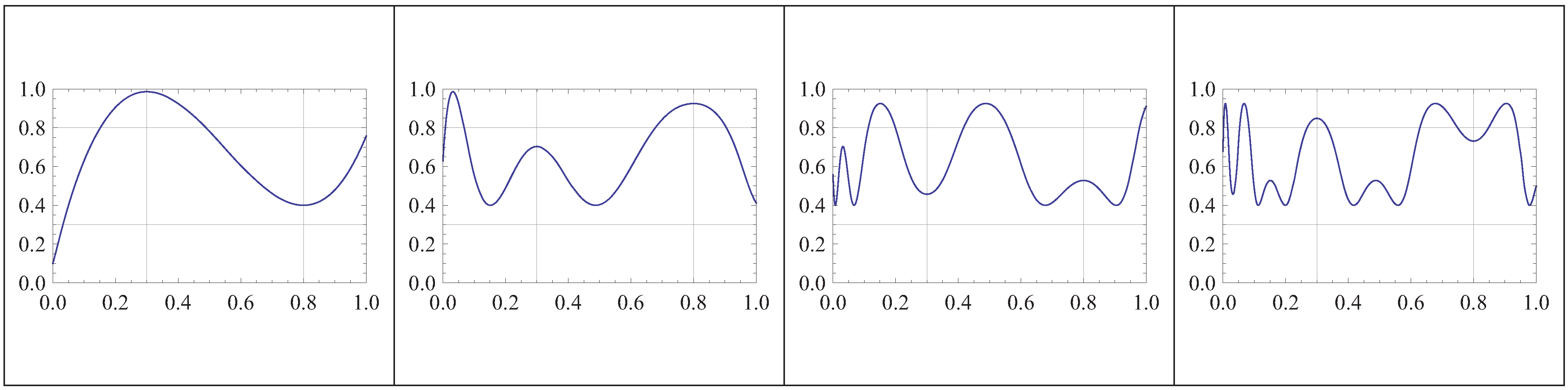
Figure 3 (left) shows the graphs of the full range map , together with and . The convergence rate of to for these three maps when n increases is shown in Figure 3 (right). The precision obtained for in this range of parameters and , is the following:
For , the estimation of has four exact decimal digits.
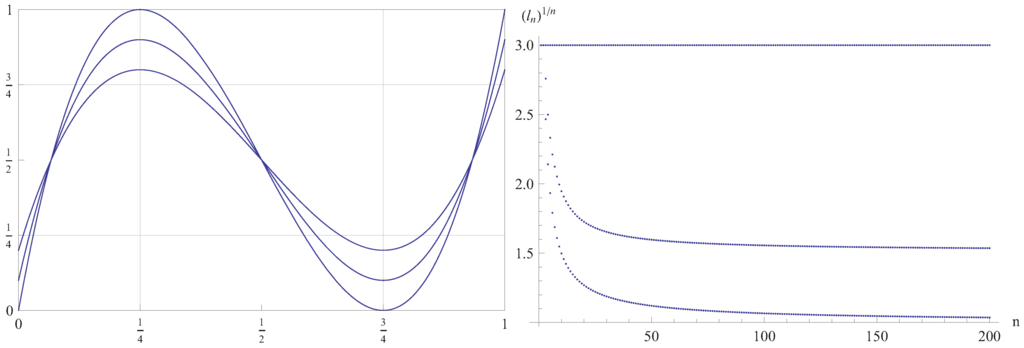
Figure 3.
Left, graphs of the maps . Right, the corresponding convergence plots of to as a function of n (top to bottom).
Figure 3.
Left, graphs of the maps . Right, the corresponding convergence plots of to as a function of n (top to bottom).
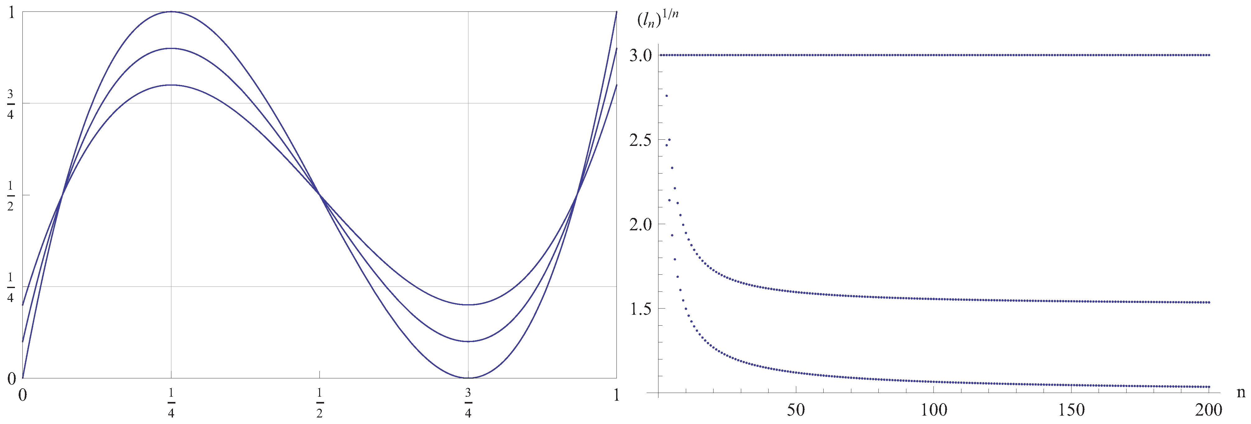
A typical benchmark for estimators of the topological entropy consists in determining the entropy as a function of the control parameter(s). Since depends on two control parameters, we have calculated that dependence both on one parameter (while keeping fixed the other one), and on the two of them. Figure 4 is a plot of vs. . As gets smaller, the number of iterations needed to get the entropy with a given precision grows higher. In Figure 4, the mesh constant used was , and the precision .
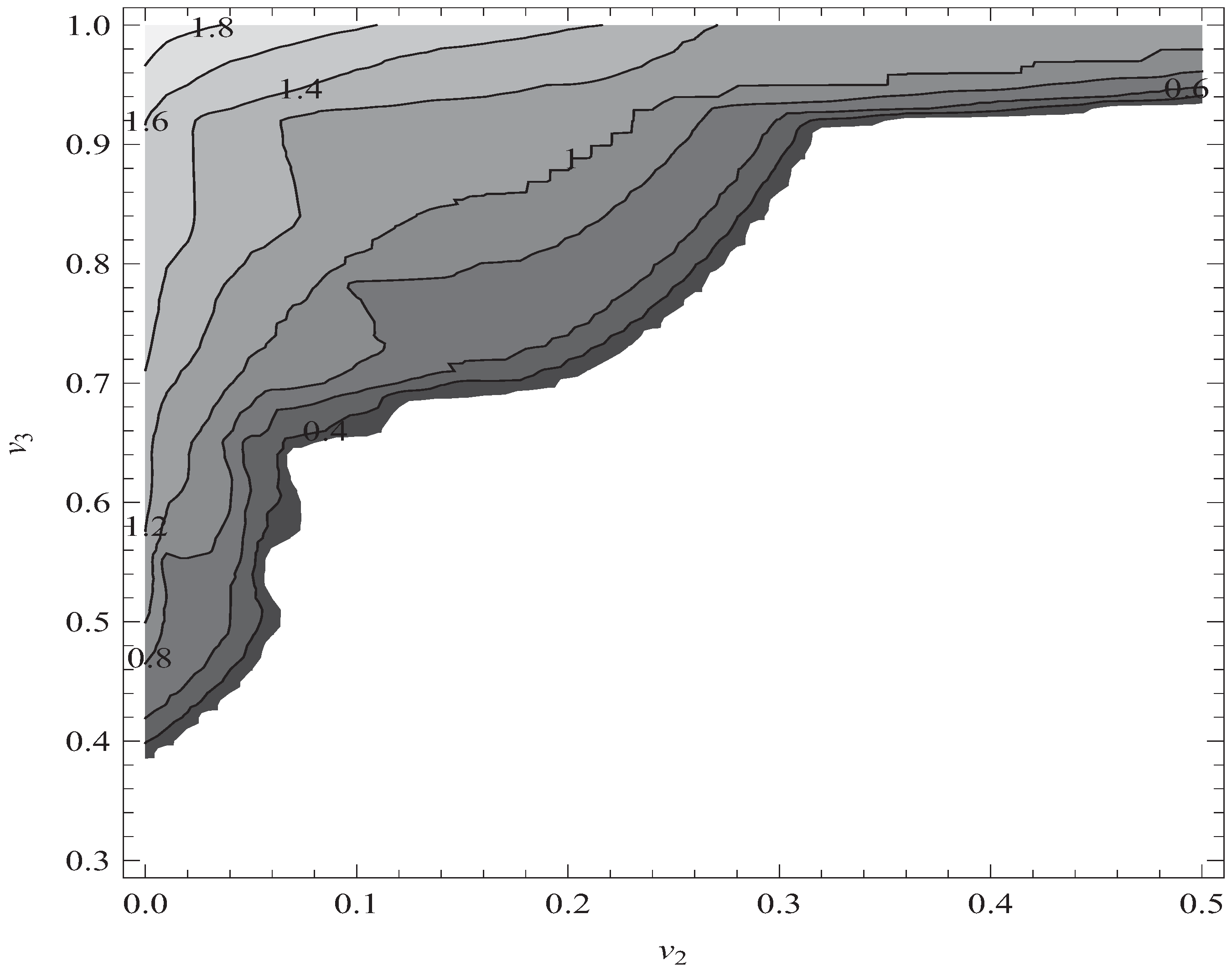
Figure 5 is the same kind of plot, this time for as a function of both control parameters, with , and . This figure depicts also some level sets, just to illustrate the monotonicity of the topological entropy in the parametric space. This property, first conjectured by Milnor and Thurston [17], was later proved for quadratic maps in [18,19]. Only recently did H. Bruin and S. van Strien succeed in proving it also for multimodal maps [20]. The computation parameters were set as follows: .
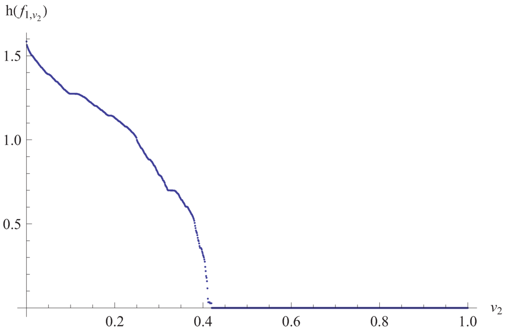
Figure 4.
Plot of vs. , .
Figure 4.
Plot of vs. , .


Figure 5.
Level sets of the plot of vs. , .
Figure 5.
Level sets of the plot of vs. , .
8.2. Simulations with 3-Modal Maps
Consider next the 3-modal maps defined by the quartic polynomials
where . The derivative is
where , and
This family verifies , , , and
Thus, has two fixed critical points ( and ), while the critical point depends on the control parameters , . And again, , coincide with the critical values at and , respectively. The restriction postulated above relates to being a local minimum and a local maximum. Moreover, the left endpoint, , is a fixed point.
In particular, the choice and produces a full range quartic, Figure 6, with equation
Figure 7 (left) shows the dependence of on the control parameter , while Figure 7 (right) does the same for with . As in the previous computation with a uniparametric cubic, , and . Finally, Figure 8 depicts some level sets of with and . Here .
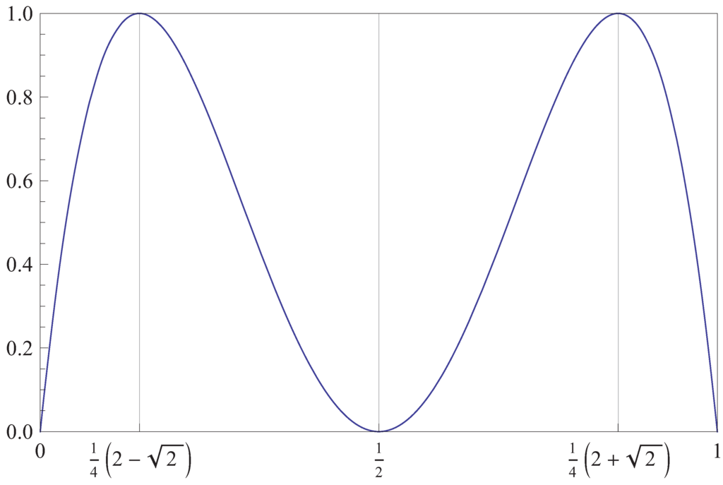
Figure 6.
The full range quartic .
Figure 6.
The full range quartic .
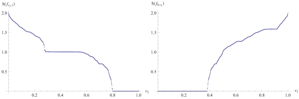
Figure 7.
Left, plot of vs. , . Right, plot of vs. , .
Figure 7.
Left, plot of vs. , . Right, plot of vs. , .

Figure 8.
Level sets of the plot of vs. , .
Figure 8.
Level sets of the plot of vs. , .
9. Conclusions
We have given an algorithm to efficiently calculate the lap number (hence, the topological entropy) for the iterates of a twice differentiable l-modal map f. The algorithm is based on symbolic sequences , , —the min-max sequences of f—that contains qualitative information about the structure of maxima and minima of the map iterates and the orbits of the endpoints. Theorem 6.3 shows that is determined by the initial segments , hence by the itineraries of the critical and boundary points up to order . This approach builds on previous results for unimodal, boundary-anchored maps obtained in [13] and [15] (Corollary 6.4) and [16]. To test if the topological entropy is positive, we test if the kneading sequences are similar or differ from the kneading sequences associated with the Feigenbaum period doubling cascade ([16], Section 5). If the kneading sequences are similar, than the map has zero topological entropy. Finally, we would like to add that the counting techniques developed here can be extended to maps with jump discontinuities and to piecewise continuous and monotonous maps. However in this case, the kneading sequence calculus must be substantially changed.
Acknowledgements
We thank our referees for their kind and valuable comments. J.M.A. is indebted to Lluís Alsedà, Henk Bruin and Jed Keesling for stimulating discussions on the topic of this paper. J.M.A. and A.G. were supported by the Spanish Ministry of Science and Innovation, grant MTM2009-11820.
References
- Adler, R.; Konheim, A.; McAndrew, M. Topological entropy. Trans. Amer. Mat. Soc. 1965, 114, 309–319. [Google Scholar] [CrossRef]
- de Melo, W.; Strien, S. van. One-Dimensional Dynamics; Springer: New York, NY, USA, 1993. [Google Scholar]
- Alsedà, L.; Llibre, J.; Misiurewicz, M. Combinatorial Dynamics and Entropy in Dimension One; World Scientific: Singapore, 2000. [Google Scholar]
- Misiurewicz, M.; Szlenk, W. Entropy of piecewise monotone mappings. Studia Math. 1980, 67, 45–63. [Google Scholar]
- Block, L.; Keesling, J.; Li, S.; Peterson, K. An improved algorithm for computing topological entropy. J. Stat. Phys. 1989, 55, 929–939. [Google Scholar] [CrossRef]
- Block, L.; Keesling, J. Computing the topological entropy of maps pf the interval with three monotone pieces. J. Stat. Phys. 1991, 66, 755–774. [Google Scholar] [CrossRef]
- Collet, P.; Crutchfield, J.P.; Eckmann, J.P. Computing the topological entropy of maps. Comm. Math. Phys. 1983, 88, 257–262. [Google Scholar] [CrossRef]
- Góra, P.; Boyarsky, A. Computing the topological entropy of general one-dimensional maps. Trans. Amer. Math. Soc. 1991, 323, 39–49. [Google Scholar] [CrossRef]
- Balmforth, N.J.; Spiegel, E.A.; Tresser, C. Topological entropy of one-dimensional maps: Approximations and bounds. Phys. Rev. Lett. 1994, 72, 80–83. [Google Scholar] [CrossRef] [PubMed]
- Froyland, G.; Murray, R.; Terhesiu, D. Efficient computation of topological entropy, pressure, conformal measures, and equilibrium states in one dimension. Phys. Rev. E 2007, 76, 036702. [Google Scholar] [CrossRef] [PubMed]
- Baldwin, S.L.; Slaminka, E.E. Calculating topological entropy. J. Stat. Phys. 1997, 89, 1017–1033. [Google Scholar] [CrossRef]
- Steinberger, T. Computing the topological entropy for piecewise monotonic maps on the interval. J. Stat. Phys. 1999, 95, 287–303. [Google Scholar] [CrossRef]
- Dias de Deus, J.; Dilão, R.; Taborda Duarte, J. Topological entropy and approaches to chaos in dynamics of the interval. Phys. Lett. A 1982, 90, 1–4. [Google Scholar] [CrossRef]
- Dias de Deus, J.; Dilão, R.; Taborda Duarte, J. Topological entropy, characteristic exponents and scaling behaviour in dynamics of the interval. Phys. Lett. A 1982, 93, 1–3. [Google Scholar] [CrossRef]
- Dilão, R. Maps of the interval, symbolic dynamics, topological entropy and periodic behavior (in Portuguese). Ph.D. Thesis, Instituto Superior Técnico, Lisbon, Portugal, 1985. [Google Scholar]
- Dilão, R.; Amigó, J.M. Computing the topological entropy of unimodal maps. Int. J. Bifurcat. Chaos Appl. Sci. Eng. 2012, in press. [Google Scholar]
- Milnor, J.; Thurston, W. On iterated maps of the interval. In Dynamical Systems. Lectures Notes in Mathematics; Alexander, J.C., Ed.; Springer: Berlin, Germany, 1988; pp. 465–563. [Google Scholar]
- Douady, A. Topological entropy of unimodal maps: Monotonicity for quadratic polynomials. In Real and Complex Dynamical Systems; Branner, B., Hjorth, P., Eds.; Kluwer: Dordrecht, The Netherlands, 1995; pp. 65–87. [Google Scholar]
- Tsujii, M. A simple proof for monotonicity of entropy in the quadratic family. Erg. Dyn. Sys. 2000, 20, 925–933. [Google Scholar] [CrossRef]
- Bruin, H.; van Strien, S. Monotonicity of entropy for real multimodal maps. arXiv, 2009; arXiv:0905.3377v1. [Google Scholar]
© 2012 by the authors. Licensee MDPI, Basel, Switzerland. This article is an open access article distributed under the terms and conditions of the Creative Commons Attribution license ( http://creativecommons.org/licenses/by/3.0/).