Abstract
Because of the importance of damage detection in manufacturing systems and other areas, many fault detection methods have been developed that are based on a vibration signal. Little work, however, has been reported in the literature on using a recurrence plot method to analyze the vibration signal for damage detection. In this paper, we develop a recurrence plot based fault detection method by integrating the statistical process control technique. The recurrence plots of the vibration signals are derived by using the recurrence plot (RP) method. Five types of features are extracted from the recurrence plots to quantify the vibration signals’ characteristic. Then, the T2 control chart, a multivariate statistical process control technique, is used to monitor these features. The T2 control chart technique, however, has the assumption that all the data should follow a normal distribution. The RP based T2 bootstrap control chart is proposed to estimate the control chart parameters. The performance of the proposed RP based T2 bootstrap control chart is evaluated by a simulation study and compared with other univariate bootstrap control charts based on recurrence plot features. A real case study of rolling element bearing fault detection demonstrates that the proposed fault detection method achieves a very good performance.
1. Introduction
Damage detection is very important in many areas, including aerospace, civil and mechanical engineering systems. Due to the potential economic and life-safety implications, early damage detection has motivated a significant amount of research. The vibration signal is usually collected and used for damage detection. Many vibration based damage detection techniques have been developed and are widely used for monitoring and diagnosis in the areas of condition-based maintenance, structural health monitoring and so forth [1–3]. For example, many signal processing methods have been used to investigate the vibration signals, and features are derived to represent the signal characteristics, such as the frequency domain method, wavelet based analysis and time series based analysis [4–6]. Numerous classification methods or decision making methods have been conducted to obtain detections result based on these features, such as neural network based methods, the support vector machine and the decision tree method [7–9]. A brief review of damage detection based on vibration signals can be found in Carden [10]. However, there is a challenge to analyze these vibration signals in complex system since these vibration signals usually contain complex, nonstationary, noisy and nonlinear characteristics, whose behaviors may range from quasi-periodic to completely irregular [11].
In order to address this challenge, the recurrence plot (RP) method is introduced to develop a new vibration based damage detection method. The RP method, first proposed by Eckmann [12], is considered to be an effective tool for analyzing the nonlinear and nonstationary waveform signal in a dynamic system. This method is a signal process method that can construct a two-dimensional matrix from a one-dimensional waveform signal. One advantage of using the RP method to analyze the vibration signal is that it does not make any assumptions on the data distribution and data size [13]. The RP method can characterize the autocorrelations of the vibration signal over the time-scale. Several features can be extracted by the recurrence quantification analysis (RQA) to describe the characteristic of the signal.
The RP method has been widely used in the area of the medicine, geography, chemistry and other areas. Chen and Yang developed a multi-scale RP method and have employed that method to analyze electrocardiogram signals [14]. Masugi conducted the RP method to do non-stationary transition patterns analysis in IP-network traffic [15]. Du and Song used the RP method to analyze the surface discharge of gamma-ray irradiated polymeric materials [16]. Litak et al. [17] detected the damages of the rotating shaft by using RQA to extract the recurrence feature of the time series data. However, only a few papers are reported in the literature about using the RP method to analyze the vibration signal for damage detection. Nichols et al. used RQA to detect damage-induced changes to the structural dynamics when analyzing the time series signals, but they didn’t develop a monitoring scheme based on the RP method [18]. Some researchers have combined the univariate statistical process control technique with the RP method to develop process monitoring schemes. For example, Tykierko developed a RP based exponentially weighted moving average (EWMA) control chart to detect changes in the complex system by integrating the control chart techniques with the RP method [19]. However, in his method, only one feature is used to characterize the system.
In order to fully use the information extracted by the RP method, we propose a vibration-based fault detection method by integrating the recurrence plot (RP) method and Hotelling’s T2 control chart technique in this paper. The Hotelling’s T2 control chart, which is introduced by Hotelling, is a multivariate statistical process control technique that can monitor vibration signals by using all the features extracted from the recurrence plot [20]. The T2 control chart requires that the features should follow multivariate normal distribution. However, we do not have the distribution information of these features extracted by the RQA method and we cannot conclude that these features follow multivariate normal distribution.
To address this problem, the nonparametric bootstrap method is introduced to build the T2 bootstrap control chart. The bootstrap, a kind of resampling method, can be used to estimate the sampling distribution of a statistic while assuming only that the observations are independent and identically distributed. Bajgier proposed a bootstrap control chart to monitor the mean of a process [21]. In this paper, we extend the Bajgier’s bootstrap control chart to the T2 control chart case to develop a T2 bootstrap control chart. However, Seppala pointed out that there is an obvious limitation in that Bajgier’s bootstrap control chart implicitly assumes that the process is stable and in-control when the control limits are computed [22]. If this assumption is violated, the control limits computed will be too wide. For this reason, a pre-process method is developed to remove the outliers based on the RP method before conducting the bootstrap method.
In this paper, the concepts of the RP method and the RQA are introduced first. Second, we propose a damage detection scheme based on RP method and T2 control chart technique to monitor process conditions. Then, we compare our proposed damage detection scheme with other RP based univariate control charts method to show the performance of our proposed method. At last, a real case of rolling element bearing damage detection is studied to demonstrate our proposed method and conclusions are given.
2. Review of the RP Method
In this section, we will briefly introduce the RP method and the RQA. An example is given to show the RP method. Five features of RP method obtained by RQA are interpreted.
2.1. Introduction of RP Method
Denote X = [X1, X2, …, XN]T as a series of vibration signals with N points each. Then a series of d -dimensional vectors
can be constructed from the one-dimensional signal {Xi} by using Equation (1).
where d and τ are called embedding dimension and time delay, and N′ = N – (d − 1) · τ. The vectors
represent the signal trajectories in phase space. If we define a threshold ξ, then a two-dimensional matrix can be obtained by comparing the distance between the vectors in
with ξ as shown in Equation (2).
where ‖ · ‖ is a norm function and Θ (·) is the Heaviside function. R is called recurrence matrix with N′ columns and N′ rows. R(i, j) represents the element with row i and column j. If the distance between
and
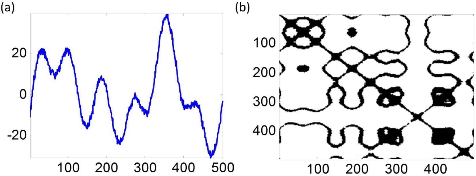
is less than the threshold ξ, Ri,j = 1, otherwise Ri,j = 0. If we plot the element “1” as black dot and plot the element ‘0’ as white dot, then we can conclude that the R can be visualized as a binary image, which is named as RP graph is this paper. Figure 1 is an example to show the RP method. Figure 1a shows a simulated signal, and Figure 1b is its RP graph.

Figure 1.
An example of recurrence plot method: (a) a simulated signal and (b) the corresponding recurrence plot (RP) plot.
There are three important parameters in the RP method: the embedding dimension d, the time delay τ and the threshold ξ. Many researchers have already developed rules to determine them. In this paper, we used the false nearest neighbors (FNN) algorithm and the mutual information method to determine the embedding dimension d and the time delay τ [23,24]. According to Thiel, the threshold ξ should be five times larger than the standard variation of the given signal [25].
2.2. Recurrence Quantification Analysis
According to the introduction above, we can see that the RP graph consist of the single points, the diagonal lines, the vertical lines, and the horizontal lines. Based on Equation (2), we can conclude that the RP graph is a symmetrical matrix. Therefore the horizontal lines have the same meaning as the vertical lines. These various structures reflect the autocorrelation of the signal in the time scale [13]. Based on these structures of the RP graph, Zbilut developed a series of features including recurrence rate (RR), determinism (DET) and entropy (ENT) based on the single points and the diagonal lines structures [26]. Marwan developed laminarity (LAM) and trapping time (TT) based on the vertical lines [27]. The detailed introductions of these features are provided below. In the following equations, P(l) is the histogram of the diagonal lines with the length l, lmin is the minimal length of the diagonal lines, P(v) is the histogram of the vertical lines with the lengths v, and vmin is the minimal length of the vertical lines.
- (1)
- Recurrence Rate (RR)RR is a feature to measure the density of the black dots in the RP graph. A larger RR value means more black dots in the RP graph. The RR can characterize the signal’s stationarity, periodicity and complexity.
- (2)
- Determinism (DET)DET represents the proportion of the black dots forming the diagonal lines which are longer than lmin. According to Marwan [13], the diagonal line refers to the recurrences of the original signal in the corresponding signal segments. The DET measures the occurrence of diagonal lines with different lengths in the RP plot.
- (3)
- Entropy (ENT)ENT represents the Shannon information entropy of the selected diagonal lines whose lengths are longer than lmin, and it reflects the complexity of the RP in respect of the diagonal lines.
- (4)
- Laminarity (LAM)LAM measures the proportion of the black dots forming the vertical lines which are longer than vmin. The vertical lines have the same interpretation as the horizontal lines which are caused by the slow changes from a certain signal value in the original signal. Hence, LAM is a measure of the occurrence of vertical lines in the RP plot.
- (5)
- Trapping time (TT)TT calculates the average length of the vertical lines which are longer than vmin, and it represents the average length of the vertical lines in RP plots.
Then, we can obtain a vector that Y = [RR, DET, ENT, LAM, TT] as the feature to represent the signal. In the following section, the T2 control chart is constructed based on this vector Y to monitor the signal.
3. Methodology Development
This section presents the proposed damage detection scheme that integrates the RP methodology and the T2 control chart technique. First, the RP method is conducted on the collected signals and five features are extracted. The T2 control chart is then introduced and used to monitor the five features. After that, the nonparametric bootstrap method is introduced to estimate the control limit of the T2 control chart.
3.1. T2 Control Chart Based on the RP Method
The T2 control chart, which is also called Hotelling T2 control chart, is widely used in multivariate statistical process control [20]. We assume we have p variables x1, x2, …, xp and then we obtain a group of samples X = [X1, X2, …, Xp]. Assuming the samples follow a multivariate normal distribution, then the sample mean vector is
and the sample covariance matrix is
, where N is the sample number of each variable. Thus, the T2 statistic is
where n is the sample size.
Assume u = {u1, u2, … uN} is a group of vibration signals. Then the RP graph {R1, R2, RN} can be derived and RR, DET, ENT, LAM, TT can be estimated by RQA. Defining Y = [RR, DET, ENT, LAM, TT], a T2 control chart based on the RP method can be constructed based on the Y. The T2 statistic based on RP method can be obtained as
The control limit of the RP-based T2 control chart needs to be estimated here. Usually, there are two distinct phases, which are Phase I and Phase II when we use the control chart techniques. In Phase I, the main goals are estimating the control chart parameters and removing the outliers. We do not have any prior information on deriving appropriate control limits. Therefore, after a group of process data is collected, some pre-process algorithms or de-noising methods are used to remove the outliers. Then estimate the distribution of the data and the control chart parameters to build a control chart. After that, test the data by using the control chart. Then remove the out-of-control data and rebuild the control chart until all data is in-control. In Phase II, the major goal is to detect changes in the newly observed data. The estimated in-control data distribution from the Phase I dataset is used. The performance of a Phase II procedure is often measured from the view point of the Average Run Length (ARL), which is defined as the average number of samples taken before the chart triggers a signal [28]. Usually, the in-control ARL is controlled at a specific level with a defined false alarm rate α. For example, people often set the in-control ARL of the
control chart to ARL=370 with the false alarm rate α = 0.027 when the in-control data follows normal distribution. The out-of-control ARL is used to measure the performance of the control chart so that the control chart performs better if the out-of-control ARL is smaller when detecting a given change. Please refer to Montgomery to see a detailed introduction about Phase I and Phase II analysis [29]. Traditionally, if we assume that the observed data follows multivariate normal distribution, then the Phase I control limit of the T2 control chart is UCL = (m − 1)(n − 1)p/(m(n − 1) + 1 − p) · Fα(p, m(n − 1) + 1 − p) and the Phase II control limit is UCL = (m + 1)(n − 1)p/(m(n − 1) + 1 − p) · Fα(p, m(n − 1) + 1 − p), where m is the samples number used for training the control limit in Phase I. The parameter α is the false alarm rate, which means the probability of T2 > UCL is α when the data is in-control. However, we cannot obtain the distribution information of the defined variable Y. Therefore the nonparametric bootstrap method is used to estimate the control limit.
3.2. Bootstrap Method
As mentioned above, the RP-based T2 statistic and control limits are estimated with the assumption that the samples follow multivariate normal distribution. However, we cannot ensure that the features vector Y = [RR, DET, ENT, LAM, TT] is multivariate with a normal distribution. To address this problem, the bootstrap method is used to estimate the T2 statistic and the control limit of the T2 control chart. First, we apply the concept of the nonparametric bootstrap to estimate the sample mean and the sample covariance of the vector Y. Then the T2 statistic is obtained and the control limit of T2 control chart is estimated.
Suppose we have a random variable X = (x1, x2, … xn) and the underlying cumulative distribution function of X is F(x). Assigning a probability of 1/n to each value in X, the empirical distribution function can be written as:
The
converges to F(x) as n → ∞. The central limit theorem states that
has an asymptotically normal distribution when the sample number n is large enough. Thus, we can assume that the random variable X follows normal distribution if n → ∞.
Based on the introduction of the empirical distribution function, we can assume that the vector Y = (Y1, Y2, …, Yn) follows a multivariate normal distribution if we can obtain enough sample numbers. Then the T2 statistic can be obtained and the control limit of the T2 bootstrap control chart can be estimated based on Bajgier’s method.
Thus, the procedures of deriving the control limit of the proposed T2 bootstrap control chart are provided as follows.
- Assume we obtain a group of in-control process signals {x1, x2, … xn}. Conduct the RP method to analyze the signals to obtain the recurrence plots {R1, R2, … Rn}.
- Conduct the RQA to extract features of the {R1, R2, … Rn} in order to obtain the vectors {Y1, Y2, … Yn}
- Obtain the T2 statistic according to to get a group of T2 statistic values , where and S are the sample mean and sample covariance of the vectors {Y1, Y2, …, Yn}, respectively.
- Draw a random sample of size nc, such as nc = 100,000, with replacement, from the samples , then get the sample , which is a bootstrap sample.
- Sort the bootstrap T2 statistic in ascending order to derive . Find the value that , where i = 1, 2, …, nc. Thus, the T2 bootstrap control chart’s control limit is .
3.3. Damage Detection Scheme
In this subsection, a damage detection scheme is proposed to analyze the vibration based signals by using the RP-based T2 control chart. Following the notations introduced earlier, the procedures of the proposed damage detection scheme are stated as follows. Figure 2 shows the framework of the proposed monitoring scheme.
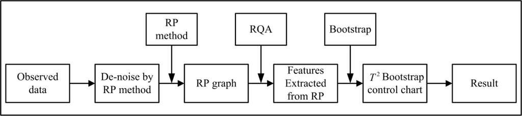
Figure 2.
The proposed damage detection scheme.
- Collect a group of system vibration signals {u1, u2, … un} under normal conditions.
- Conduct the RP method to analyze the vibration signals and extract the five features RR, DET, ENT, LAM, TT by RQA and obtain the feature vector Yi = [RR, DET, ENT, LAM, TT], i = 1,2, ⋯, n.
- Estimate the sample mean and sample covariance S of the vectors Yi, and then obtain the T2 statistic according to the equation .
- Estimate the control limit UCL of the proposed T2 bootstrap control chart according to the procedures introduced in section bootstrap method.
- When a new system vibration signal is collected, use the RP method and RQA method to obtain the feature vector Ynew = [RR, DET, ENT, LAM, TT].
- Obtain the T2 statistic according to the equation . Monitor this T2 statistic using the proposed RP-based T2 bootstrap control chart. If , we can conclude that the signal is out-of-control. It means a process fault occurred in the system. If we can conclude that the signal is in-control and the system is in a normal condition.
4. Performance Evaluation
In this subsection, we evaluate the performance of our proposed damage detection scheme and then compare the proposed RP-based T2 bootstrap control chart with other RP-based univariate control charts which are the RQA-based univariate control charts in terms of the average run length (ARL). Here, the RQA-based univariate control charts are constructed based on the five RP features introduced in Section RQA introduction. These five features are RR, DET, ENT, LAM and TT. For simplicity, the RQA-based control charts are named the RR-based control chart, the DET-based control chart, the ENT-based control chart, the LAM-based control chart and the TT-based control chart. Without loss of generality, we will compare the monitoring performance of the proposed RP-based T2 bootstrap control chart and the RQA-based control charts in order to analyze the simulated signals. The out-of-control ARLs are compared when detecting the mean shift case and the frequency change case. The steps for obtaining the out-of-control ARLs of the RP-based T2 bootstrap control chart and the RQA-based control charts are stated as follows.
- Step 1.
- According to the procedures introduced in section T2 control chart based on the RP method, obtain the control limits of the RP-based T2 bootstrap control chart and the RQA-based control charts of the simulated in-control signals.
- Step 2.
- Simulate groups of out-of-control signals with mean shift or frequency change. Obtain the five features (RR, DET, ENT, LAM and TT) by RQA and the T2 statistic .
- Step 3.
- Estimate the run length (RL) of the RP-based T2 bootstrap control chart and the RQA-based control charts with the false alarm rate α = 0.05.
- Step 4.
- Repeat the above steps np = 5000 times to obtain the out-of control ARLs of the RP-based T2 bootstrap control chart and the RQA-based control charts for the mean shift case or the frequency change case.
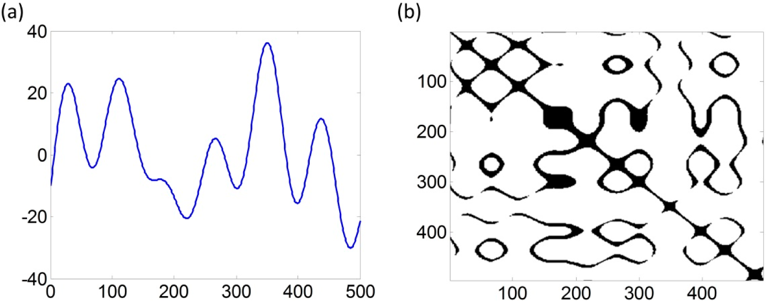
Denote f0 = D + ξ as the in-control signal, f′ = f0 + F as the out-of control signal, D as the main process effect under in-control condition, F as the signal change component and ξ as the process noise. Without loss of generality, we assume the process noise ξ follows a normal distribution and can be represented as ξ ~ σNoise · N(0,1). Denote AF as the amplitude of F, and then define δF = AF/σNoise to measure the magnitude of the signal change component. Figures 3–5 are examples to show the original signals and their RP graphs of the in-control case, the mean shift case with δF = 1.5 and the frequency change case with δF = 1.5. We can see that there are some differences among the three in-control and out-of-control RP graphs although the original signals of the in-control and out-of-control cases are seen as the same. We will conduct our proposed damage detection scheme on the simulated signals to show that our proposed method is effective for detecting small or large signal change.
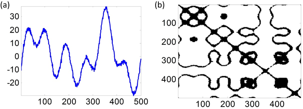
Figure 3.
An example of the simulated in-control signals and its RP graph: (a) simulated in-control signal, (b) the RP graph of the in-control signal.
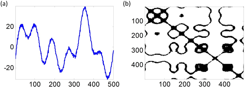
Figure 4.
An example of the simulated signals and its RP graph of the mean shift case with δF = 1.5: (a) simulated out-of-control signal, (b) the RP graph of the out-of-control signal.
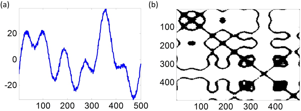
Figure 5.
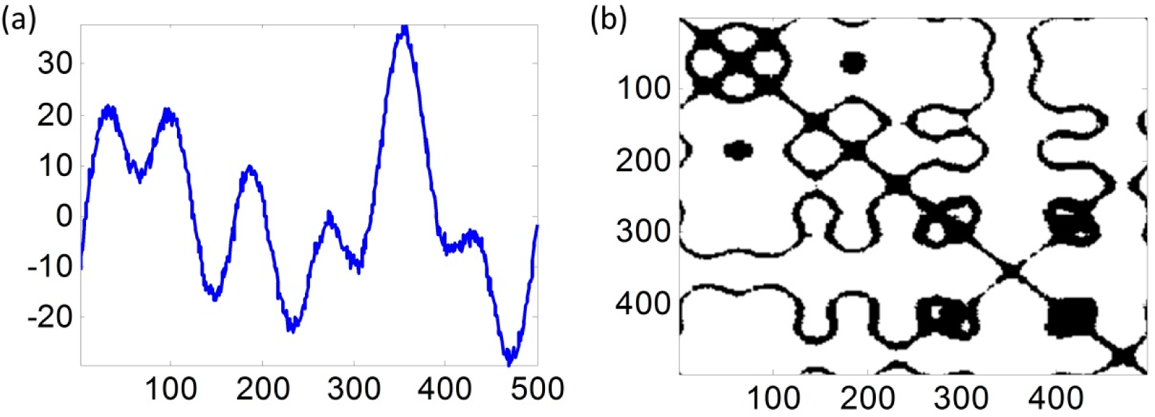
An example of the simulated signals and its RP graph of the frequency change case with δF=1.5: (a) simulated out-of-control signal, (b) the RP graph of the out-of-control signal.
In detecting the mean shift case, F represents the component of the signal mean shift. The frequency information in F is same as that in the component f0 · δF measures the magnitude of the signal shift component. Table 1 shows the out-of control ARLs in detecting the mean shift case.

Table 1.
Average Run Length (ARL) comparison for mean shift case.
In detecting the frequency change case, F represents the component of frequency change. The frequency information in F is different with the one in the component f0 · δF measures the magnitude of the frequency change component. Table 2 shows the out-of-control ARLs in detecting the frequency change case.
Table 2.
ARL comparison for frequency change case.
The out-of-control ARL is the average number of samples taken before the out-of-control condition is detected by the designed control chart. The small ARL value means the designed control chart can detect the out-of-control condition quickly. In Tables 1 and 2, first, we can see that all the out-of-control ARLs of the proposed RP-based T2 bootstrap control chart are small and will be even smaller when δF is increasing in both the mean shift case and frequency change case. Second, the out-of-control ARLs of the proposed RP-based T2 bootstrap control chart are always the smallest when compared with the other RQA based control charts. Therefore, we can conclude that: (1) the proposed damage detection scheme can detect both small and large signal changes effectively and efficiently; (2) the proposed RP-based T2 bootstrap control chart uniformly performs better than any other RQA based control charts.
5. Case Study
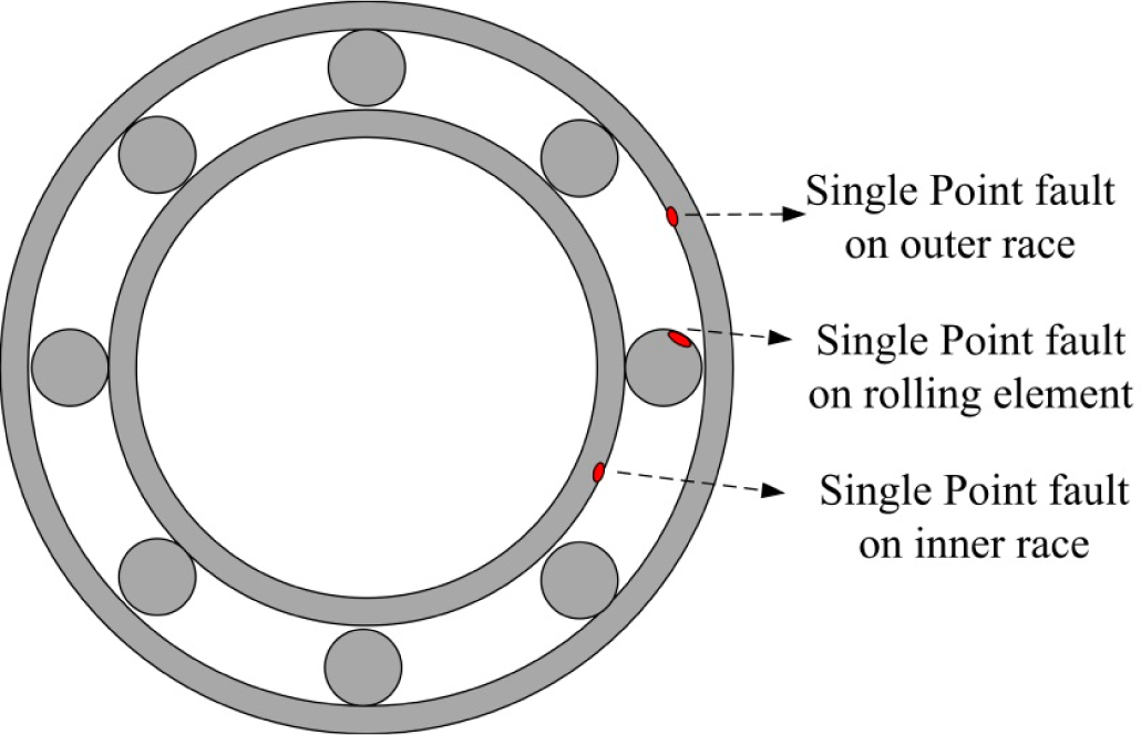
In this section, we use a real example of a rolling element bearing fault detection to demonstrate our proposed method. The rolling element bearings, widely used in various areas of industry, are the most critical components in rotating electrical machinery due to the fact that the large majority of problems arise from faulty bearings. Rolling element bearings generally consist of two rings (which are called the outer race and the inner race) with a set of rolling elements rotating in their tracks. Faults on the bearings such as wear, cracks, and pits can cause malfunctions and catastrophic failures. In this case, we investigate single point faults that occur on the inner race, outer race, and rolling element. Figure 6 shows an example of the rolling element bearing and the three types of single point faults.

Figure 6.
The rolling element bearing.
5.1. Data Introduction
In this case, we use the seeded fault test data provided by the Case Western Reserve University Bearing Data Center to demonstrate our proposed fault detection method by integrating the RP method and the RP based T2 bootstrap control chart [30]. The experiment equipment consists of a motor (left), a torque transducer/encoder (center), a dynamometer (right), and control electronics. The test bearings support the motor shaft. Single point faults were introduced into the test bearings with different fault diameters. Vibration data was collected using accelerometers, which were attached to the housing by use of magnetic bases. Data was collected for normal bearings, a single point fault occurring on the inner race, on the outer race and on the rolling element. Please refer Bearing Data Center website26 for more instructions about the data set.
In order to demonstrate the successful performance of our proposed method, we choose the case in which the bearing fault signal is collected with a 12 k load and where the fault diameter is seven mils (a thousandth of an inch), which is the smallest one. We extracted 300 samples from a normal bearing vibration data set, which is named the “NB” group. Then, we extracted 90 samples in each group of the bearing faults that occurred on the inner race, the outer race and the rolling element. These are named “FIR”, “FOR” and “FRE” respectively.
5.2. Feature Extraction
Following the procedures introduced in section bootstrap method, the proposed fault detection method is used to analyze the bearing vibration signals. Figure 7a,b show normal bearing signal in the group “NB”and fault signal in “FRE”respectively as an example. Their RP graphs are showed in Figure 7c,d respectively. We can see there is an obvious difference between the normal signal and the fault signal.
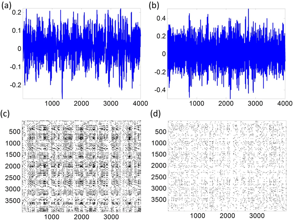
Figure 7.
The RP graphs of normal and fault bearing vibration signals: (a) normal bearing vibration signal, (b) fault bearing vibration signal in “FRE”group, (c) RP graph of normal bearing vibration signal, (d) RP graph of fault bearing vibration signal in “FRE”group.
5.3. Training Control Limit
The control limit of the RP based T2 bootstrap control chart can be obtained based on the procedures mentioned before. Here we use 250 samples in group “NB”as training group to train the control chart. 50 samples are used as testing group to test the RP based T2 bootstrap control chart. Here, we set the false alarm rate α = 0.05. Figure 8 shows the testing result of the RP based T2 bootstrap control chart. The horizontal axis is the sample index and the vertical axis is the derived T2 statistic value of the testing group data. The straight solid line is the control limit of the RP based T2 bootstrap control chart estimated from the training group data with defined false alarm rate α = 0.01 in this case. Each point in the Figure 8 represents the T2 statistic value of each sample in the testing group data. According to the control chart theory, if all statistic values are below the control limit, it means all the samples are in-control. From Figure 8, we can see that all the points are below the solid line which is the control limit of the RP based T2 bootstrap control chart. Therefore, we can conclude that our proposed RP based T2 bootstrap control chart works well to monitor the bearing signals in normal condition. Hence, this RP based T2 bootstrap control chart can be used to detect the conditions of the rolling element bearing.
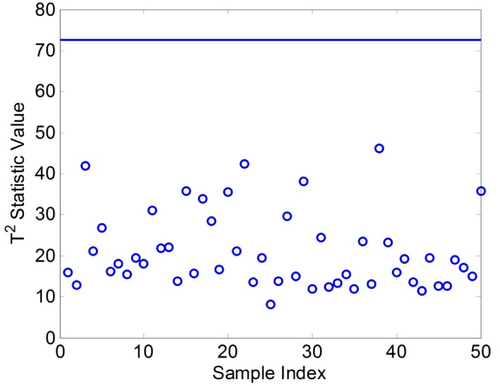
Figure 8.
The testing result of the T2 bootstrap control chart.
5.4. Results
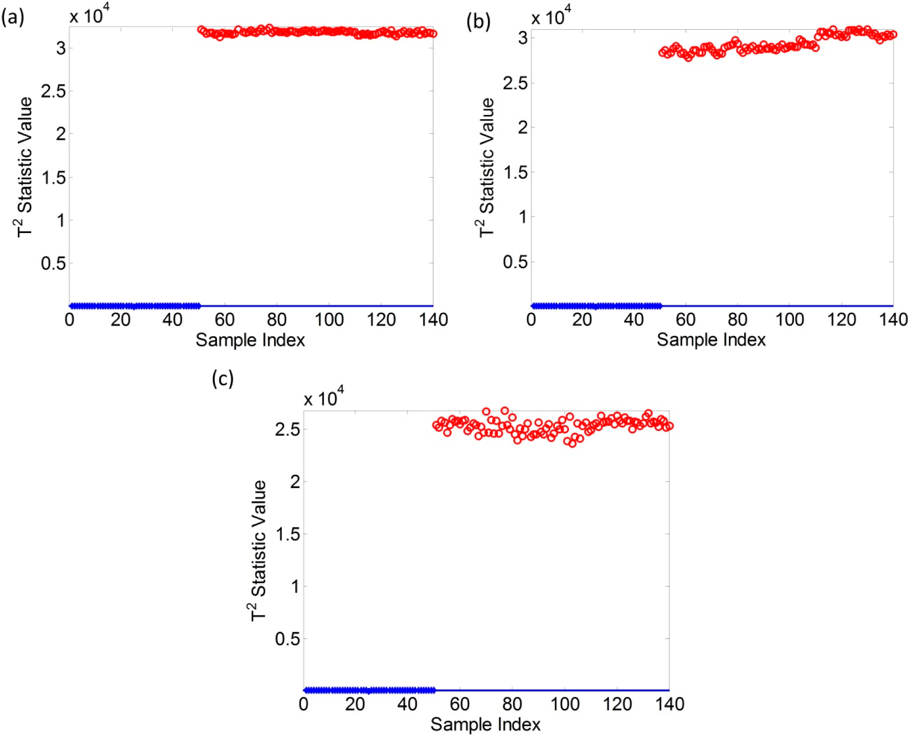
All samples in “FIR”, “FOR” and “FRE” groups are analyzed by the recurrence plot method and the T2 statistics of all samples are calculated. These T2 statistics are tested by the constructed RP based T2 bootstrap control chart as shown in Figure 8. Thus, the conditions of rolling element bearing can be detected by the proposed method. Figure 9a, c show the detection results that the samples are come from the group “FIR”, “FOR” and “FRE”, which means the bearing fault occurred on the inner race, the outer race and the rolling element respectively. In Figure 9, the points marked as red circles represent the fault bearing signals and the points marked as blue stars at the bottom of each figure represent the normal bearing signals, while the blue solid line represents the control limit of the constructed RP based T2 bootstrap control chart. Due to the large difference of the values of the T2 statistics of faulty vibration signals and normal vibration signals, we cannot see blue points and the solid line clearly. Fortunately, all the blue points and the solid line are the same as the blue points and blue line in Figure 8. Therefore, we can consider Figure 8 as enlarged views of the bottom parts in Figure 9. All the red points in Figure 9 are located at the top of the solid line. Therefore, we can conclude that the constructed RP based T2 bootstrap control chart can successfully detect the bearing faults occurred on the inner race, the outer race and the rolling element. Moreover, the values of red points in Figure 9a,b,c are in different intervals, which means the T2 statistic also can be used to diagnose the bearing faults for further research.

Figure 9.
The detection result of fault bearing vibration signals: (a) the T2 control chart of group “FIR”; (b) the T2 control chart of group “FOR”; (c) the T2 control chart of group “FRE”.
According to these figures, we can conclude that our proposed fault detection method by integrating the RP method and the T2 control chart technique performs very well in detecting different types of bearing faulty vibration signals.
6. Conclusions
This paper proposed a damage detection scheme to detect the vibration-based signal change by integrating the RP method and T2 control chart for condition-based maintenance, structural health monitoring, and so forth. The RP method is a nonparametric and nonlinear signal processing method that can characterize the vibration-based signal to be a two dimensional matrix. Five recurrence plot features can be obtained from the two dimensional matrix and can be used to classify vibration signals in normal conditions and in fault conditions. There are several advantages to analyzing the vibration-based signal by using the RP method: (1) it is not necessary to know the information of signal distribution, (2) the method does not require the signal length, (3) the method is a nonparametric method and it is not necessary to estimate the model parameter, (4) the method does not require consideration of the frequency change or the amplitude change in the signal.
In order to monitor the five features, we integrate the statistical process control technique and the bootstrap method to propose a RP based T2 bootstrap control chart. A simulation study has shown that the proposed damage detection scheme can detect signal shift and frequency change quickly and effectively. A real case study of rolling element bearing faults demonstrates that the proposed damage detection scheme can achieve a very good performance in detecting different types of bearing fault.
This paper attempts to introduce the RP method and statistical process control techniques for damage detection. The proposed damage detection scheme also can be used to analyze other waveform signals in addition to the vibration-based signals. Moreover, this scheme can be used in many areas. For different applications, researchers can choose different recurrence plot features to characterize the signal.
Acknowledgments
This article is supported by the National Natural Science Foundation of China (Grant No. 61273205), the Fundamental Research Funds for the Central Universities (Grant No. FRF-SD-12-028A) and the 111 Project (Grant No. B12012).
Author Contributions
In this paper, Cheng Zhou provides the original ideas, completes the calculation and the simulation work, and is responsible for drafting and revising the whole paper; Weidong Zhang contributes to revise the paper and gives some valuable comments on revising the paper. Both authors have read and approved the final manuscript.
Conflicts of Interest
The authors declare no conflict of interest.
References
- Oberst, S.; Lai, J.C.S. Statistical Analysis of Brake Squeal Noise. J. Sound Vib 2011, 330, 2978–2994. [Google Scholar]
- Wernitz, B.A.; Hoffmann, N.P. Recurrence Analysis and Phase Space Reconstruction of Irregular Vibration in Friction Brakes: Signatures of Chaos in Steady Sliding. J. Sound Vib 2012, 331, 3887–3896. [Google Scholar]
- Kuo, Y.C.; Hsieh, C.T.; Yau, H.T.; Li, Y.C. Research and Development of a Chaotic Signal Synchronization Error Dynamics-based Ball Bearing Fault Diagnostor. Entropy 2014, 16, 5358–5376. [Google Scholar]
- Parker, B.E.; Ware, H.A.; Wipe, D.P.; Tompkins, W.R.; Clark, B.R. Fault Diagnostics Using Statistical Change Detection in the Bispectral Domain. Mech. Syst. Signal Process 2000, 14, 561–570. [Google Scholar]
- Hou, Z.; Noori, M.N.; Amand, R.S. Wavelet-based Approach for Structural Damage Detection. J. Eng. Mech 2000, 126, 677–683. [Google Scholar]
- Sohn, H.; Farrar, C.R. Damage Diagnosis Using Time Series Analysis of Vibration Signals. Smart Mater. Struct 2001, 10, 446–451. [Google Scholar]
- Samanta, B.; Al-Balushi, K. Artificial Neural Network Based Fault Diagnostics of Rolling Element Bearings Using Time-domain Features. Mech. Syst. Signal Process 2003, 17, 317–328. [Google Scholar]
- Li, N.; Zhou, R.; Hu, Q.; Liu, X. Mechanical Fault Diagnosis Based on Redundant Second Generation Wavelet Packet Transform, Neighborhood Rough Set and Support Vector Machine. Mech. Syst. Signal Process 2012, 28, 608–621. [Google Scholar]
- Sakthivel, N.; Sugumaran, V.; Babudevasenapati, S. Vibration Based Fault Diagnosis of Monoblock Centrifugal Pump Using Decision Tree. Expert Syst. Appl 2010, 37, 4040–4049. [Google Scholar]
- Carden, E.P.; Fanning, P. Vibration Based Condition Monitoring: A Review. Struct. Health Monit 2004, 3, 355–377. [Google Scholar]
- Hively, L.M.; Protopopescu, V.A. Machine Failure Forewarning via Phase-space Dissimilarity Measures. Chaos 2004, 14, 408–419. [Google Scholar]
- Eckmann, J.P.; Kamphorst, S.O.; Ruelle, D. Recurrence Plots of Dynamical Systems. Europhys. Lett 1987, 4, 973–977. [Google Scholar]
- Marwan, N.; Romano, M.C.; Thiel, M.; Kurths, J. Recurrence Plots for the Analysis of Complex Systems. Phys. Rep 2007, 438, 237–329. [Google Scholar]
- Chen, Y.; Yang, H. Self-organized Neural Network for the Quality Control of 12-lead ECG Signals. Physiol. Meas 2012, 33, 1399–1419. [Google Scholar]
- Masugi, M. Recurrence Plot Based Approach to the Analysis of IP-network Traffic in terms of Assessing Nonstationary Transitions over Time. IEEE Trans. Circuits Syst 2006, 53, 2318–2326. [Google Scholar]
- Du, B.X.; Dong, D.S. Recurrence Plot Analysis of Discharge Currents in Tracking Tests of Gamma-ray Irradiated Polymers. IEEE Trans. Dielectr. Electr. Insul 2008, 15, 974–981. [Google Scholar]
- Litak, G.; Sawicki, J.T.; Kasperek, R. Cracked Rotor Detection by Recurrence Plots. Nondestruct. Test. Eva 2009, 24, 347–351. [Google Scholar]
- Nichols, J.M.; Trickey, S.T.; Seaver, M. Damage Detection Using Multivariate Recurrence Quantification Analysis. Mech. Syst. Signal Process 2006, 20, 421–437. [Google Scholar]
- Tykierko, M. Using Invariants to Change Detection in Dynamical System with Chaos. Physica D 2008, 237, 6–13. [Google Scholar]
- Hotelling, H. Multivariate Quality Control Illustrated by the Testing of Sample Bomb Sights. In Selected Techniques of Statistical Analysis; Eisenhart, .O., Ed.; publisher; Mcgraw-Hill: New York, UK, 1947; Chapter II; pp. 113–184. [Google Scholar]
- Bajgier, S.M. The Use of Bootstrapping to Construct Limits on Control Charts. Proceedings of the Annual Meeting of Decision Science Institute, San Francisco, CA, USA, 22–24 November 1992; pp. 1611–1613.
- Seppala, T.; Moskowitz, H.; Plante, R.; Tang, J. Statistical Process Control via the Subgroup Bootstrap. J. Qual. Technol 1995, 27, 139–153. [Google Scholar]
- Kantz, H.; Schreiber, T. Nonlinear Time Series Analysis; Cambridge University Press: Cambridge, UK, 1997. [Google Scholar]
- Fraser, A.M.; Swinney, H.L. Independent Coordinates for Strange Attractors from Mutual Information. Phys. Rev. A 1986, 33, 1134–1140. [Google Scholar]
- Thiel, M.; Romano, M.C.; Kurths, J.; Meucci, R.; Allaria, E.; Arecchi, F.T. Influence of Observational Noise on the Recurrence Quantification Analysis. Physica D 2002, 171, 138–152. [Google Scholar]
- Zbilut, J.P.; Webber, C.L. Embeddings and Delays as Derived from Quantification of Recurrence Plots. Phys. Lett. A 1992, 171, 199–203. [Google Scholar]
- Marwan, N.; Wessel, N.; Meyerfeldt, U.; Schirdewan, A.; Kurths, J. Recurrence-plot-based Measures of Complexity and their Application to Heart-rate-variability Data. Phys. Rev. E 2002, 66, 026702. [Google Scholar]
- Xiang, L.; Tsung, F. Statistical Monitoring of Multistage Processes Based on Engineering Models. IIE Trans 2008, 40, 957–970. [Google Scholar]
- Montgomery, D.C. Introduction to Statistical Quality Control, 5th ed; Wiley: New York, NY, USA, 2003. [Google Scholar]
- Bearing Data Center: Seeded Fault Test Data; Case Western Reserve University. Available online: http://csegroups.case.edu/bearingdatacenter/home accessed on 5 September 2014.


© 2015 by the authors; licensee MDPI, Basel, Switzerland This article is an open access article distributed under the terms and conditions of the Creative Commons Attribution license (http://creativecommons.org/licenses/by/4.0/).