Learning a Flexible K-Dependence Bayesian Classifier from the Chain Rule of Joint Probability Distribution

Abstract

As one of the most common types of graphical models, the Bayesian classifier has become an extremely popular approach to dealing with uncertainty and complexity. The scoring functions once proposed and widely used for a Bayesian network are not appropriate for a Bayesian classifier, in which class variable C is considered as a distinguished one. In this paper, we aim to clarify the working mechanism of Bayesian classifiers from the perspective of the chain rule of joint probability distribution. By establishing the mapping relationship between conditional probability distribution and mutual information, a new scoring function, Sum_MI, is derived and applied to evaluate the rationality of the Bayesian classifiers. To achieve global optimization and high dependence representation, the proposed learning algorithm, the flexible K-dependence Bayesian (FKDB) classifier, applies greedy search to extract more information from the K-dependence network structure. Meanwhile, during the learning procedure, the optimal attribute order is determined dynamically, rather than rigidly. In the experimental study, functional dependency analysis is used to improve model interpretability when the structure complexity is restricted.

1. Introduction

Graphical models [1,2] provide a natural tool for dealing with two problems that occur throughout applied mathematics and engineering: uncertainty and complexity. The two most common types of graphical models are directed graphical models (also called Bayesian networks) [3,4] and undirected graphical models (also called Markov networks) [5]. A Bayesian network (BN) is a type of statistical model consisting of a set of conditional probability distributions and a directed acyclic graph (DAG), in which the nodes denote a set of random variables and arcs describing conditional (in)dependence relationship between them. Therefore, BNs can be used to predict the consequences of intervention. The conditional dependencies in the graph are often estimated using known statistical and computational methods.

Supervised classification is an outstanding task in data analysis and pattern recognition. It requires the construction of a classifier, that is a function that assigns a class label to instances described by a set of variables. There are numerous classifier paradigms, among which Bayesian classifiers [6–11], based on probabilistic graphical models (PGMs) [2], are well known and very effective in domains with uncertainty. Given class variable C and a set of attributes X = {X₁, X₂, ⋯, X_n}, the aim of supervised learning is to predict from a training set the class of a testing instance x = {x₁, ⋯, x_n}, where x_i is the value of the i-th attribute. We wish to precisely estimate the conditional probability of P(c|x) by selecting argmaxC P(c|x), where P(•) is a probability distribution function and c ∈ {c₁, ⋯, c_k} are the k classes. By applying Bayes’ theorem, the classification process can be done in the following way with the BNs:

$$\arg \underset{C}{\max }P(c|x_1,\cdots ,x_n)=\arg \underset{C}{\max }\frac{P(x_1,\cdots ,x_n,c)}{P(x_1,\cdots ,x_n)}\propto \arg \underset{C}{\max }P(x_1,\cdots ,x_n,c)$$

(1)

This kind of classifier is known as generative, and it forms the most common approach in the BN literature for classification [6–11].

Many scoring functions, e.g., maximum likelihood (ML) [12], Bayesian information criterion (BIC) [13], minimum description length (MDL) [14] and Akaike information criterion (AIC) [15], were proposed to evaluate whether the learned BN best fits the dataset. For BN, all attributes (including class variable) are treated equally, while for Bayesian classifiers, the class variable is treated as a distinguished one. Additionally, these scoring functions do not work well for Bayesian classifiers [9]. In this paper, we limit our attention to a class of network structures, restricted Bayesian classifiers, which require that the class variable C be a parent of every attribute and no attribute be the parent of C. P(c, x) can be rewritten in terms of the product of a set of conditional distributions, which is also known as the chain rule of joint probability distribution.

$$P(x_1,\cdots ,x_n,c)=P(c)P(x_1|c)P(x_2|x_1,c)\cdots P(x_n|x_1,\cdots ,x_{n-1},c)=P(c){\displaystyle \prod _{i=1}^{n}P(x_i|P{a}_i,c)}$$

(2)

where Pa_i denotes a set of parent attributes of the node X_i, except the class variable, i.e., Pa_i = {X₁, ⋯, X_i–1}. Each node X_i has a conditional probability distribution (CPD) representing P(x_i|Pa_i, c). If the Bayesian classifier can be constructed based on Equation (2), the corresponding model is “optimal”, since all conditional dependencies implicated in the joint probability distribution are fully described, and the main term determining the classification will take every attribute into account.

From Equation (2), the order of attributes {X_1, ⋯, X_n} is fixed in such a way that an arc between two attributes {X_l, X_h} always goes from the lower ordered attribute X_l to the higher ordered attribute X_h. That is, the network can only contain arcs X_l → X_h where l < h. The first few lower ordered attributes are more important than the higher ordered ones, because X_l may be possible parent attributes of X_h, but X_h cannot be possible parent attributes of X_l. One attribute may be dependent on several other attributes, and this dependence relationship will propagate to the whole attribute set. A slight move in one part may affect the whole situation. Finding an optimal order requires searching the space of all possible network structures for one that best describes the data. Without restrictive assumptions, learning Bayesian networks from data is NP-hard [16]. Because of the limitation of time and space complexity, only a limited number of conditional probabilities can be encoded in the network. Additionally, precise estimation of P(x_i|Pa_i, c) is non-trivial when given too many parent attributes. One of the most important features of BNs is the fact that they provide an elegant mathematical structure for modeling complicated relationships, while keeping a relatively simple visualization of these relationships. If the network can capture all or at least the most important dependencies that exist in a database, we would expect a classifier to achieve optimal prediction accuracy. If the structure complexity is restricted to some extent, higher dependence cannot be represented. The restricted Bayesian classifier family can offer different tradeoffs between structure complexity and prediction performance. The simplest model is the naive Bayes [6,7], where C is the parent of all predictive attributes, and there are no dependence relationships among them. On the basis of this, we can progressively increase the level of dependence, giving rise to a extension family of naive Bayes models, e.g., tree-augmented naive Bayes (TAN) [8] or K-dependence Bayesian network (KDB) [10,11].

Different Bayesian classifiers correspond to different factorizations of P(x|c). However, few studies have proposed to learn Bayesian classifiers from the perspective of the chain rule. This paper first establishes the mapping relationship between conditional probability distribution and mutual information, then proposes to evaluate the rationality of the Bayesian classifier from the perspective of information quantity. To build an optimal Bayesian classifier, the key point is to achieve the largest sum of mutual information that corresponds to the largest a posteriori probability. The working mechanisms of three classical restricted Bayesian classifiers, i.e., NB, TAN and KDB, are analyzed and evaluated from the perspectives of the chain rule and information quantity implicated in the graphical structure. On the basis of this, the proposed learning algorithm, the flexible K-dependence Bayesian (FKDB) classifier, applies greedy search of the mutual information space to represent high-dependence relationships. The optimal attribute order is determined dynamically during the learning procedure. The experimental results on the UCImachine learning repository [17] validate the rationality of the FKDB classifier from the viewpoints of zero-one loss and information quantity.

2. The Mapping Relationship between Probability Distribution and Mutual Information

Information theory is the theoretical foundation of modern digital communication and was invented in the 1940s by Claude E. Shannon. Though Shannon was principally concerned with the problem of electronic communications, the theory has much broader applicability. Many commonly-used measures are based on the entropy of information theory and used in a variety of classification algorithms [18].

Definition 1. [19]. The entropy of an attribute (or random variable) is a function that attempts to characterize its unpredictability. When given a discrete random variable X with any possible value x and probability distribution function P(·), entropy is defined as follows,

$$H(X)=-{\displaystyle \sum _{x\in X}P(x){log}_2}P(x)$$

(3)

Definition 2. [19]. Conditional entropy measures the amount of information needed to describe attribute X when another attribute Y is observed. Given discrete random variables X and Y and their possible value x, y, conditional entropy is defined as follows,

$$H(X|Y)=-{\displaystyle \sum _{x\in X}{\displaystyle \sum _{y\in Y}P(x,y){log}_{2}P(x|y)}}$$

(4)

Definition 3. [19]. The mutual information I(X; Y ) of two random variables is a measure of the variables’ mutual dependence and is defined as:

$$I(X;Y)=H(X)-H(X|Y)={\displaystyle \sum _{x\in X}{\displaystyle \sum _{y\in Y}P(x,y){log}_2\frac{P(x,y)}{P(x)P(y)}}}$$

(5)

Definition 4. [19]. Conditional mutual information I(X; Y |Z) is defined as:

$$I(X;Y|Z)={\displaystyle \sum _{x\in X}{\displaystyle \sum _{y\in Y}{\displaystyle \sum _{z\in Z}P(x,y,z){log}_2\frac{P(x,y|z)}{P(x|z)P(y|z)}}}}$$

(6)

Each part of the right side of Equation (2), i.e., P(x_i|Pa_i, c), corresponds to a local structure of the restricted Bayesian classifier. Additionally, there should exist a strong relationship between X_i and {Pa_i, C}, which can be measured by I(X_i; Pa_i, C).

For example, let us consider the simplest situation in which the attribute set is composed of just two attributes {X₁, X₂}. The joint probability distribution is:

$$P(x_1,x_2,c)=P(c)P(x_1|c)P(x_2|x_1,c)$$

(7)

Figure 1a shows the corresponding “optimal” network structure, which is a triangle, and also the basic local structure of restricted Bayesian classifier. Similar to the learning procedure of TAN and KDB, we also use I(X_i;X_j|C) to measure the weight of the arc between attributes X_i and X_j. Besides, we use I(X_i; C) to measure the weight of the arc between class variable C and attribute X_i. The arcs in Figure 1a are divided into two groups by their final targets, i.e., the arc pointing to X₁ (as Figure 1b shows) and arcs pointing to X₂ (as Figure 1c shows). Suppose there exists information flow in the network, then the information quantity provided to X₁ and X₂ will be I(X₁;C) and I(X₂;C) + I(X₁;X₂|C) = I(X₂; X₁, C), respectively.

Thus, the mapping relationships between conditional probability distribution and mutual information are:

$$P(x_i|c)\Rightarrow I(X_i;C)$$

(8)

and

$$P(x_i|P{a}_{i}c)\Rightarrow I(X_i;P{a}_i,C)=I(X_i;C)+I(X_i;P{a}_i|C)$$

(9)

To ensure the robustness of entire Bayesian structure, the sum of mutual information ∑ I(X_i; Pa_i, C) should be maximized. Scoring function Sum_MI is proposed to measure the size of information quantity implicated in the Bayesian classifier and defined as follows,

$$\mathit{\text{Sum\_MI}}={\displaystyle \sum _{X_i\in X}(I(X_i;C)+{\displaystyle \sum _{X_j\in P{a}_i}I(X_i;X_j|C))}}$$

(10)

3. Restricted Bayesian Classifier Analysis

In the following discussion, we will analyze and summarize the working mechanisms of some popular Bayesian classifiers to clarify their rationality from the viewpoints of information theory and probability theory.

NB: NB simplified the estimation of P(x|c) by conditional independence assumption:

$$P(\mathbf{x}|c)={\displaystyle \prod _{i=1}^{n}P(x_i|c)}$$

(11)

Then, the following equation is often calculated in practice, rather than Equation (2).

$$P(c|\mathbf{x})\propto P(c){\displaystyle \prod _{i=1}^{n}P(x_i|c)}$$

(12)

As Figure 2 shows, the NB classifier can be considered as a BN with a fixed network structure, where every attribute X_i has the class variable as its only parent attribute, i.e., Pa_i will be restricted to being null. NB can only represent a zero-dependence relationship between predictive attributes. There exists no information flow, but that between predictive attributes and the class variable.

TAN: The disadvantage of the NB classifier is that it assumes that all attributes are conditionally independent given the class, while this often is not a realistic assumption. As Figure 3 shows, TAN introduces more dependencies by allowing each attribute to have an extra parent from the other attributes, i.e., Pa_i can contain at most one attribute. TAN is based on the Chow–Liu algorithm [20] and can achieve global optimization by building a maximal spanning tree (MST). This algorithm is quadratic in the number of attributes.

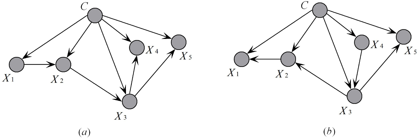
As a one-dependence Bayesian classifier, TAN is optimal. Different attribute orders provide the same undirected Bayesian network, which is the basis of TAN. When a different attribute is selected as the root node, the direction of some arcs may reverse. For example, Figure 3a,b represents the same dependence relationship while X₁ and X₄ are selected as the root nodes, respectively. Additionally, corresponding chain rules are described as:

$$P(x_1,\cdots ,x_5,c)=P(c)P(x_1|c)P(x_2|x_1,c)P(x_3|x_2,c)P(x_4|x_3,c)P(x_5|x_3,c)$$

(13)

and:

$$P(x_1,\cdots ,x_5,c)=P(c)P(x_4|c)P(x_3|x_4,c)P(x_2|x_3,c)P(x_1|x_2,c)P(x_5|x_3,c)$$

(14)

Sum_MI is the same for Figure 3a, b. That is the main reason why TAN performs almost the same, while the causal relationships implicated in the network structure differ. To achieve diversity, Ma and Shi [21] proposed the RTAN algorithm, the output of which is TAN ensembles. Each sub-classifier is trained with different training subsets sampled from the original instances, and the final decision is generated by a majority of votes.

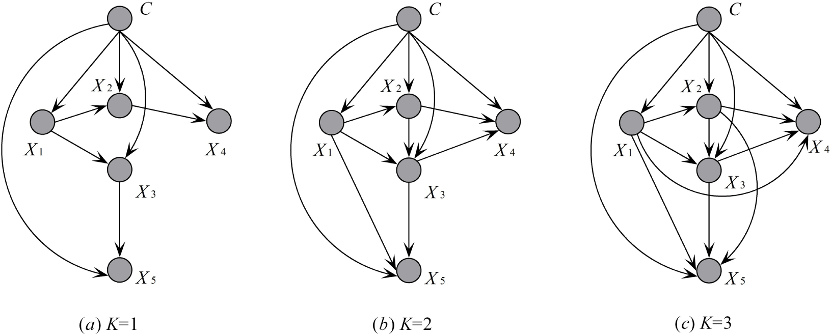
KDB: In KDB, the probability of each attribute value is conditioned by the class variable and, at most, K predictive attributes. The KDB algorithm adopts a greedy strategy in order to identify the graphical structure of the resulting classifier. KDB sets the order of attributes by calculating mutual information and achieves the weights of the relationship between attributes by calculating conditional mutual information. For example, given five predictive attributes {X₁, X₂, X₃, X₄, X₅} and supposing that I(X₁;C) > I(X₂; C) > I(X₃;C) > I(X₄; C) > I(X₅; C), the attribute order is {X₁, X₂, X₃, X₄, X₅} by comparing mutual information.

From the chain rule of joint probability distribution, there will be:

$$P(c,\mathbf{x})=P(c)P(x_1|c)P(x_2|c,x_1)P(x_3|c,x_1,x_2)P(x_4|c,x_2,x_3,x_1)P(x_5|c,x_3,x_1,x_2,x_4)$$

(15)

Obviously, with more attributes to be considered as possible parent attributes, more causal relationships will be represented, and Sum_MI will be larger correspondingly. However, because of the time and space complexity overhead, only a limited number of attributes will be considered. For KDB, each predictive attribute can select at most K attributes as parent attributes. Figure 4 gives an example to show corresponding KDB models when given different K values.

In summary, from the viewpoint of probability theory, all of these algorithms can be regarded as different variations of the chain rule. Different algorithms tried to get different levels of tradeoff between computational complexity and classification accuracy. One advantage of NB is avoiding model selection, because selecting between alternative models can be expected to increase variance and allow a learning system to overfit the training data. However, the conditional independence assumption makes NB neglect the conditional mutual information between predictive attributes. Thus, NB is zero-dependence based and performs the worst among the three algorithms. TAN proposes to achieve global optimization by building MST to weigh the one-dependence causal relationships, i.e., TAN can only have at most one parent, except the class variable. Thus, only a limited number of dependencies or a limited information quantity can be represented in TAN. KDB allows for higher dependence to represent much more complicated relationships between attributes and can have at most K parent attributes. However, KDB is guided by a rigid ordering obtained by using the mutual information between the predictive attribute and the class variable. Mutual information does not consider the interaction between predictive attributes, and this marginal knowledge may result in sub-optimal order. Suppose K = 2 and I(C; X₁) > I(C; X₂) > I(C; X₃) > I(C; X₄) > I(C; X₅); X₃ will use X₂ as the parent attribute, even if they are independent of each other. When K = 1, KDB performs poorer than TAN, because it can only achieve a local optimal network structure. Besides, as described in Equation (9)I(X_i; X_j|C) can only partially measure the dependence between X_i and {X_j, C}.

4. The Flexible K-Dependence Bayesian Classifier

To retain the privileges of TAN and KDB, i.e., global optimization and higher dependence representation, we presently give an algorithm, i.e., FKDB, which also allows one to construct K-dependence classifiers along the attribute dependence spectrum. To achieve the optimal attribute order, FKDB considers not only the dependence between the predictive attribute and the class variable, but also the dependencies among predictive attributes. As the learning procedure proceeds, the attributes will be put into order one by one. Thus, the order is determined dynamically.

Let S represent the attribute set, and predictive attributes will be added to S in a sequential order. The newly-added attribute X_j must select parent attributes from S. To achieve global optimization, X_j should have the strongest relationship with its parent attributes on average, i.e., the largest mutual information should be between X_j and {Pa_j,C}. Once selected, X_j will be added to S as possible parent attributes of the following attribute. FKDB applies greedy search of the mutual information space to find an optimal ordering of all of the attributes, which may help to fully describe the interaction between attributes.

Algorithm 1 is described as follows:

Algorithm 1. Algorithm FKDB.

Input: a database of pre-classified instances, DB, and the K value for the maximum allowable degree of attribute dependence.

Output: a K-dependence Bayesian classifiers with conditional probability tables determined from the input data.

Let the used attribute list, S, be empty. Select attribute Xroot that corresponds to the largest value I(Xi; C), and add it to S. Add an arc from C to Xroot. Repeat until S includes all domain attributes • Select attribute Xi, which is not in S and corresponds to the largest sum value: $$I(X_i;C)+{\displaystyle \sum _{j=1}^{q}I(X_i,X_j|C),}$$ where Xj ∈ S and q = min(|S|; K). • Add a node to BN representing Xi. • Add an arc from C to Xi in BN. • Add q arcs from q distinct attributes Xj in S to Xi. • Add Xi to S. Compute the conditional probability tables inferred by the structure of BN using counts from DB, and output BN.

Algorithm 1. Algorithm FKDB.

Input: a database of pre-classified instances, DB, and the K value for the maximum allowable degree of attribute dependence.

Output: a K-dependence Bayesian classifiers with conditional probability tables determined from the input data.

Let the used attribute list, S, be empty. Select attribute Xroot that corresponds to the largest value I(Xi; C), and add it to S. Add an arc from C to Xroot. Repeat until S includes all domain attributes • Select attribute Xi, which is not in S and corresponds to the largest sum value: $$I(X_i;C)+{\displaystyle \sum _{j=1}^{q}I(X_i,X_j|C),}$$ where Xj ∈ S and q = min(|S|; K). • Add a node to BN representing Xi. • Add an arc from C to Xi in BN. • Add q arcs from q distinct attributes Xj in S to Xi. • Add Xi to S. Compute the conditional probability tables inferred by the structure of BN using counts from DB, and output BN.

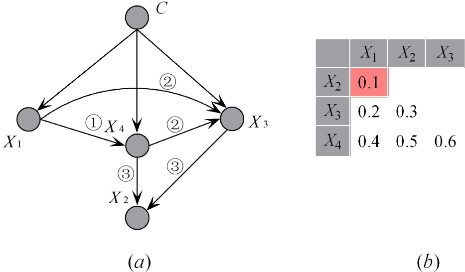
FKDB requires that at most K parent attributes can be selected for each new attribute. To make the working mechanism of FKDB clear, we set K = 2 in the following discussion. Because I(X_i; X_j|C) = I(X_j; X_i|C), we describe the relationships between attributes using an upper triangular matrix of conditional mutual information. 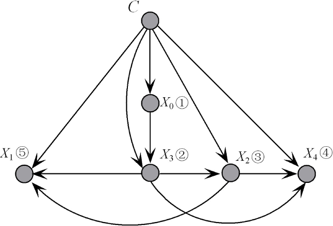The format and one example with five predictive attributes {X₀,X₁,X₂,X₃,X₄} are shown in Figure 5a,b, respectively. Suppose that I(X₀; C) > I(X₃;C) > I(X₂; C) > I(X₄; C) > I(X₁; C), X₀ is added into S as the root node. X₃ = argmax (I(X_i; C) + I(X₀; X_i|C)) (X_i ∉ S); thus, X₃ is added to S; and S = {X₀, X₃}. X₂ = argmax (I(X_i; C) + I(X₀; X_i|C) + I(X₃; X_i|C)) (X_i ∉ S); thus, X₂ is added into S; and S = {X₀,X₂,X₃}. Similarly, X₄ = argmax (I(X_i; C) + I(X_j,X_i|C) + I(X_k, X_i|C)) (X_i ∉ S, X_j, X_k ∈ S); thus, X₄ is added into S, and X₁ will be the last one in the order. Thus, the whole attribute order and causal relationship can be achieved simultaneously. The final network structures is illustrated in Figure 6.

Optimal attribute order and high dependence representation are two key points for learning KDB. Note that KDB achieves these two goals in different steps. KDB first computes and compares mutual information to get an attribute order before structured learning. Then, during the structured learning procedure, each predictive attribute X_i can select at most K attributes as parent attributes by comparing conditional mutual information (CMI). Because these two steps are separate, the attribute order cannot ensure that the first K strongest dependencies between X_i and other attributes should be represented. On the other hand, to achieve the optimal attribute order, FKDB considers not only the dependence between predictive attribute and class variable, but also the dependencies among predictive attributes. As the learning procedure proceeds, the attributes will be put into order one by one. Thus, the order is determined dynamically. That is why the classifier is named “flexible”.

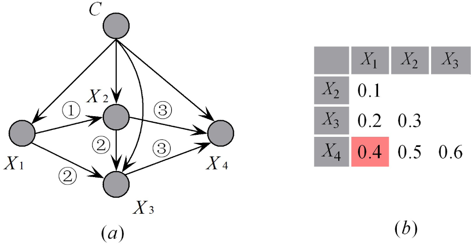
We will further compare KDB and FKDB with an example. Suppose that for KDB, the attribute order is {X₁, X₂, X₃, X₄}; Figure 7 shows the corresponding network structure of KDB when K = 2 corresponds to the CMI matrix shown in Figure 7b, and the learning steps are annotated. The weight of dependencies between attributes are depicted in Figure 7b. Although the dependence relationship between X₂ and X₁ is the weakest, X₁ is selected as the parent attribute of X₂; whereas the strong dependence between X₄ and X₁ is neglected. Suppose that for FKDB, the mutual information I(X_i; C) is the same for all predictive attributes. Figure 8a shows the network structure of FKDB corresponding to the CMI matrix shown in Figure 8b, and learning steps are also annotated. The weights of causal relationships are depicted in Figure 8b, from which we can see that all strong causal relationships are implicated in the final network structure.

5. Experimental Study

In order to verify the efficiency and effectiveness of the proposed FKDB (K = 2), we conduct experiments on 45 datasets from the UCI machine learning repository.

Table 1. Datasets.

No.	Dataset	# Instance	Attribute	Class
1	Lung Cancer	32	56	3
2	Zoo	101	16	7
3	Echocardiogram	131	6	2
4	Hepatitis	155	19	2
5	Glass Identification	214	9	3
6	Audio	226	69	24
7	Hungarian	294	13	2
8	Heart Disease	303	13	2
9	Haberman’s Survival	306	3	2
10	Primary Tumor	339	17	22
11	LiveDisorder (Bupa)	345	6	2
12	Chess	551	39	2
13	Syncon	600	60	6
14	Balance Scale (Wisconsin)	625	4	3
15	Soybean	683	35	19
16	Credit Screening	690	15	2
17	Breast-cancer-w	699	9	2
18	Pima-ind-diabetes	768	8	2
19	Vehicle	846	18	4
20	Anneal	898	38	6
21	Vovel	990	13	11
22	German	1000	20	2
23	LED	1000	7	10
24	Contraceptive Method Choice	1473	9	3
25	Yeast	1484	8	10
26	Volcanoes	1520	3	4
27	Car	1728	6	4
28	Hypothyroid	3163	25	2
29	Abalone	4177	8	3
30	Spambase	4601	57	2
31	Optdigits	5620	64	10
32	Satellite	6435	36	6
33	Mushroom	8124	22	2
34	Thyroid	9169	29	20
35	Sign	12,546	8	3
36	Nursery	12,960	8	5
37	Magic	19,020	10	2
38	Letter-recog	20,000	16	26
39	Adult	48,842	14	2
40	Shuttle	58,000	9	7
41	Connect-4 Opening	67,557	42	3
42	Waveform	100,000	21	3
43	Localization	164,860	5	11
44	Census-income	299,285	41	2
45	Poker-hand	1,025,010	10	10

summarizes the characteristics of each dataset, including the numbers of instances, attributes and classes. Missing values for qualitative attributes are replaced with modes, and those for quantitative attributes are replaced with means from the training data. For each benchmark dataset, numeric attributes are discretized using MDL discretization [22]. The following algorithms are compared:

• NB, standard naive Bayes.
• TAN [23], tree-augmented naive Bayes applying incremental learning.
• RTAN [21], tree-augmented naive Bayes ensembles.
• KDB (K = 2), standard K-dependence Bayesian classifier.

All algorithms were coded in MATLAB 7.0 (MathWorks, Natick, MA, USA) on a Pentium 2.93 GHz/1 G RAM computer. Base probability estimates P(c), P(c, xi) and P(c, x_i, x_j) were smoothed using the Laplace estimate, which can be described as follows:

$$\{\begin{array}{l}\widehat{P}(c)=\frac{F(c)+1}{M+m}\\ \widehat{P}(c,x_i)=\frac{F(c,x_i)+1}{M_i+m_i}\\ \widehat{P}(c,x_i,x_j)=\frac{F(c,x_i,x_j)+1}{M_{ij}+m_{ij}}\end{array}$$

(16)

where F(·) is the frequency with which a combination of terms appears in the training data, M is the number of training instances for which the class value is known, M_i is the number of training instances for which both the class and attribute X_i are known and M_ij is the number of training instances for which all of the class and attributes X_i and X_j are known. m is the number of attribute values of class C; mi is the number of attribute value combinations of C and X_i; and m_ij is the number of attribute value combinations of C, Xj and X_i.

In the following experimental study, functional dependencies (FDs) [24] are used to detect redundant attribute values and to improve model interpretability. To maintain the K-dependence restriction, P(x_i|x₁, ⋯, x_k, c) will be used as an approximate estimation of P(x_i|x₁, ⋯, x_i–1, c) when i > K. Obviously, P(x_i|x₁, ⋯, x_k+1, c) will be more accurate than P(x_i|x_1, ⋯, x_k, c). If there exists FD:x₂ → x₁, then x₂ functionally determines x₁ and x₁ is extraneous for classification. According to the augmentation rule of probability [24],

$$P(x_i|x_1,\cdots ,x_{K+1,}c)=P(x_i|x_2,\cdots ,x_{K+1,}c).$$

Correspondingly, in practice, FKDB uses P(x_i|x₂, ⋯ ,x_k+1, c) instead, which still maintains K-dependence restriction, whereas it represents more causal relationships.

FDs use the following criterion:

$$Count(x_i)=Count(x_i,x_j)\ge l$$

to infer that x_i → x_j, where Count(xi) is the number of training cases with value x_i, Count(x_i, x_j) is the number of training cases with both values and l is a user-specified minimum frequency. A large number of deterministic attributes, which are on the left side of the FD, will increase the risk of incorrect inference and, at the same time, needs more computer memory to store credible FDs. Consequently, only the one-one FDs are selected in our current work. Besides, as no formal method has been used to select an appropriate value for l, we use the setting that l = 100, which is achieved from empirical studies.

Kohavi and Wolpert [25] presented a powerful tool from sampling theory statistics for analyzing supervised learning scenarios. Suppose c and c are the true class label and that generated by classifier A, respectively, for the i-th testing sample; the zero-one loss is defined as:

$${\xi }_i(A)=1-\delta (c,\widehat{c})$$

where δ(c, ĉ) = 1 if ĉ = c and 0 otherwise.

Table 2. Experimental results of zero-one loss.

Dataset	NB	TAN	RTAN	KDB	FKDB
Lung Cancer	0.438 ± 0.268	0.594 ± 0.226	0.480 ± 0.319	0.594 ± 0.328	0.688 ± 0.238
Zoo	0.029 ± 0.047	0.010 ± 0.053	0.029 ± 0.050	0.050 ± 0.052	0.028 ± 0.047
Echocardiogram	0.336 ± 0.121	0.328 ± 0.107	0.308 ± 0.101	0.344 ± 0.067	0.320 ± 0.072
Hepatitis	0.194 ± 0.100	0.168 ± 0.087	0.173 ± 0.090	0.187 ± 0.092	0.170 ± 0.089
Glass Identification	0.262 ± 0.079	0.220 ± 0.083	0.242 ± 0.087	0.220 ± 0.086	0.201 ± 0.079
Audio	0.239 ± 0.055	0.292 ± 0.093	0.195 ± 0.091	0.323 ± 0.088	0.358 ± 0.073
Hungarian	0.160 ± 0.069	0.170 ± 0.063	0.160 ± 0.079	0.180 ± 0.088	0.177 ± 0.081
Heart Disease	0.178 ± 0.069	0.193 ± 0.092	0.164 ± 0.073	0.211 ± 0.083	0.164 ± 0.079
Haberman’s Survival	0.281 ± 0.101	0.281 ± 0.100	0.270 ± 0.097	0.281 ± 0.103	0.281 ± 0.092
Primary Tumor	0.546 ± 0.091	0.543 ± 0.100	0.552 ± 0.094	0.572 ± 0.091	0.590 ± 0.089
Live Disorder(Bupa)	0.444 ± 0.078	0.444 ± 0.017	0.426 ± 0.037	0.444 ± 0.046	0.443 ± 0.067
Chess	0.113 ± 0.055	0.093 ± 0.049	0.096 ± 0.045	0.100 ± 0.054	0.076 ± 0.048
Syncon	0.028 ± 0.033	0.008 ± 0.015	0.010 ± 0.025	0.013 ± 0.022	0.011 ± 0.019
Balance Scale	0.285 ± 0.025	0.280 ± 0.022	0.286 ± 0.026	0.278 ± 0.028	0.280 ± 0.021
Soybean	0.089 ± 0.024	0.047 ± 0.014	0.045 ± 0.014	0.056 ± 0.013	0.051 ± 0.021
Credit Screening	0.141 ± 0.033	0.151 ± 0.048	0.134 ± 0.037	0.146 ± 0.051	0.149 ± 0.042
Breast-cancer-w	0.026 ± 0.022	0.042 ± 0.048	0.034 ± 0.032	0.074 ± 0.025	0.080 ± 0.039
Pima-ind-diabetes	0.245 ± 0.075	0.238 ± 0.062	0.229 ± 0.065	0.245 ± 0.113	0.247 ± 0.089
Vehicle	0.392 ± 0.059	0.294 ± 0.056	0.278 ± 0.060	0.294 ± 0.061	0.299 ± 0.056
Anneal	0.038 ± 0.343	0.009 ± 0.376	0.009 ± 0.350	0.009 ± 0.281	0.008 ± 0.296
Vowel	0.424 ± 0.056	0.130 ± 0.046	0.144 ± 0.036	0.182 ± 0.026	0.150 ± 0.041
German	0.253 ± 0.034	0.273 ± 0.062	0.238 ± 0.044	0.289 ± 0.068	0.284 ± 0.052
LED	0.267 ± 0.062	0.266 ± 0.057	0.258 ± 0.052	0.262 ± 0.052	0.272 ± 0.060
Contraceptive Method	0.504 ± 0.038	0.489 ± 0.023	0.474 ± 0.028	0.500 ± 0.038	0.488 ± 0.030
Yeast	0.424 ± 0.031	0.417 ± 0.037	0.407 ± 0.032	0.439 ± 0.031	0.438 ± 0.034
Volcanoes	0.332 ± 0.029	0.332 ± 0.030	0.318 ± 0.024	0.332 ± 0.024	0.338 ± 0.027
Car	0.140 ± 0.026	0.057 ± 0.018	0.078 ± 0.022	0.038 ± 0.012	0.046 ± 0.018
Hyprothyroid	0.015 ± 0.004	0.010 ± 0.005	0.013 ± 0.004	0.011 ± 0.012	0.010 ± 0.008
Abalone	0.472 ± 0.024	0.459 ± 0.025	0.450 ± 0.024	0.467 ± 0.028	0.467 ± 0.024
Spambase	0.102 ± 0.013	0.067 ± 0.010	0.066 ± 0.010	0.064 ± 0.014	0.065 ± 0.011
Optdigits	0.077 ± 0.009	0.041 ± 0.008	0.040 ± 0.007	0.037 ± 0.010	0.031 ± 0.009
Satellite	0.181 ± 0.016	0.121 ± 0.011	0.119 ± 0.015	0.108 ± 0.014	0.115 ± 0.012
Mushroom	0.020 ± 0.004	0.000 ± 0.008	0.000 ± 0.004	0.000 ± 0.000	0.000 ± 0.001
Thyroid	0.111 ± 0.010	0.072 ± 0.005	0.071 ± 0.007	0.071 ± 0.006	0.069 ± 0.008
Sign	0.359 ± 0.007	0.276 ± 0.010	0.270 ± 0.008	0.254 ± 0.006	0.223 ± 0.007
Nursery	0.097 ± 0.006	0.065 ± 0.008	0.064 ± 0.006	0.029 ± 0.006	0.028 ± 0.006
Magic	0.224 ± 0.006	0.168 ± 0.004	0.165 ± 0.009	0.157 ± 0.011	0.160 ± 0.006
Letter-recog	0.253 ± 0.008	0.130 ± 0.007	0.127 ± 0.008	0.099 ± 0.007	0.081 ± 0.005
Adult	0.158 ± 0.004	0.138 ± 0.003	0.135 ± 0.004	0.138 ± 0.004	0.132 ± 0.003
Shuttle	0.004 ± 0.001	0.002 ± 0.001	0.001 ± 0.001	0.001 ± 0.001	0.001 ± 0.001
Connect-4 Opening	0.278 ± 0.006	0.235 ± 0.005	0.231 ± 0.004	0.228 ± 0.004	0.218 ± 0.005
Waveform	0.022 ± 0.002	0.020 ± 0.001	0.020 ± 0.002	0.026 ± 0.002	0.018 ± 0.010
Localization	0.496 ± 0.003	0.358 ± 0.002	0.350 ± 0.003	0.296 ± 0.003	0.280 ± 0.001
Census-income	0.237 ± 0.002	0.064 ± 0.002	0.063 ± 0.002	0.051 ± 0.002	0.051 ± 0.002
Poker-hand	0.499 ± 0.002	0.330 ± 0.002	0.333 ± 0.002	0.196 ± 0.002	0.192 ± 0.002

presents for each dataset the zero-one loss and the standard deviation, which are estimated by 10-fold cross-validation to give an accurate estimation of the average performance of an algorithm. Statistically, a win/draw/loss record (W/D/L) is calculated for each pair of competitors A and B with regard to a performance measure M. The record represents the number of datasets in which A respectively beats, loses to or ties with B on M. Small improvements may be attributable to chance. Runs with the various algorithms are carried out on the same training sets and evaluated on the same test sets. In particular, the cross-validation folds are the same for all of the experiments on each dataset. Finally, related algorithms are compared via a one-tailed binomial sign test with a 95 percent confidence level.

Table 3. Win/draw/loss record (W/D/L) comparison results of zero-one loss on all datasets.

W/D/L	NB	TAN	RTAN	KDB
TAN	27/11/7
RTAN	29/13/3	10/27/8
KDB	24/13/8	12/20/13	15/12/18
FKDB	26/11/8	16/20/9	15/15/15	12/28/5

shows the W/D/L records corresponding to zero-one loss. When dependence complexity increases, the performance of TAN gets better than that of NB. RTAN investigates the diversity of TAN by the K statistic. The bagging mechanism helps RTAN to achieve superior performance to TAN. FKDB performs undoubtedly the best. However, surprisingly, as a 2-dependence Bayesian classifier, the advantage of KDB is not obvious when compared to 1-dependence classifiers, and it even performs poorer than RTAN in general. However, when the data size increases to a certain extent, e.g., 4177 (the size of dataset “Abalone”), as

Table 4. Win/draw/loss record (W/D/L) comparison results of zero-one loss when the data size > 4177.

W/D/L	NB	TAN	RTAN	KDB
TAN	16/1/0
RTAN	16/1/0	0/17/0
KDB	15/1/1	11/5/1	10/6/1
FKDB	16/1/0	11/6/0	10/7/0	4/12/1

shows, the prediction performance of all restricted classifiers can be evaluated from the perspective of the dependence level. Two-dependence Bayesian classifiers, e.g., FKDB and KDB, perform the best. The one-dependence Bayesian classifier, e.g., TAN, performs better. Additionally, 0-dependence Bayesian classifiers, e.g., NB, perform the worst.

Friedman proposed a non-parametric measure [28], the Friedman test, which compares the ranks of the algorithms for each dataset separately. The null-hypothesis is that all of the algorithms are equivalent, and there is no difference in average ranks. We can compute the Friedman statistic:

$$F_r=\frac{12}{Nt(t+1)}{\displaystyle \sum _{j=1}^t{R}_j^2-3N(t+1)}$$

by using the chi-square distribution with t – 1 degrees of freedom, where $R_j={\displaystyle {\sum }_i{r}_i^j}$ and $r_i^j$ is the rank of the j-th of t algorithms on the i-th of N datasets. Thus, for any selected level of significance α, we reject the null hypothesis if the computed value of F_r is greater than ${\chi }_{\alpha }^2$, the upper-tail critical value for the chi-square distribution having t – 1 degrees of freedom. The critical value of ${\chi }_{\alpha }^2$ for α = 0.05 is 1.8039. The Friedman statistic for 45 datasets and 17 large (size > 4177) datasets are 12 and 28.9, respectively. Additionally, p < 0.001 for both cases. Hence, we reject the null-hypotheses.

The average ranks of zero-one loss of different classifiers on all and large datasets are {NB(3.978), TAN(2.778), RTAN(2.467), KDB(3.078), FKDB(2.811)} and {NB(4.853), TAN(3.118), RTAN(3), KDB(2.176) and FKDB(2)}, respectively. Correspondingly, the order of these algorithms is {RTAN, TAN, FKDB, KDB, NB} when comparing the experimental results on all datasets. The performance of FKDB is not obviously superior to other algorithms. However, when comparing the experimental results on large datasets, the order changes greatly and turns out to be {FKDB, KDB, RTAN, TAN, NB}.

When the class distribution is imbalanced, traditional classifiers are easily overwhelmed by instances from majority classes, while the minority classes instances are usually ignored [26]. A classification system should, in general, work well for all possible class distribution and misclassification costs. This issue was successfully addressed in binary problems using ROC analysis and the area under the ROC curve (AUC) metric [27]. Research on related topics, such as imbalanced learning problems, is highly focused on the binary class problem, while progress on multiclass problems is limited [26]. Therefore, we select 16 datasets with binary class labels for comparison of the AUC. The AUC values are shown in

Table 5. Experimental results of the average AUCs for datasets with binary class labels.

Dataset	NB	TAN	RTAN	KDB	FKDB
Adult	0.920	0.928	0.931	0.941	0.935
Breast-cancer-w	0.992	1.000	1.000	1.000	1.000
Census-income	0.960	0.989	0.991	0.992	0.993
Chess	0.957	0.986	0.992	0.988	0.993
Credit Screening	0.932	0.963	0.956	0.978	0.967
Echocardiogram	0.737	0.771	0.775	0.771	0.776
German	0.814	0.877	0.893	0.941	0.929
Haberman’s Survival	0.659	0.658	0.687	0.657	0.692
Heart Disease	0.922	0.936	0.946	0.956	0.951
Hepatitis	0.929	0.968	0.983	0.985	0.977
Hungarian	0.931	0.957	0.961	0.964	0.962
Live Disorder(Bupa)	0.620	0.620	0.620	0.620	0.620
Magic	0.866	0.905	0.902	0.916	0.911
Mushroom	0.999	1.000	1.000	1.000	1.000
Pima-ind-diabetes	0.851	0.865	0.866	0.876	0.877
Spambase	0.966	0.980	0.987	0.989	0.985

. With 5 algorithms and 16 datasets, the Friedman statistic F_r = 2.973 and p < 0.004. Hence, we reject the null-hypotheses again. The average ranks of different classifiers are {NB(3.6), TAN(3.0), RTAN(2.833), KDB(2.867) and FKDB(2.7)}. Hence, the order of these algorithms is {FKDB, RTAN, KDB, TAN, NB}. The effectiveness of FKDB is proven from the perspectives of AUC.

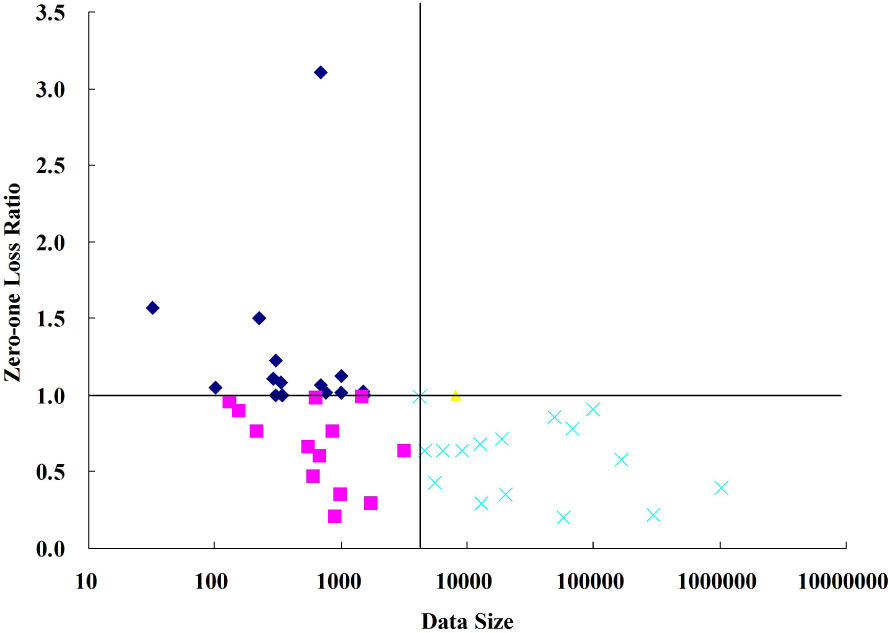
To compare the relative performance of classifiers A and B, the zero-one loss ratio (ZLR) is proposed in this paper and defined as ZLR(A/B) = ∑ ξ_i (A)/∑ξ_i(B). Figures 9–12 compare FKDB with NB, TAN, RTAN and KDB, respectively. Each figure is divided into four parts by comparing data size and ZLR. That is, the data size is greater than 4177 while ZLR ≥ 1 or ZLR < 1, and the data size is smaller than 4177 while ZLR ≥ 1 or ZLR < 1. In different parts, different symbols are used to represent different situations. When dealing with small datasets (data size <4177), the performance superiority of FKDB is not obvious when compared to the 0-dependence (NB) or 1-dependence Bayesian classifiers (TAN). For some datasets, e.g., “Lung Cancer” and “Hungarian”, NB even performs the best. Because precise estimation of conditional mutual information is determined by probability estimation, which is affected greatly by data size, the robustness of network structure will be affected negatively by imprecise probability estimation. For example, for dataset “Lung Cancer” with 32 instances and 56 attributes, it is almost impossible to ensure that the basic causal relationships learned are of a high confidence level. That is why a simple structure can perform better than a complicated one. Since each submodel of RTAN can represent only a small proportion of all dependencies, the complementarity of the bagging mechanism works and helps to improve the performance of TAN. KDB shows equivalent performance to FKDB.

As data size increases, high-dependence Bayesian classifiers gradually show their superiority, and the advantage of FKDB is almost overwhelming when compared to NB and TAN. Because almost all strong dependencies can be detected and illustrated in each submodel of RTAN, the high degree of uniformity in the basic structure cannot help to improve the prediction performance of TAN. Thus, RTAN shows equivalent performance to TAN. The prediction superiority of FKDB over KDB becomes much more obvious. Because they both are 2-dependence Bayesian classifiers, a minor difference in local structure may be the main cause of the performance difference. To further clarify this idea, we propose a new criterion, Info_ratio(A/B), to compare the information quantity implicated in Bayesian classifiers A and B.

$$\mathit{\text{Info\_ratio}}(A/B)=\mathit{\text{Sum\_MI}}(A)/\mathit{\text{Sum\_MI}}(B)$$

(17)

The comparison results of Info_ratio(FKDB/KDB) are shown in Figure 13, from which the superiority of FKDB in extracting information is much more obvious when dealing with large datasets. The increased information quantity does help to decrease zero-one loss. However, note that the growth rate of information quantity is not in proportion to the descent rate of zero-one loss. For some datasets, e.g., “Localization” and “Poker-hand”, KDB and FKDB achieve the same Sum_MI, while their zero-one losses are different. The same Sum_MI corresponds to the same causal relationships. The network structures learned from KDB and FKDB are similar, because the major dependencies are all implicated, except that the directions of some arcs are different. Dependence “X₃ – X₄” can be represented by conditional probability distribution P(x₃|x₄, c) or P(x₄|x₃, c). Just as we clarified in Section 3, although the basic structures described in Figure 3a,b are the same, the corresponding joint probability distributions represented by Equations (13) and (14) are different. Since ZLR ≈ 1 for these two datasets, the difference in zero-one loss can be explained from the perspective of probability distribution.

To prove the relevance of information quantity to zero-one loss, Figure 14 is divided into four zones. Similar to the comparison of Equations (13) and (14), the same information quantity does not certainly correspond to the same Bayesian network and, then, the same zero-one loss. Zone A contains 27 datasets and describes the situation that ZLR<1 and Info_ratio ≥ 1. The performance superiority of FKDB over KDB can be attributed to mining more information or correct conditional dependence representation. Zone D contains 6 datasets and describes the situation that ZLR>1 and Info_ratio ≤ 1. The performance inferiority of FKDB over KDB can be attributed to mining less information. Thus, the information quantity is strongly correlated to zero-one loss on 73.3% $(\frac{27+6}{45})$ of all datasets. On the other hand, although FKDB has proven its effectiveness from the perspective of W/D/L results and the Friedman test, the information quantity is a very important score, but not the only one.

6. Conclusions

BNs can graphically describe conditional dependence between attributes, and they have been previously demonstrated to be computationally efficient approaches to further reducing zero-one loss. Conditional mutual information is commonly applied to weigh the dependencies between attributes, while it cannot measure the information quantity provided to predictive attributes. On the basis of analyzing and summarizing the working mechanisms of three popular Bayesian classifiers from the viewpoints of information theory and probability theory, this paper proposed to mine reliable dependencies by maximizing the sum of mutual information. The experimental results validate the mapping relationship between conditional probability distribution and mutual information.