An Entropy-Based Approach to Path Analysis of Structural Generalized Linear Models: A Basic Idea

Path analysis [1] is often applied to causal systems of continuous variables through the linear structural equations model (LISREL) [2,3]. In the LISREL approach, causal relationships among variables are described by a path diagram and translated into linear equations of the variables. Causal effects can then be calculated by regression and correlation coefficients obtained for the linear equations. In contrast, path analysis of categorical variables is more complex than that of continuous variables because the causal system under consideration cannot be described by linear regression equations. Goodman [4–7] considered path analysis of binary variables by using logit models and discussed the effects of explanatory variables, though without discussing direct and indirect effects. Hagenaars [8] discussed path analysis of categorical variables by using a log-linear model, but here as well without discussion of direct and indirect effects. Eshima et al. [9] proposed a path analysis method for categorical variables in logit models. Kuha and Goldthorpe [10] gave a two-stage path analysis method for generalized linear models (GLMs) that uses log odds ratios. In their approach, first the total, direct and indirect effects are defined for mean differences of response variables, and then the method is applied to measuring the effects on the basis of log odds ratios. However, additive decomposition of the total effect into the direct and indirect effects only approximately reflects reality, and assessing effects in categorical (polytomous) variable systems become more complicated as the numbers of variable categories are increased [10]. Albert and Nelson [11] proposed a path analysis method to calculate pathway effects for causal systems on the basis of GLMs, but not all pathway effects are identifiable. As in the two-stage cases, when factors, intermediate variables, and response variables are categorical, pathway effects become very complicated because the variable effects are defined for mean differences of response variables.

There are many examples of response variables in practical data that are not normally distributed in various fields of study. There is need for a method of path analysis with responses that are not normally distributed, especially categorical responses, and it is useful to discuss a path analysis approach for causal systems of GLMs [12,13]. When describing causal systems of the variables by GLMs, regression parameters or coefficients are related to log odds ratios [14–16], and so it is natural to consider the effects of factors (explanatory variables) according to odds or log odds ratios. However results become more complicated as the number of categories of the variables increases. In such cases, it is suitable to summarize the effects of factors in GLMs. For this purpose, we use the entropy coefficient of determination (ECD), one of the entropy-based measures of predictive power for GLMs [15,16].

The remainder of this paper is organized as follows: Section 2 presents a practical example of causal systems—British mobility data [10]—and re-analyzes them by a new method of path analysis. Section 3 considers the relation between the log odds ratio and entropy, and ECD is briefly reviewed. Section 4 introduces a path analysis method for causal systems described by GLMs, and in Section 5 a method for testing effects of variables is given. The British mobility data are re-analyzed by the proposed approach in Section 6. Finally, Section 7 provides some discussion and conclusions for the present approach.

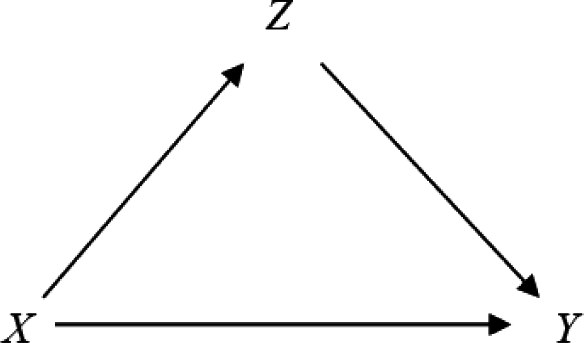
British mobility data describe the effects of education on social class mobility [10]. There are three variables, which are causally ordered as shown in Figure 1: parents’ social class, X; individual social class, Y; and education, Z, which intermediates between X and Y. The three variables are discrete. Social classes X and Y have three categories, “salariat and employers”, “middle class”, and “working class”; education Z has seven levels. While the effects of X and Z on Y can be discussed through log odds ratios, the results are complicated because the number of variable categories is large. It is important to summarize causal effects measured with log odds ratios, especially in such practical examples, to assess the intermediate effect of education on social class mobility.

Let $\mathbf{X}$ and Y be a p × 1 explanatory-variable vector and a response variable, respectively, and let $f\left(y|\mathbf{x}\right)$ be the conditional probability or probability density function of Y given that $\mathbf{X}=\mathbf{x}$. The function $f\left(y|\mathbf{x}\right)$ is assumed to belong to the following family of exponential distributions: where θ and φ are parameters, and $a\left(\varphi \right)$ (>0), $b\left(\theta \right)$, and $c\left(y,\varphi \right)$ are known functions. Let ${\mathbf{\beta }}^T={\left({\beta }_1,{\beta }_2,\mathrm{...},{\beta }_p\right)}^T$. The function θ is a function of $\mathbf{\eta }={\mathbf{\beta }}^T\mathbf{x}$ through a link function $h\left(u\right)$.

Remark 1. In general, the systematic component can be extended to be a function of explanatory variable vector x. Then, the model is referred to as a generalized nonlinear model. For the sake of simplicity, the function is denoted by$\theta =\theta \left(\mathbf{x}\right)$. The discussion below is applicable to this case.

Let ${\mathbf{\mu }}_{\mathbf{X}}$ and ${\mu }_Y$ be the means of $\mathbf{X}$ and $Y$, respectively. Then, let us consider the following log odds ratio:

The first and second terms of the right hand side of the above equation are the relative information with respect to response variable $Y$, so the log odds ratio is the change of the relative information in explanatory variable vector $\mathbf{X}$. In GLMs, taking the expectation of the above log odds ratio with respect to $\mathbf{X}$ and Y, it is reduced to $\frac{\mathrm{cov}\left(\theta ,Y\right)}{a\left(\varphi \right)}$. The quantity $\frac{\mathrm{cov}\left(\theta ,Y\right)}{a\left(\varphi \right)}$ can be expressed as a symmetric type of the Kullback–Leibler (KL) information between a GLM based on (1) and the null model with ${\mathbf{\beta }}^T=0$ [15]; thus, we denote $\frac{\mathrm{cov}\left(\theta ,Y\right)}{a\left(\varphi \right)}$ by $KL\left(\mathbf{X},Y\right)$ in this paper. Let $f\left(y\right)$ be the density or probability function for null model ${\mathbf{\beta }}^T=0$ and let $g\left(\mathbf{x}\right)$ be that of $\mathbf{X}$. Then:

If the variables in the above are discrete, the related integrals are replaced by the summations. The ECD is then defined as:

Then, ECD can also be expressed as:

The measure is interpreted as the proportion of the variation in entropy of Y that is explained by $\mathbf{X}$ [15,16]. As shown above, GLMs explain the entropy of response variables, so it is suitable to measure the effects of explanatory variables based on entropy.

Remark 2. Applying ECD to the linear regression model, ECD is the usual coefficient of determination$R^2$.

For simplicity, in the recursive case with $X_i$$\left(i=1,2,3\right)$, where $X_i$ precedes $X_{i+1}$$\left(i=1,2\right)$, we discuss the effects of $X_1$ and $X_2$ on $X_3$. Let ${\mu }_i$ be the expectation of $X_i$$\left(i=1,2,3\right)$. Then, for a GLM with the conditional density or probability function of $X_3$ when $\left(X_1,X_2\right)=\left(x_1,x_2\right)$ given by (1), the total effect of $\left(X_1,X_2\right)=\left(x_1,x_2\right)$ on $X_3=x_3$ can be defined by using the following log odds ratio:

Taking the expectation of the above effect with respect to $X_1$, $X_2$ and $X_3$, we have:

The above KL information is the (summary) total effect of explanatory variables $\left(X_1,X_2\right)$ on response variable $X_3$. Let ${\mu }_2\left(x_1\right)$ and ${\mu }_3\left(x_1\right)$ be the conditional expectations for $X_2$ and $X_3$, respectively, given that $X_1=x_1$. The log odds ratio with respect to $x_2$ and $x_3$ for a given $x_1$ is:

The total effect of $X_2=x_2$ on $X_3=x_3$ when $X_1=x_1$ is defined by the above log odds ratio because the effect expresses the total effect of $X_2=x_2$ on $X_3=x_3$ when the effect of the preceding variable $X_1=x_1$ is excluded. From this, the total effect of $X_1=x_1$ on $X_3=x_3$ is defined by

By taking the expectation of the above information with respect to $X_1$, $X_2$ and $X_3$, the (summary) total effect of $X_1$ on $X_3$ is given by where $KL\left(X_2,X_3|X_1\right)$ is given by

The second term implies the effect of $X_2$ by itself, that is, the effect of $X_2$ on $X_3$ when the effect of $X_1$ is excluded, and is defined as the (summary) total effect of $X_2$ on $X_3$. The direct effect of $X_1=x_1$ on $X_3=x_3$ can be understood according to the following odds ratio:

The above effect is derived by excluding the effect of $X_2=x_2$, so it is defined as the direct effect of $X_1=x_1$ on $X_3=x_3$. Taking the expectation of the above effect, we have the (summary) direct effect of $X_1$ on $X_3$, expressed as follows: where $KL\left(X_1,X_3|X_2\right)$ is defined as in (2). The above quantity is the amount of entropy of $X_3$ explained by $X_1$ alone, that is, excluding the effect of $X_2$. By subtracting the direct effect of $X_1=x_1$ on $X_3=x_3$ from the total effect, we have the indirect effect of $X_1=x_1$ on $X_3=x_3$:

Taking the expectation of the above effect, the (summary) indirect effect is given by

As in the previous section, to standardize the above effects by ECD, we define the standardized total, direct, and indirect effects of $X_1$ and $X_2$ on $X_3$ as follows:

The total effect of $X_1$ and $X_2$ on $X_3$ is:

The total effect of $X_1$ on $X_3$:

The direct effect of $X_1$ on $X_3$:

The indirect effect of $X_1$ on $X_3$:

The total (direct) effect of $X_2$ on $X_3$:

In this case:

A general approach based on the above discussion is given below. Let $X_i$$\left(i=1,2,\mathrm{..},K\right)$ be variables such that the parents of $X_k$ are ${\mathbf{X}}_{\mathrm{pa}(k)}=\left(X_1{X}_2,\mathrm{...},X_{k-1}\right)$$\left(k=2,3,\mathrm{..},K\right)$, that is, $X_i$ precedes $X_{i+1}$$\left(i=1,2,\mathrm{..},K-1\right)$. Let $f\left(x_K|x_1,x_2,\mathrm{...},x_{K-1}\right)$ be the conditional density or probability of $X_K$ given ${\mathbf{X}}_{\mathrm{pa}(K)}=\left(X_1{X}_2,\mathrm{...},X_{K-1}\right)$ such that:

Explaining response variable $X_K$ in a GLM framework by explanatory variables ${\mathbf{X}}_{\mathrm{pa}(K)}$, the effects of the explanatory variables on the response variable can be treated in terms of entropy as discussed above. From this the standardized (summary) total effect of $X_1$ on $X_K$ is defined by:

Second, the total effect of $X_2$ is defined as:

Then, we can find the total effects of $X_i$ by induction, which yields: where $KL\left(X_{\mathrm{pa}\left(K\right)},X_K|X_{\mathrm{pa}\left(i\right)}\right)$ and $KL\left(X_{\mathrm{pa}\left(K\right)},X_K|X_{\mathrm{pa}\left(i+1\right)}\right)$ can be defined as in (2). In the above formulae, we have: and:

Remark 3. The total effect of$X_i=x_i$ on$X_K=x_K$ is given by: where${\mu }_k\left({\mathbf{x}}_{\mathrm{pa}\left(i\right)}\right)$ and${\mu }_k\left({\mathbf{x}}_{\mathrm{pa}\left(i+1\right)}\right)$ be the conditional expectations of$X_k$ given${\mathbf{X}}_{\mathrm{pa}\left(i\right)}={\mathbf{x}}_{\mathrm{pa}\left(i\right)}$ and${\mathbf{X}}_{\mathrm{pa}\left(i+1\right)}={\mathbf{x}}_{\mathrm{pa}\left(i+1\right)}$, respectively.

Let ${\mathbf{X}}_{\mathrm{pa}\left(K\right)}^{\backslash i}=\left(X_1,X_2,\mathrm{...},X_{i-1},X_{i+1},\mathrm{...},X_{K-1}\right)$ be parent variables of $X_K$ excluding $X_i$. The direct effect of $X_i$ on $X_K$ is defined by:

From this, we have the indirect effect of $X_i$:

Remark 4. The direct effect of$X_i=x_i$ on$X_K=x_K$ is given bywhere${\mu }_i\left({\mathbf{x}}_{\mathrm{pa}\left(K\right)}^{/i}\right)$ is the conditional expectation of$X_i$ given${\mathbf{X}}_{\mathrm{pa}\left(K\right)}^{/i}={\mathbf{x}}_{\mathrm{pa}\left(K\right)}^{/i}$.

For canonical links: we have: and:

From (5) we have:

The direct effect of $X_i$ on $X_K$ is given by: and the indirect effect is calculated by (8) minus (9).

The present approach is different from the usual approach for linear equation models and from the approach in [10], because it is based on the log odds ratio and entropy by using all the variables concerned.

Remark 5. The total effects of variables by Kuha and Goldthorpe [10] are defined with the marginal distributions of response variables and explanatory variables. Meanwhile the present approach defines the total effects of explanatory variables based on a recursive structure of all the variables concerned and we have (6).

Remark 6. Indirect effects are defined by the total effects minus the direct effects as (3), (4) and (7); however the interpretation can be done in terms of entropy. On the other hand, direct and indirect effects are defined in an approach by [10], though the sum of the effects does not equal to the total effect.

Remark 7. Assessing the model identification and testing the goodness-of-fit of the model are based on the discussion of GLMs.

Let $\stackrel{⌢}{K}L\left({\mathbf{X}}_{\mathrm{pa}\left(K\right)},X_K|{\mathbf{X}}_{\mathrm{pa}\left(i\right)}\right),$$\stackrel{⌢}{K}L\left({\mathbf{X}}_{\mathrm{pa}\left(K\right)},X_K|{\mathbf{X}}_{\mathrm{pa}\left(i+1\right)}\right),$ and $\stackrel{⌢}{K}L\left({\mathbf{X}}_{\mathrm{pa}\left(K\right)},X_K|{\mathbf{X}}_{\mathrm{pa}\left(K\right)}^{\backslash i}\right)$ be the ML estimators of $KL\left({\mathbf{X}}_{\mathrm{pa}\left(K\right)},X_K|{\mathbf{X}}_{\mathrm{pa}\left(i\right)}\right),$$KL\left({\mathbf{X}}_{\mathrm{pa}\left(K\right)},X_K|{\mathbf{X}}_{\mathrm{pa}\left(i+1\right)}\right),$ and $KL\left({\mathbf{X}}_{\mathrm{pa}\left(K\right)},X_K|{\mathbf{X}}_{\mathrm{pa}\left(K\right)}^{\backslash i}\right)$, respectively. A similar result presented in Eshima & Tabata [16] can be used to show that: is asymptotically distributed according to a chi-squared distribution with the degrees of freedom equal to the number of parameters in the conditional independent model with ${\mathbf{X}}_{\mathrm{pa}\left(i\right)}$ minus that with ${\mathbf{X}}_{\mathrm{pa}\left(i+1\right)}$.By using statistic (10), the total effects can be tested. Similarly, the statistic: is asymptotically distributed according to a chi-squared distribution with degrees of freedom equal to the number of regression coefficients (parameters) related to variable $X_i$.

The following statistic is asymptotically distributed according to a non-central chi-squared distribution with degree of non-centrality: and an appropriate degrees of freedom ν, found as the number of parameters in the conditional independent model with ${\mathbf{X}}_{\mathrm{pa}\left(i\right)}$ minus that with ${\mathbf{X}}_{\mathrm{pa}\left(i+1\right)}$. Let: and let $c=1+\frac{\lambda }{\nu +\lambda }$ and $\nu \prime =\nu +\frac{{\lambda }^2}{\nu +2\lambda }$. The statistic $\frac{{\chi }_T^2}{c}$ is asymptotically distributed according to the chi-squared distribution with $\nu \prime$ degrees of freedom. As $\nu \prime$ becomes large, the chi-squared distribution tends to a normal distribution with mean $\nu \prime$ and variance $2\nu \prime$. From this, for sufficiently large sample sizes $n$, the statistic: is asymptotically normally distributed with mean $\frac{c\nu \prime }{n}$ and variance $\frac{2c^2\nu \prime }{n^2}$ [17]. For sufficiently large $n$, we have that:

From this, the asymptotic standard error (ASE) of $\frac{{\chi }_T^2}{n}$ is $\frac{2\sqrt{{\chi }_T^2}}{n}$. Similarly, the asymptotic standard error of: is $\frac{2\sqrt{{\chi }_D^2}}{n}$. Moreover: is asymptotically equal to a normal distribution with mean: and variance $\frac{4}{n^2}\left({\chi }_T^2-{\chi }_D^2\right)$. By using the above results, ASEs of the estimates of the summary total and direct effects can be calculated.

The British mobility data described in Section 2 were analyzed in detail by using log odds ratios [10]. Here, the proposed path analysis method is applied to summarize the effects of parental class $X$ and education $Z$ on destination class Y, measured by log odds ratios as in the previous section, and to give a simple interpretation from the summary effects of $X$ and $Z$ on $Y$. The three variables are random, and the GLM system can be composed of logit models. In this example, the employed logistic model can be expressed as follows. Let $X$ be a categorical factor; $Z$ a score that take levels {1,2,3} and {1,2,…,7}, respectively, and let $Y$ be a categorical response variable with levels {1,2,3}. Let:

Then, dummy variable vectors $\mathbf{X}={\left(X_1,X_2,X_3\right)}^T$ and $\mathbf{Y}={\left(Y_1,Y_2,Y_3\right)}^T$ are identified with categorical variables $X$ and response $Y$, respectively. From this, the systematic component of the above model can be expressed as follows: where: