Active Control of a Chaotic Fractional Order Economic System

Abstract

In this paper, a fractional order economic system is studied. An active control technique is applied to control chaos in this system. The stabilization of equilibria is obtained by both theoretical analysis and the simulation result. The numerical simulations, via the improved Adams–Bashforth algorithm, show the effectiveness of the proposed controller.

1. Introduction

Fractional calculus has 300-year history. However, applications of fractional calculus in physics and engineering have just begun. Many systems are known to display fractional order dynamics, such as viscoelastic systems, dielectric polarization and electromagnetic waves [1,2,3,4,5,6]. In recent years, the emergence of effective methods in differentiation and integration of non-integer order equations makes fractional order systems more and more attractive for the systems control community [7,8,9,10].

More recently, there has been a new trend to investigate the control and the dynamic behavior of fractional order chaotic systems. It has been shown that nonlinear chaotic systems may keep their chaotic behavior when their models become fractional [11,12,13].

In this paper, the aim is to control a chaotic fractional-order economic system, using a nonlinear active control method.

This paper is organized as follows: Some preliminaries about fractional calculus, the stability criterion and the numerical algorithm are given in Section 2. The fractional order economic system and its dynamical behavior are described in Section 3. The active control method and the numerical simulations are presented in Section 4. Concluding remarks are drawn in Section 5.

2. Preliminary Tools

2.1. Fractional Calculus

Historical introductions on fractional-order differential equations (FDEs) can be found in [3,4,5,6,14]. Commonly-used definitions for fractional derivatives are due to Riemann–Liouville and Caputo [15]. In what follows, Caputo derivatives are considered, taking the advantage that this allows for traditional initial and boundary conditions to be included in the formulation of the considered problem.

Definition 1. A real function $f\left(x\right),x>0$, is said to be in the space $C_{\mu },\mu \in \mathbb{R}$ if there exits a real number $\lambda >\mu$, such that $f\left(x\right)=x^{\lambda }g\left(x\right)$, where $g\left(x\right)\in C[0,\infty )$, and it is said to be in the space $C_{\mu }^m$ if and only if $f^{\left(m\right)}\in C_{\mu }$ for $m\in IN$.

Definition 2. The Riemann–Liouville fractional integral operator of order α of a real function $f\left(x\right)\in C_{\mu },\mu \ge -1$, is defined as:

$$J^{\alpha }f\left(x\right)=\frac{1}{\Gamma \left(\alpha \right)}{\int }_0^x{(x-t)}^{\alpha -1}f\left(t\right)dt,\alpha >0,x>0,$$

(1)

and $J^{0}f\left(x\right)=f\left(x\right).$ The operators $J^{\alpha }$ have some properties, for $\alpha ,\beta \ge 0$ and $\xi \ge -1$:

• $J^{\alpha }{J}^{\beta }f\left(x\right)=J^{\alpha +\beta }f\left(x\right),$
• $J^{\alpha }{J}^{\beta }f\left(x\right)=J^{\beta }{J}^{\alpha }f\left(x\right),$
• $J^{\alpha }{x}^{\xi }=\frac{\Gamma (\xi +1)}{\Gamma (\alpha +\xi +1)}{x}^{\alpha +\xi }$.

Definition 3. The Caputo fractional derivative $D^{\alpha }$ of a function $f\left(x\right)$ of any real number α, such that $m-1<\alpha \le m$, $m\in IN$, for $x>0$ and $f\in C_{-1}^m$ in terms of $J^{\alpha }$, is:

$$D^{\alpha }f\left(x\right)=\frac{1}{\Gamma (m-\alpha )}{\int }_0^x{(x-t)}^{m-\alpha -1}{f}^{\left(m\right)}\left(t\right)dt$$

(2)

and has the following properties for $m-1<\alpha \le m$, $m\in IN$, $\mu \ge -1$ and $f\in C_{\mu }^m$:

• $D^{\alpha }{J}^{\alpha }f\left(x\right)=f\left(x\right),$
• $J^{\alpha }{D}^{\alpha }f\left(x\right)=f\left(x\right)-{\sum }_{k=0}^{m-1}{f}^{\left(k\right)}\left(0^{+}\right)\frac{x^k}{k!},forx>0$.

2.2. Stability Criterion

In order to investigate the dynamics and to control the chaotic behavior of a fractional order dynamic system:

$${\displaystyle D_t^{\alpha }X\left(t\right)=F\left(X\left(t\right)\right),}$$

(3)

where ${\displaystyle X\left(t\right)={(x_1,x_2,...,x_n)}^T\in {\mathbb{R}}^n}$, $t>t_0$, $t\in [0,T]$, $\alpha \in (0,1)$ and $F:T\times {\mathbb{R}}^n\to {\mathbb{R}}^n$ is continuous in X. We will need the following indispensable stability theorem ( see Figure 1).

Theorem 1 (See [16]) For a given commensurate fractional order system (3), the equilibria can be obtained by calculating $F\left(X\right)=0$. These equilibrium points are locally-asymptotically stable if all of the eigenvalues λ of the Jacobian matrix ${\displaystyle J=\frac{\partial F}{\partial X}}$ at the equilibrium points satisfy:

$${\displaystyle \left|arg\left(\lambda \right)\right|>\frac{\pi }{2}\alpha .}$$

(4)

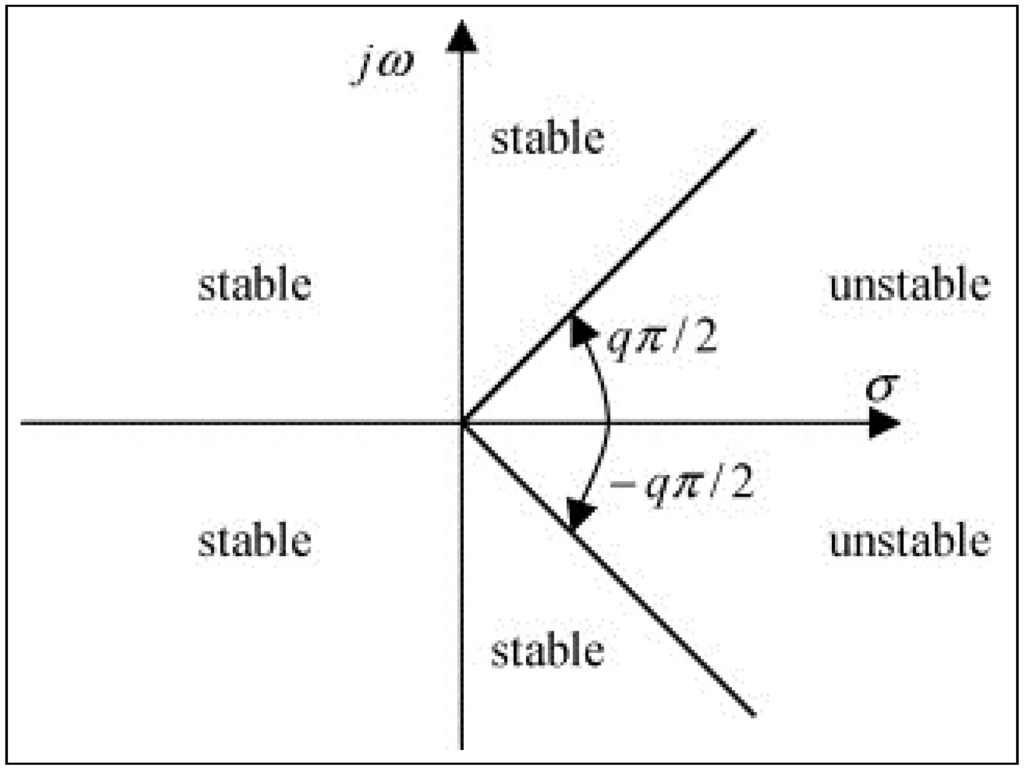
Figure 1. Stability region of the fractional order system (3).

Figure 1. Stability region of the fractional order system (3).

2.3. The Adams–Bashforth–Moulton Algorithm

We recall here the improved version of Adams–Bashforth–Moulton algorithm [17] for the fractional-order systems. Consider the fractional order initial value problem:

$$\left\{{\displaystyle \begin{array}{c}{\displaystyle D_t^{\alpha }x=f\left(x\left(t\right)\right)0\le t\le T,}\hfill \\ {\displaystyle x^{\left(k\right)}\left(0\right)=x_0^{\left(k\right)},k=0,1,...,m-1.}\hfill \end{array}}\right.$$

(5)

It is equivalent to the Volterra integral equation:

$${\displaystyle x\left(t\right)=\sum _{k=0}^{\left[\alpha \right]-1}{x}_0^{\left(k\right)}\frac{t^k}{k!}+\frac{1}{\Gamma \left(\alpha \right)}{\int }_0^t{(t-s)}^{\alpha -1}f(s,x\left(s\right))ds.}$$

(6)

Diethelm et al. have given a predictor-corrector scheme (see [17]), based on the Adams–Bashforth–Moulton algorithm, to integrate Equation (6). By applying this scheme to the fractional order system (5), and setting:

$${\displaystyle h=\frac{T}{N},t_n=nh,n=0,1,...,N,}$$

Equation (6) can be discretized as follows:

$$x_h\left(t_{n+1}\right)=\sum _{k=0}^{\left[\alpha \right]-1}{x}_0^{\left(k\right)}\frac{t^k}{k!}+\frac{h^{\alpha }}{\Gamma (\alpha +2)}f(t_{n+1},x_h^p\left(t_{n+1}\right))+\frac{h^{\alpha }}{\Gamma (\alpha +2)}\sum _{j=0}^n{a}_{j,n+1}f(t_j,x_h\left(t_j\right)),$$

(7)

where:

$$a_{j,n+1}=\left\{\begin{array}{cc}{\displaystyle n^{\alpha +1}-(n-\alpha ){(n+1)}^{\alpha },}& j=0,\hfill \\ {\displaystyle {(n-j+2)}^{\alpha +1}+{(n-j)}^{\alpha +1}-2{(n-j+1)}^{\alpha +1},}& 1\le j\le n,\hfill \\ {\displaystyle 1,}& j=n+1,\hfill \end{array}\right.$$

(8)

and the predictor is given by:

$${\displaystyle x_h^p\left(t_{n+1}\right)=\sum _{k=0}^{\left[\alpha \right]-1}{x}_0^{\left(k\right)}\frac{t^k}{k!}+\frac{1}{\Gamma \left(\alpha \right)}\sum _{j=0}^n{b}_{j,n+1}f(t_j,x_h\left(t_j\right)),}$$

(9)

where ${\displaystyle b_{j,n+1}=\frac{h^{\alpha }}{\alpha }{((n+1)-j)}^{\alpha }-{(n-j)}^{\alpha }.}$ The error estimate of the above scheme is:

$${\displaystyle {max}_{j=0,1,..,N}\left\{|x\left(t_j\right)-x_h\left(t_j\right)|\right\}=O\left(h^p\right),}$$

in which $p=min(2,1+\alpha )$.

3. A Fractional Order Economic System

We consider a 3D system of fractional order autonomous differential equations; this system can be interpreted as an idealized macroeconomic model with foreign capital investments [18]. It can be described by:

$$\left\{\begin{array}{c}{D}^{\alpha }x=my+px(d-y^2),\hfill \\ D^{\alpha }y=-x+cz,\hfill \\ D^{\alpha }z=sx-ry.\hfill \end{array}\right.$$

(10)

where $\alpha \in (0,1]$ and the state variables, x, y and z, are the savings of households, the gross domestic product (GDP) and the foreign capital inflow, respectively. Furthermore, the fractional derivation is considered with respect to time. Positive parameters represent corresponding ratios: m is the marginal propensity to saving, p is the ratio of capitalized profit, d is the value of the potential GDP, c is the output/capital ratio, s is the capital inflow/savings ratio and r is the debt refund/output ratio.

3.1. Dynamical Behavior

When $m=0.02$, $p=0.4$, $c=50$, $d=1$, $r=0.1$ and $s=10.$ The system (10) has three real equilibria $E_0(0,0,0)$, $E_1(0.024,2.4,4.8\times {10}^{-4})$ and $E_2(-0.024,-2.4,-4.8\times {10}^{-4})$.

At the equilibrium point $E_0$, the Jacobian matrix of System (10) is given by:

$${\displaystyle J{|}_{E_0}=\left(\begin{array}{ccc}pd& m& 0\\ -1& 0& c\\ s& -r& 0\end{array}\right),}$$

The eigenvalues of above matrix are given by:

$$\begin{array}{c}\hfill {\lambda }_1=1.6761839,{\lambda }_2=-0.6380920+2.5984529iand{\lambda }_3=-0.6380920-2.5984529i.\end{array}$$

Hence, the equilibrium point $E_0$ is unstable. At the equilibrium point $E_1$ and $E_2$, the Jacobian matrix of System (10) is given by:

$${\displaystyle J{|}_{E_{1,2}}=\left(\begin{array}{ccc}pd-5.76p& m-0.115p& 0\\ -1& 0& c\\ s& -r& 0\end{array}\right),}$$

The eigenvalues of the above matrix are given by:

$$\begin{array}{c}\hfill {\lambda }_1=-2.8852598,{\lambda }_2=0.4906299+2.7503585iand{\lambda }_3=0.4906299-2.7503585i.\end{array}$$

Here, ${\lambda }_1$ is a negative real number and ${\lambda }_2$ and ${\lambda }_3$ are a pair of complex conjugate eigenvalues with positive real parts. Therefore, the equilibrium points $E_1$ and $E_2$ are unstable. According to Theorem (4), System (10) exhibits chaotic behavior for $\alpha \ge {\alpha }_{min}=0.8876170531.$ We stress here that the case $\alpha =1$ was studied in [18].

3.2. Numerical Simulations

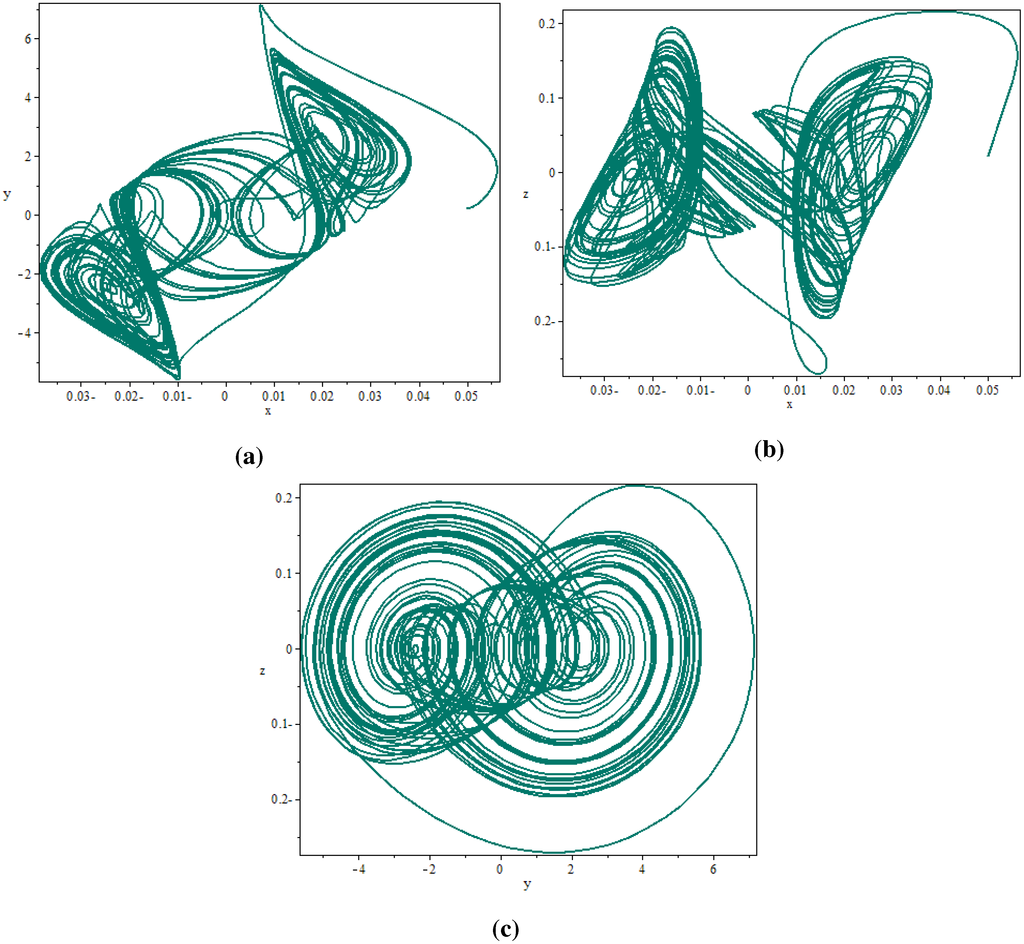
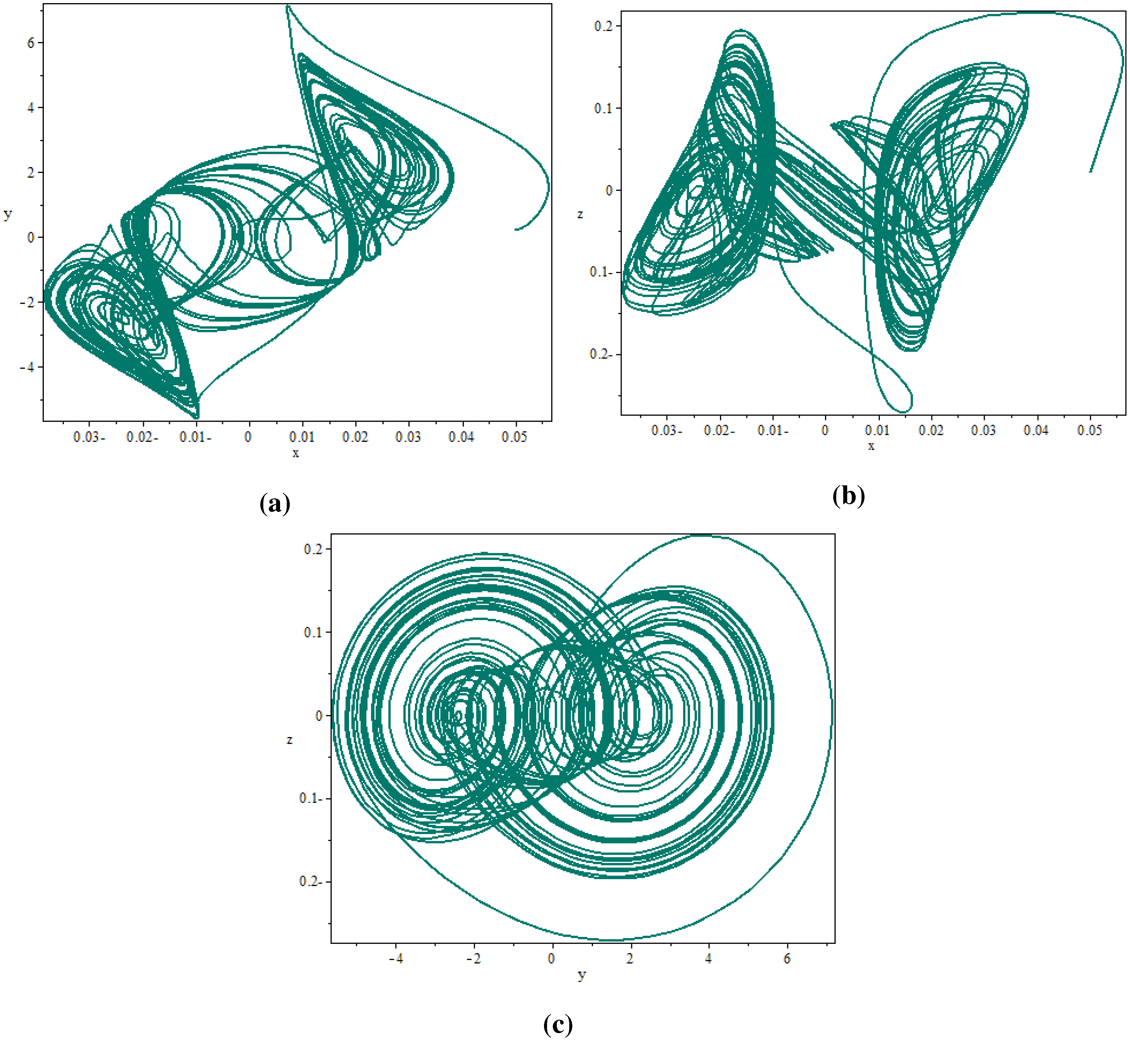
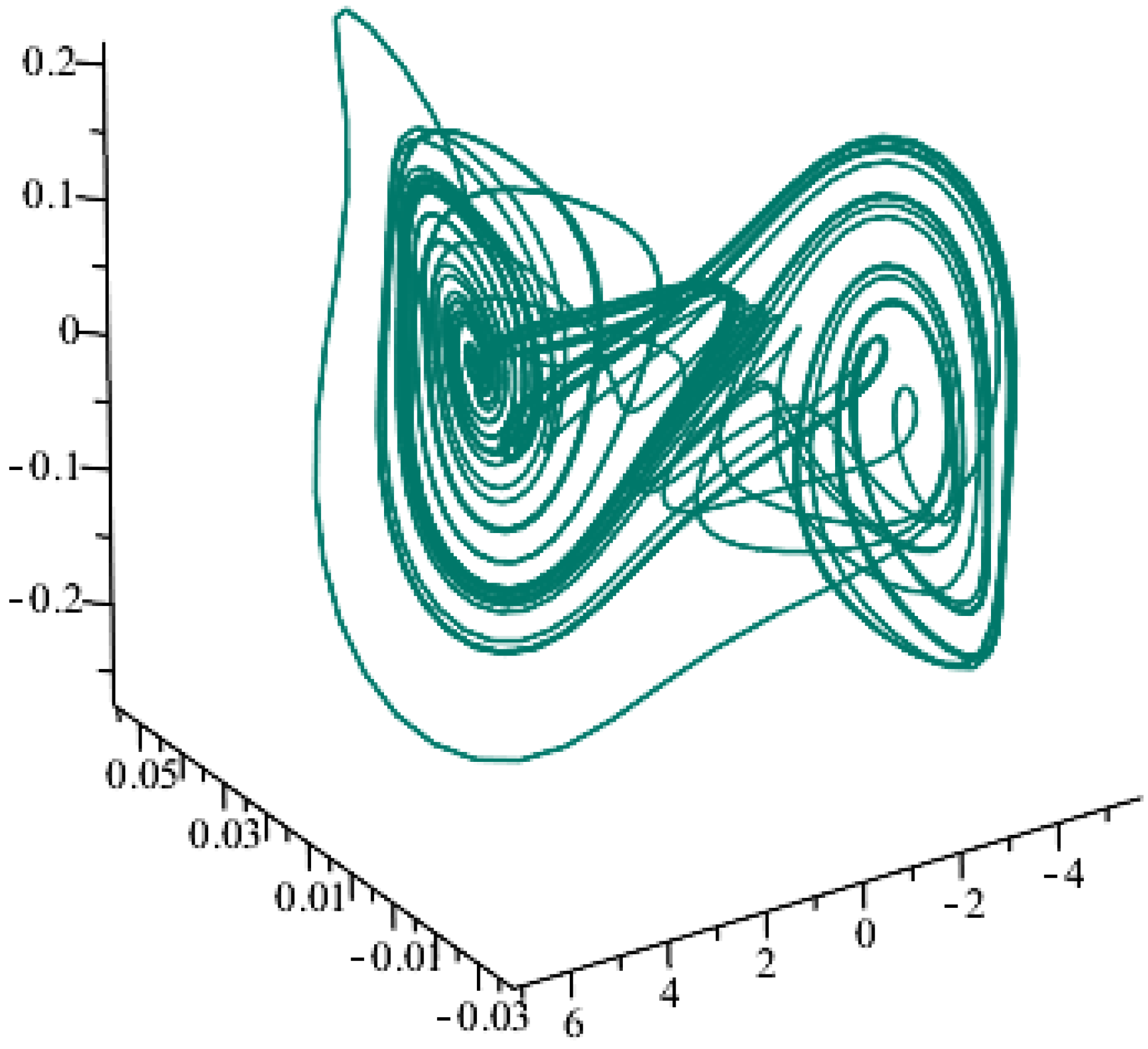
In order to confirm the chaotic behavior of System (10), numerical simulations were conducted for $\alpha =0.9$ and the selected initial conditions $(x_0,y_0,z_0)=(0.05,0.1,0.02).$ The time histories of the state variables, x, y and z, are graphically presented in Figure 2, and the phase diagrams are shown is Figure 3, while the chaotic attractor is plotted in Figure 4.

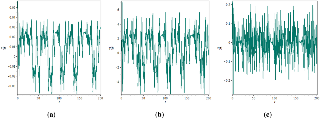
Figure 2. The time histories of variables (a) x(t), (b) y(t) and (c) z(t) for α = 0.9.

Figure 2. The time histories of variables (a) x(t), (b) y(t) and (c) z(t) for α = 0.9.

Figure 3. Phase portraits: (a) x − y, (b) x − z and (c) y − z for System (10) when α = 0.9.

Figure 3. Phase portraits: (a) x − y, (b) x − z and (c) y − z for System (10) when α = 0.9.

Figure 4. Chaotic attractor xyz for System (10) when α = 0.9.

Figure 4. Chaotic attractor xyz for System (10) when α = 0.9.

4. Active Control of the Fractional Order Chaotic System

In this section, we investigate the problem of chaos control of the fractional chaotic System (10). In order to control it towards equilibrium points $E_0$, $E_1$ and $E_2$, as in [19], we assume that the controlled fractional order autonomous system is given by:

$$\left\{\begin{array}{c}{D}^{\alpha }x=my+px(d-y^2)+U_1,\hfill \\ D^{\alpha }y=-x+cz+U_2,\hfill \\ D^{\alpha }z=sx-ry+U_3.\hfill \end{array}\right.$$

(11)

where $U_j\left(t\right)$ ($j=1,2,3$) are external active control inputs, which will be suitably-determined later. We prove the following result:

Theorem 2. Starting from any initial condition, an equilibrium point $E_i$ of system (11) is asymptotically stable when the controller $U_j$, $j=1,2,3$, is active, for $\alpha \ge {\alpha }_{min}$.

Proof. As a Lyapunov candidate function associated with System (11), we consider the quadratic function defined by:

$${\displaystyle V(t,(X\left(t\right)-E_i))={(x-x_i)}^2+{(y-y_i)}^2+{(z-z_i)}^2,}$$

(12)

where $X={(x,y,z)}^T$ and $E_i={(x_i,y_i,z_i)}^T$ is an equilibrium point. Note that V is a positive-definite function on ${\mathbb{R}}^3$. From system (11), we have:

$${\displaystyle D^{\alpha }V(t,(X\left(t\right)-E_i))=-2V(t,(X\left(t\right)-E_i))<0.}$$

(13)

According to the Lyapunov theory, the equilibrium point $E_i$ is asymptotically stable.

To stabilize the chaotic orbits in (10) to its equilibrium $E_0$ (respectively, $E_1$ or $E_2$), we need to add the following active controllers:

• For $E_0$:

  $$\left\{\begin{array}{c}U1:=-1.4x+0.98y+0.4x{y}^2,\hfill \\ U2:=-y-49.9z,\hfill \\ U3:=-10x-z.\hfill \end{array}\right.$$

  (14)
• For $E_1$:

  $$\left\{\begin{array}{c}{U}_1=0.904x+1.02608y-0.002304+0.4x{y}^2+1.92xy+0.0096y^2,\hfill \\ U_2=-y-49.9z,\hfill \\ U_3=-10x-z.\hfill \end{array}\right.$$

  (15)
• For $E_2$:

  $$\left\{\begin{array}{c}{U}_1=0.904x+1.02608y+0.002304+0.4x{y}^2-1.92xy-0.0096y^2,\hfill \\ U_2=-y-49.9z,\hfill \\ U_3=-10x-z.\hfill \end{array}\right.$$

  (16)

Taking into account the above-described controllers, the equilibria $E_0$, $E_1$ and $E_2$ are stabilized, and then, the chaos is controlled in system (10).

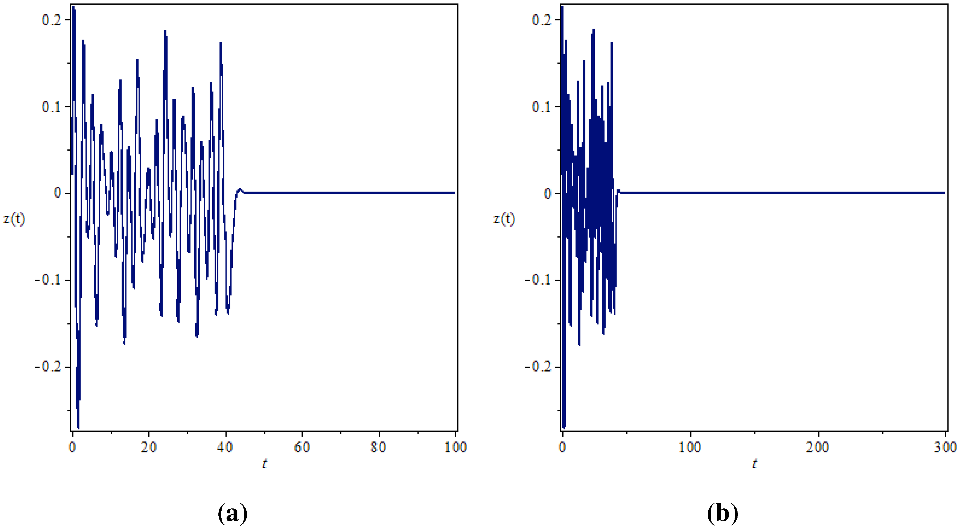
Now, we implement the improved Adams–Bashforth algorithm for numerical simulations (for $t\in [0,100]$ and $t\in [0,300]$). The unstable point $E_0$ has been stabilized, as shown in Figure 5, Figure 6 and Figure 7. We remark that the behaviors of $x\left(t\right),y\left(t\right)$ and $z\left(t\right)$ start as chaotic; then, when the control is activated at $t=40$, the equilibrium point is rapidly stabilized. The equilibria $E_1$ and $E_2$ are stabilized in an analogous way (see Figure 8, Figure 9, Figure 10, Figure 11, Figure 12 and Figure 13).

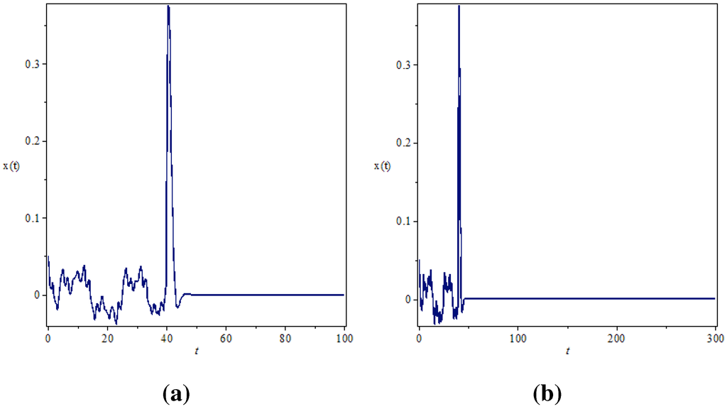
Figure 5. Time histories of System (11) for x signal at the equilibrium E₀ with α = 0.9: (a) t_max = 100, (b) t_max = 300.

Figure 5. Time histories of System (11) for x signal at the equilibrium E₀ with α = 0.9: (a) t_max = 100, (b) t_max = 300.

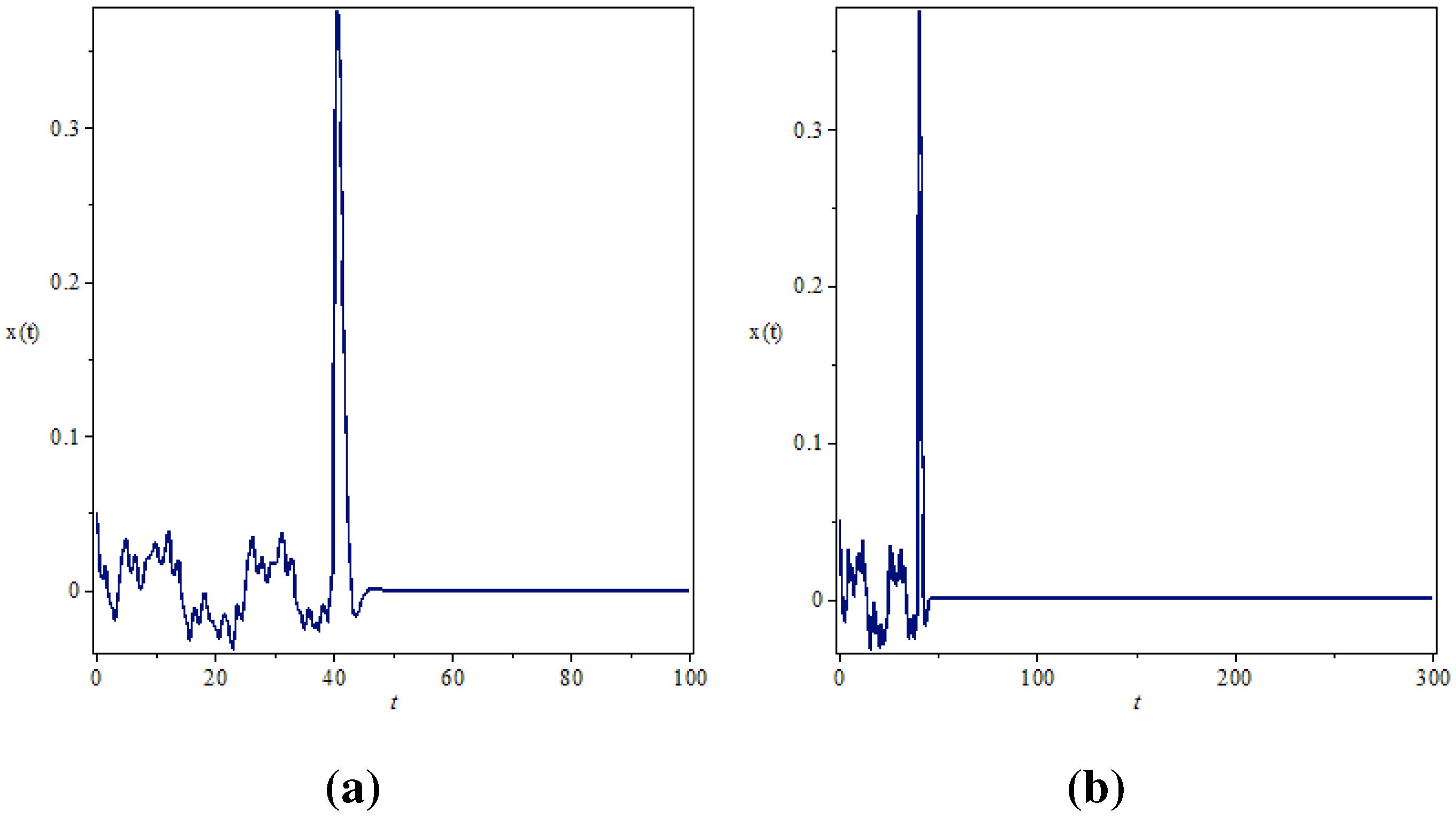
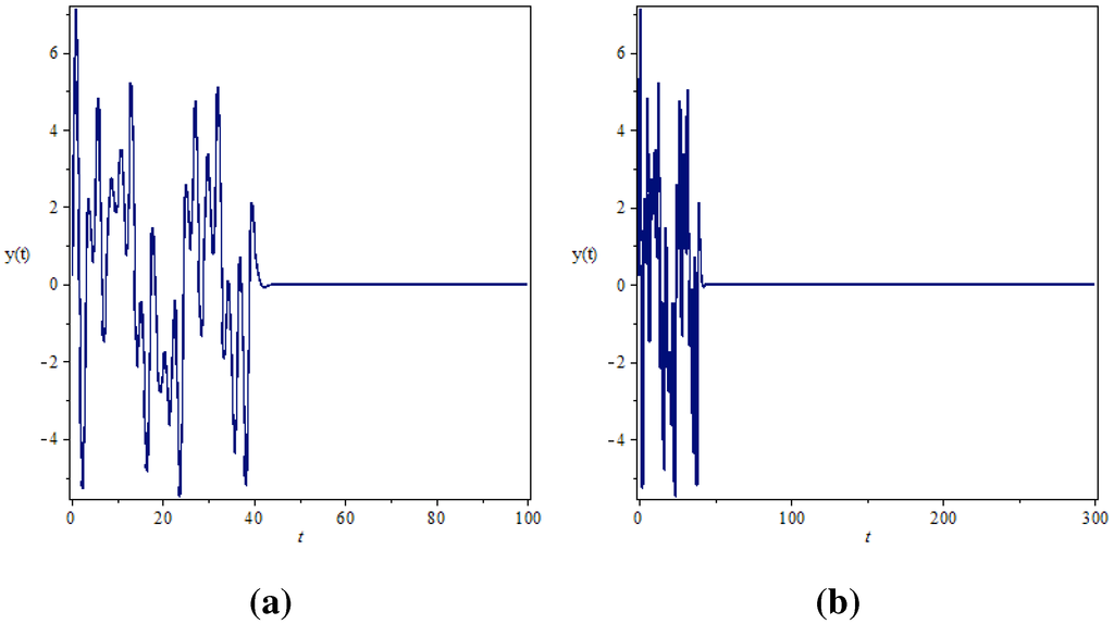
Figure 6. Time histories of system (11) for y signal at the equilibrium E₀ with α = 0.9: (a) t_max = 100, (b) t_max = 300.

Figure 6. Time histories of system (11) for y signal at the equilibrium E₀ with α = 0.9: (a) t_max = 100, (b) t_max = 300.

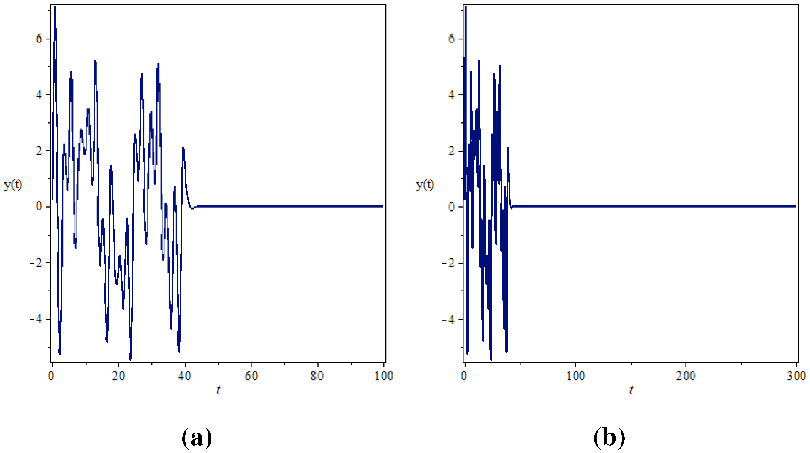
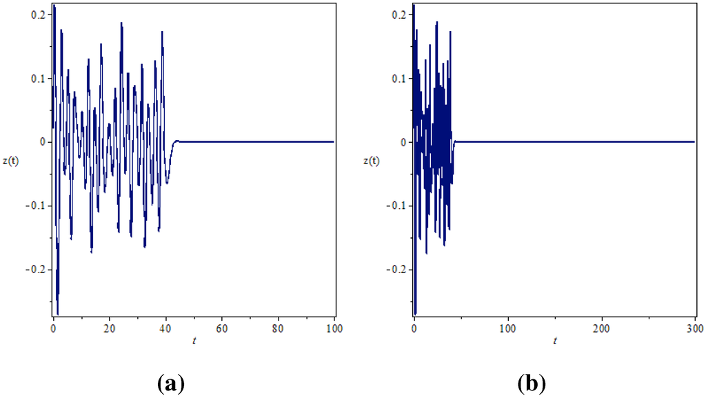
Figure 7. Time histories of System (11) for z signal at the equilibrium E₀ with α = 0.9: (a) t_max = 100, (b) t_max = 300.

Figure 7. Time histories of System (11) for z signal at the equilibrium E₀ with α = 0.9: (a) t_max = 100, (b) t_max = 300.

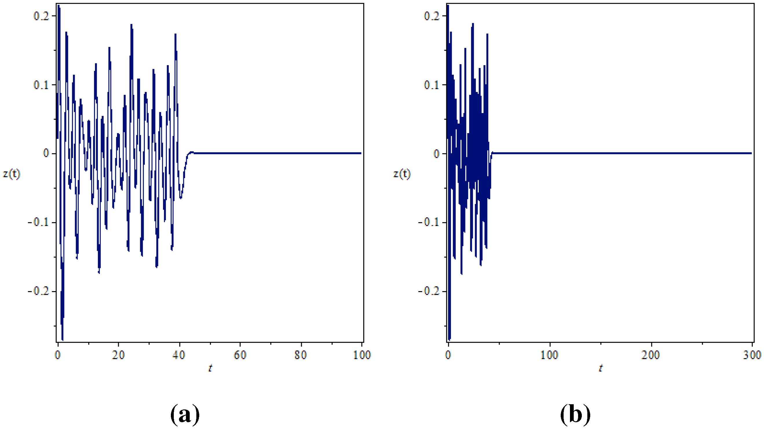
Figure 8. Time histories of System (11) for x signal at the equilibrium E₁ with α = 0.9: (a) t_max = 100, (b) t_max = 300.

Figure 8. Time histories of System (11) for x signal at the equilibrium E₁ with α = 0.9: (a) t_max = 100, (b) t_max = 300.

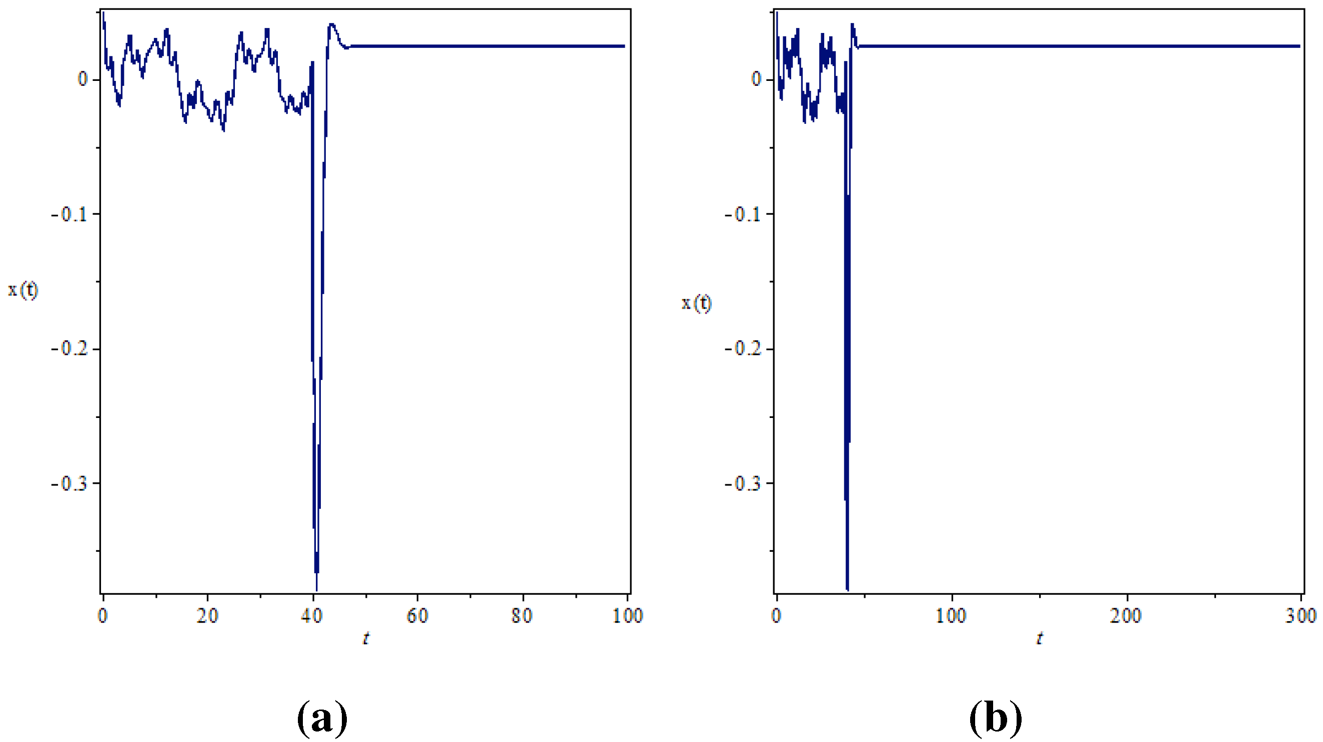
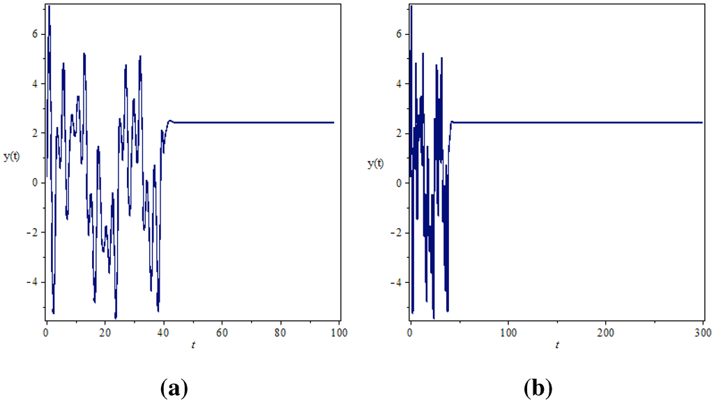
Figure 9. Time histories of System (11) for y signal at the equilibrium E₁ with α = 0.9: (a) t_max = 100, (b) t_max = 300.

Figure 9. Time histories of System (11) for y signal at the equilibrium E₁ with α = 0.9: (a) t_max = 100, (b) t_max = 300.

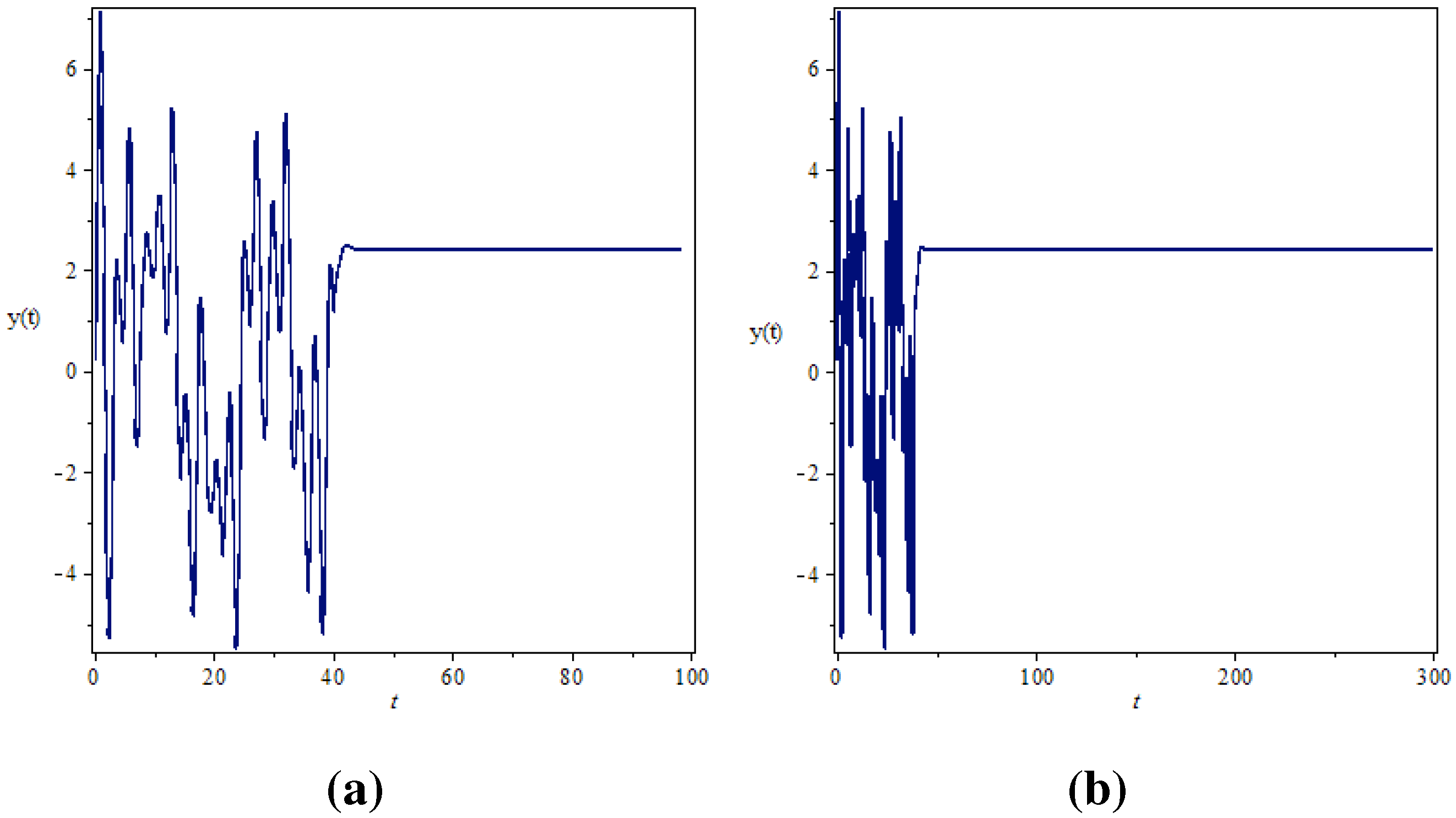
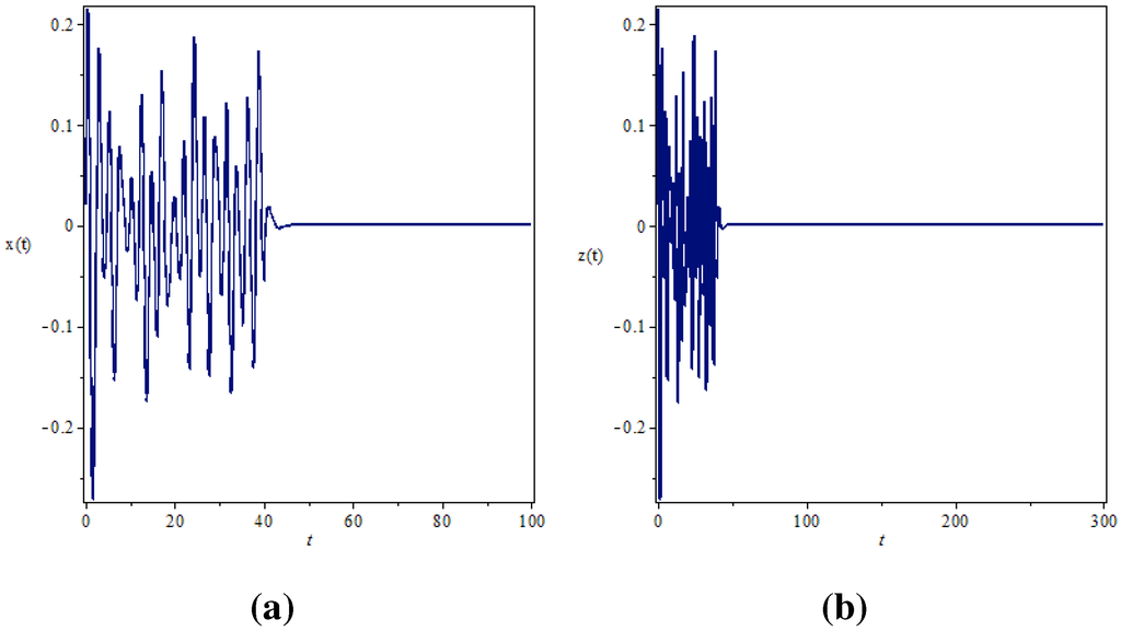
Figure 10. Time histories of System (11) for z signal at the equilibrium E₁ with α = 0.9: (a) t_max = 100, (b) t_max = 300.

Figure 10. Time histories of System (11) for z signal at the equilibrium E₁ with α = 0.9: (a) t_max = 100, (b) t_max = 300.

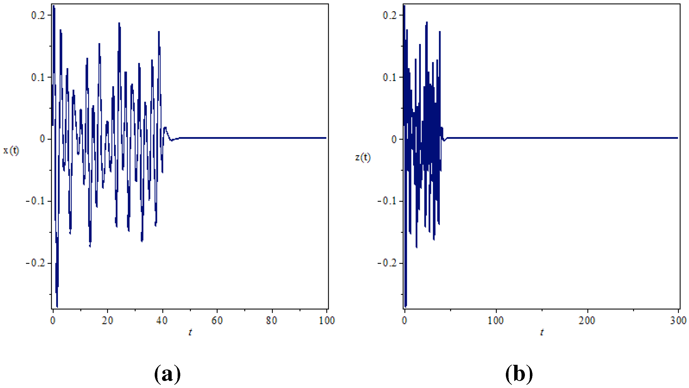
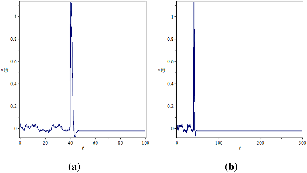
Figure 11. Time histories of System (11) for x signal at the equilibrium E₂ with α = 0.9: (a) t_max = 100, (b) t_max = 300.

Figure 11. Time histories of System (11) for x signal at the equilibrium E₂ with α = 0.9: (a) t_max = 100, (b) t_max = 300.

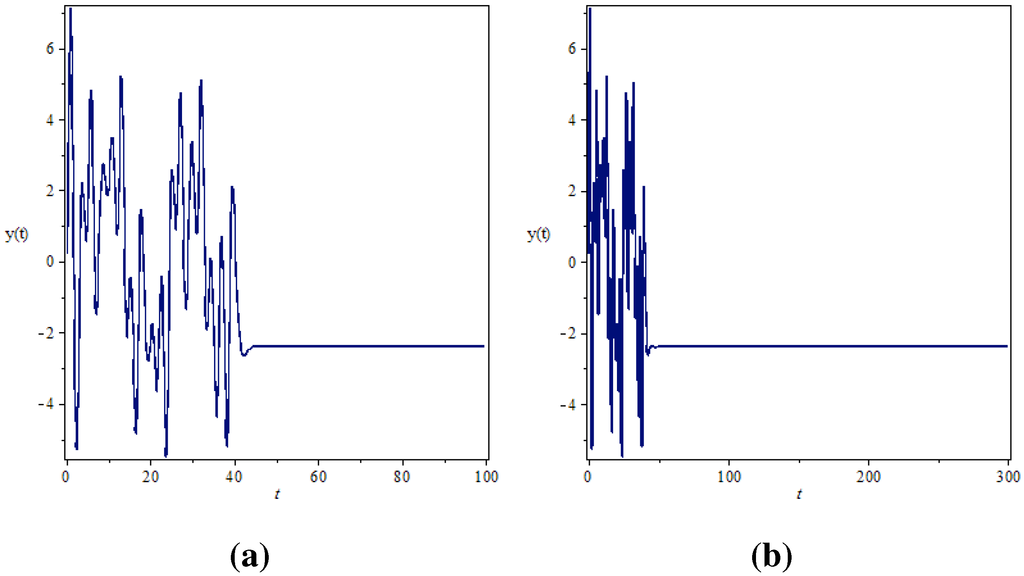
Figure 12. Time histories of System (11) for y signal at the equilibrium E₂ with α = 0.9: (a) t_max = 100, (b) t_max = 300.

Figure 12. Time histories of System (11) for y signal at the equilibrium E₂ with α = 0.9: (a) t_max = 100, (b) t_max = 300.

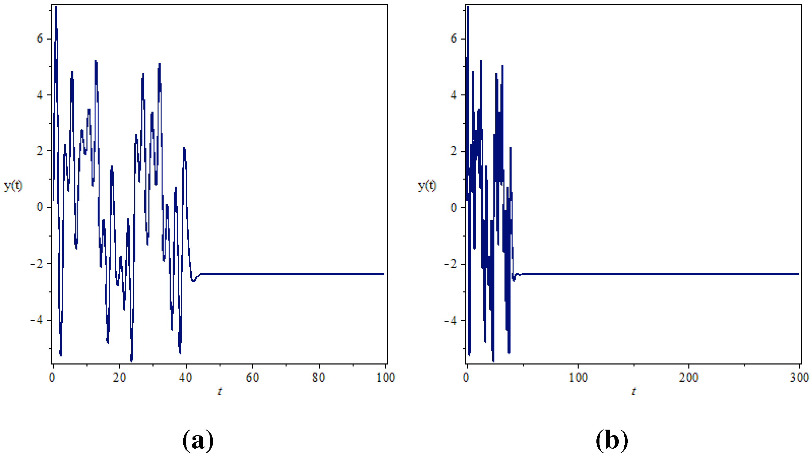
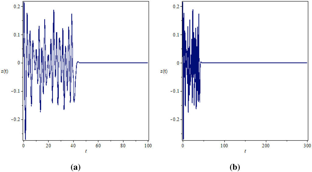
Figure 13. Time histories of System (11) for z signal at the equilibrium E₂ with α = 0.9: (a) t_max = 100, (b) t_max = 300.

Figure 13. Time histories of System (11) for z signal at the equilibrium E₂ with α = 0.9: (a) t_max = 100, (b) t_max = 300.

5. Conclusion

In this paper, chaos control of a fractional-order chaotic economic system is studied. Furthermore, we have studied the local stability of the equilibria using the Matignon stability condition. Analytical conditions for nonlinear active control have been implemented. Simulation results have illustrated the effectiveness of the proposed control method.

References

- Belgacem, F.B.M.; Baskonus, H.M.; Bulut, H. Variational Iteration Method for Hyperchaotic Nonlinear Fractional Differential Equations Systems. In Advances in Mathematics and Statistical Sciences, Proceedings of the 3rd International Conference on Mathematical, Computational and Statistical Sciences, (MCSS’15), Dubai, United Arab Emirates, 22–24 February 2015; pp. 445–453.
- Miller, K.S.; Rosso, B. An Introduction to the Fractional Calculus and Fractional Differential Equations; Wiley: New York, NY, USA, 1993. [Google Scholar]
- Oldham, K.B.; Spanier, J. The Fractional Calculus; Academic Press: New York, NY, USA, 1974. [Google Scholar]
- Nagy, A.M.; Sweilam, N.H. An efficient method for solving fractional Hodgkin–Huxley model. Phys. Lett. A 2014, 378, 1980–1984. [Google Scholar] [CrossRef]
- Sweilam, N.H.; Nagy, A.M.; El-Sayed, A.A. Second kind shifted Chebyshev polynomials for solving space fractional order diffusion equation. Chaos Solitons Fractals 2015, 73, 141–147. [Google Scholar] [CrossRef]
- Petras, I. Fractional-Order Nonlinear Systems: Modeling, Analysis and Simulation; Springer: Berlin/Heidelberg, Germany, 2011. [Google Scholar]
- Baleanu, D.; Guvenc, B.; Tenreiro-Machado, J.A. New Trends in Nanotechnology and Fractional Calculus Applications; Springer: New York, NY, USA, 2010. [Google Scholar]
- Bulut, H.; Belgacem, F.B.M.; Baskonus, H.M. Some New Analytical Solutions for the Nonlinear Time-Fractional KdV-Burgers-Kuramoto Equation. In Advances in Mathematics and Statistical Sciences, Proceedings of the 3rd International Conference on Mathematical, Computational and Statistical Sciences, (MCSS’15), Dubai, United Arab Emirates, 22–24 February 2015; pp. 118–129.
- Caponetto, R.; Dongola, G.; Fortuna, L. Fractional Order Systems: Modeling and Control Application; World Scientific: Singapore, Singapore, 2010. [Google Scholar]
- Caponetto, R.; Fazzino, S. An application of Adomian Decomposition Method for analysis of fractional-order chaotic systems. Int. J. Bifurc. Chaos 2013, 23, 1–7. [Google Scholar] [CrossRef]
- Tavazoei, M.; Haeri, M. A necessary condition for double scroll attractor existence in fractional-order systems. Phys. Lett. A 2007, 367, 102–113. [Google Scholar] [CrossRef]
- Wang, S.; Yu, Y. Application of Multistage Homotopy-perturbation Method for the Solutions of theChaotic Fractional Order Systems. Int. J. Nonlinear Sci. 2012, 13, 3–14. [Google Scholar]
- Zaslavsky, G. Hamiltonian Chaos and Fractional Dynamics; Oxford University Press: Oxford, UK, 2008. [Google Scholar]
- Podlubny, I. Fractional Differential Equations: Mathematics in Science and Engineering; Academic Press: Waltham, MA, USA, 1999. [Google Scholar]
- Caputo, M. Linear models of dissipation whose Q is almost frequency independent. J. R. Astral. Soc. 1967, 13, 529–539. [Google Scholar] [CrossRef]
- Matignon, D. Stability results for fractional differential equations with applications to control processing. In Proceedings of IMACS Multiconference on Computational Engineering in Systems Applications, Lille, France, 9–12 July 1996; pp. 963–968.
- Diethelm, K.; Ford, N.; Freed, A.; Luchko, A. Algorithms for the fractional calculus: A selection of numerical method. Comput. Methods Appl. Mech. Eng. 2005, 94, 743–773. [Google Scholar] [CrossRef]
- Volos, C.K.; Ioannis, M.K.; Ioannis, N.S. Synchronization Phenomena in Coupled Nonlinear Systems Applied in Economic Cycles. WSEAS Trans. Syst. 2012, 11, 681–690. [Google Scholar]
- Hammouch, Z.; Mekkaoui, T. Control of a new chaotic fractional-order system using Mittag-Leffler stability. Nonlinear Stud. 2015. to appear. [Google Scholar]
© 2015 by the authors; licensee MDPI, Basel, Switzerland. This article is an open access article distributed under the terms and conditions of the Creative Commons Attribution license (http://creativecommons.org/licenses/by/4.0/).