Preference Inconsistence-Based Entropy

Abstract

Preference analysis is a class of important issues in ordinal decision making. As available information is usually obtained from different evaluation criteria or experts, the derived preference decisions may be inconsistent and uncertain. Shannon entropy is a suitable measurement of uncertainty. This work proposes the concepts of preference inconsistence set and preference inconsistence degree. Then preference inconsistence entropy is introduced by combining preference inconsistence degree and Shannon entropy. A number of properties and theorems as well as two applications are discussed. Feature selection is used for attribute reduction and sample condensation aims to obtain a consistent preference system. Forward feature selection algorithm, backward feature selection algorithm and sample condensation algorithm are developed. The experimental results show that the proposed model represents an effective solution for preference analysis.

1. Introduction

Multiple attribute decision making refers to making preference decisions between available alternatives characterized by multiple, usually conflicting, attributes [1]. A multiple attributes decision making system can be depicted by using the alternative performance matrix, where element $x_{ij}$ is the rating of alternative i with respect to attribute j. A weight vector is designed to indicate the significance of every attribute. Various methods for finding weights can be found in the literature, such as the analytic hierarchy process (AHP) method [2], weighted least squares method [3], Delphi method [4], the entropy method, multiple objective programming [5,6], principal element analysis [6], etc. Ordinal decision making is a class of important issues in multiple attribute decision making where the conditional attributes and the decision are all ordinal. There are numerous applications associated with an assignment of objects evaluated by a set of criteria to pre-defined preference-ordinal decision classes, such as credit approval, stock risk estimation, and teaching evaluations [7]. The alternative performance matrix and weights vector method cannot reflect the ordinal nature of decisions based on conditional attributes, therefore, is not a suitable tool for ordinal decision making.

Preference analysis is a class of important issues in ordinal decision making. Preference relations are very useful in expressing a decision maker’s preference information in decision problems in various fields. During the past years, the use of preference relations has received increasing attention, and a number of studies have focused on this issue, and various types of preference relations have been developed, such as, multiplicative preference relation introduced by Saaty [2], incomplete multiplicative preference relation introduced by Harker [8], interval multiplicative preference relation introduced by Saaty and Vargas [9], incomplete interval multiplicative preference relation introduced by Xu [10], triangular fuzzy multiplicative preference relation introduced by Van Laarhoven and Pedrycz [11], fuzzy preference relation introduced by Luce and Suppes [12], incomplete fuzzy preference relation introduced by Alonso et al. [13], interval fuzzy preference relation introduced by Xu and Herrera et al., and linguistic preference relation introduced by Herrera et al. [14,15,16].

One task of preference analysis is to predict a decision maker’s preference according to available information. A lot of methods for preference analysis can be found in the literature. Greco et al. introduced a dominance rough set model that is suitable for preference analysis [17,18]. They extracted dominance relations from multiple criteria, and constructed similarity relations and equivalence relations from numerical attributes and nominal features respectively. In [19], Hu et al. developed a rough set model based on fuzzy preference by integrating fuzzy preference relations with fuzzy rough set model, and generalized the dependency to compute relevance between the criteria and decision and obtain attribute reductions. In ordinal decision making, there exists a basic assumption that better conditions should result in better decisions, which usually holds for a single criterion. For multi-criteria ordinal decision system, however, the decision is made considering various sources of information which is usually obtained from different evaluation criteria or experts and thus the decision preference might be inconsistent with some criteria.

Preference inconsistence leads to decision uncertainty. One of the decision uncertainty measures which have been proposed by researchers is the Shannon entropy concept. The entropy concept is used in various scientific fields. In transportation models, entropy acts as a measure of dispersal of trips between origin and destinations. In physics, the word entropy has important physical implications as the amount of “disorder” of a system. Also the entropy associated with an event is a measure of the degree of randomness in the event. The concept of Shannon’s entropy has an important role in information theory and is used to refer to a general measure of uncertainty [1]. In preference analysis, some methods based on entropy have been introduced in the literature. Abbas presented an optimal question-selection algorithm to elicit von Neumann and Morgenstern utility values by using information theory and entropy-coding principles for a set of ordered prospects of a decision situation [20]. Lotfi extended the Shannon entropy method to interval data for obtaining the weights of criteria of a multiple attributes decision making problem [1]. Yang and Qiu proposed the expected utility-entropy (EU-E) measure of risk and a decision making model about preference orderings among gambles based on expected utility and entropy of an action involving risk [21]. Abbas introduced an analogy between probability and utility through the notion of a utility density function and illustrate the application of this analogy to the maximum entropy principle [22]. A normative method was presented to assign unbiased utility values when only incomplete preference information was available about the decision maker [23]. In this research, Shannon entropy has been expanded to preference inconsistence entropy and then is used to measure the uncertainty of preference decision to conditional attributes.

Based on this idea, the contributions of this work include: (1) this paper defines a preference inconsistence set and preference inconsistence degree, and some properties are given; (2) based on preference inconsistence degree and Shannon entropy, the notion of preference inconsistence entropy is proposed; (3) relative attribute significance is defined, feature selection is investigated, and meanwhile, a forward feature selection algorithm and backward feature selection algorithm are developed; (4) a sample condensation algorithm is also given; (5) finally, some experiments are completed to verify the proposed approach. The experimental results show that relative attribute significance based on preference inconsistence entropy can reflect the significance of features in a preference decision and the developed feature selection and sample condensation algorithms are helpful to make the data set preference consistent.

The remainder of the paper is organized as follows: Section 2 provides a brief overview of preference relations and Shannon entropy, and some basic formulas that will be used in the remaining sections of this paper are given. In Section 3, the concepts of preference inconsistence degree and preference inconsistence entropy (PIE) are proposed. Some properties of PIE are discussed and a series of theorems are put forward. Section 4 presents two applications of PIE: feature selection and sample condensation. Relative attribute significance is defined. A forward feature selection algorithm and backward feature selection algorithm as well as sample condensation algorithm are developed. Numerical experiments are reported in Section 5. Finally, Section 6 wraps up with conclusions.

2. Preliminary Knowledge

In this section, we will review some basic concepts about preference relation and information entropy, which have been addressed in [24,25,26,27,28,29,30,31].

2.1. Information Entropy

In 1948, Claude Shannon introduced the entropy term, nowadays named Shannon entropy. Shannon entropy is a simple quantitative measure of uncertainty. The following concepts are taken from Shannon’s original paper [30]. Let X be a random variable, taking a finite number of possible values $x_1,x_2, x_3, \dots , x_n$ with respective probabilities $p_i\ge 0$ for i = 1, 2, …, n and ${\sum }_{i=1}^n{p}_i=1$. The Shannon entropy H(X) is defined as:

$$H\left(X\right)=-{{\displaystyle \sum }}_{i=1}^n{p}_{i}log{p}_i$$

(1)

Suppose there are two events, X and Y, in question with m possibilities for the first and n for the second. Let p(i, j) be the probability of the joint occurrence of i for the first and j for the second. The entropy of the joint event is:

$$H\left(X,Y\right)=-{{\displaystyle \sum }}_{i,j}p\left(i,j\right)logp\left(i,j\right)$$

(2)

For any particular value i for X, we can assume there is a conditional probability $p\left(j|i\right)$ where Y has the value i. The conditional entropy of Y, $H\left(Y|X\right)$, is defined as the average of entropy of Y for each value of X weighted according to the probability of getting that particular X. That is:

$$\begin{array}{ll}H\left(Y|X\right)& =-{{\displaystyle \sum }}_{i,j}p\left(i,j\right)logp\left(j|i\right)\\ & =-{{\displaystyle \sum }}_{i,j}p\left(i,j\right)logp\left(i,j\right)+{{\displaystyle \sum }}_{i,j}p\left(i,j\right)log{\displaystyle \sum }_{j}p\left(i,j\right)\\ & =H\left(X,Y\right)-H\left(X\right)\end{array}$$

(3)

The conditional entropy of Y when X is known is the joint event X, Y minus the entropy of X. We will use this property to calculate the relative attribute significance for our feature selection algorithm.

2.2. Preference Relation

A decision system is a tuple $DS=<U,A\cup D,f>$, where U is a nonempty finite set of objects, $A=\left\{a_1,a_2,\dots ,a_m\right\}$ is a set of conditional attributes to characterize the objects, $D=\left\{d_1,d_2,\dots ,d_n\right\}$ is the decision, $f_a:U\to V_a$ is a mapping for any $a\in A$, where $V_a$ is called the value set of attribute a. The decision system DS is referred to as ordinal decision system, if $d_1\le d_2\le \dots \le d_n$, and $a_{i1}\le a_{i2}\le \dots \le a_{ik} \text{holds} \text{for any} a_i\in A$, where $\left\{a_{i1},a_{i2},\dots ,a_{ik}\right\}$ is the value set of conditional attribute $a_i\left(1\le i\le m\right)$.

Let $DS=<U,A\cup D,f>$ is an ordinal decision system. For preference analysis, the following relations are defined. $\forall C\subseteq A,x,y\in U$:

$$R_C^{\ge }=\left\{\left(x,y\right)\in U\times U :f\left(x,a\right)\ge f\left(y,a\right), \forall a\in C\right\}$$

(4)

$$R_C^{\le }=\left\{\left(x,y\right)\in U\times U :f\left(x,a\right)\le f\left(y,a\right), \forall a\in C\right\}$$

(5)

$$R_D^{\ge }=\left\{\left(x,y\right)\in U\times U :f\left(x,D\right)\ge f\left(y,D\right)\right\}$$

(6)

$$R_D^{\le }=\left\{\left(x,y\right)\in U\times U :f\left(x,D\right)\le f\left(y,D\right)\right\}$$

(7)

where $f\left(x,a\right)$ is attribute value of object x with respect to attribute a, and $f\left(x,D\right)$ is the decision of object x.

$R_C^{\ge }$ and $R_C^{\le }$ are referred to as conditional domination relation. $R_D^{\ge } \text{and} R_D^{\le }$ are referred to as decision domination relation.

If $\left(x,y\right)\in R_C^{\ge }$, we say that object x is greater than or equal to object y with respect to C. In other word, object x is not less than object y with respect to $C$.

If $\left(x,y\right)\in R_C^{\le }$, we say that object x is less than or equal to object y with respect to C. In other word, object x is not greater than object y with respect to $C$.

If $\left(x,y\right)\in R_D^{\ge }$, we say that the decision object x is better than or equal to object y. In other word, the decision of object x is not worse than that of y.

If $\left(x,y\right)\in R_D^{\le }$, we say that the decision object x is worse than or equal to object y. In other word, the decision of object x is not better than that of y.

In preference analysis, x’s decision should not be worse than y’s if x is better than y in terms of criterion a; otherwise, the decision is inconsistent [14]. Similarly, x’s decision should not be better than y’s if x is less than y in terms of criterion a; otherwise, the decision is inconsistent. $R^{\ge }$ and $R^{\le }$ stands only for relation of not less than and not greater than, respectively, but cannot represent relations strictly greater than and strictly less than. We extend the domination relation to strict preference relation:

$$R_C^{>}=\{\left(x,y\right)\in U\times U :f\left(x,a\right)>f\left(y,a\right), \forall a\in C\}$$

(8)

$$R_C^{<}=\{\left(x,y\right)\in U\times U :f\left(x,a\right)<f\left(y,a\right), \forall a\in C\}$$

(9)

$$R_D^{>}=\left\{\left(x,y\right)\in U\times U :f\left(x,D\right)>f\left(y,D\right)\right\}$$

(10)

$$R_D^{<}=\left\{\left(x,y\right)\in U\times U :f\left(x,D\right)<f\left(y,D\right)\right\}$$

(11)

If $\left(x,y\right)\in R_C^{>}$, we say object x is better than object y with respect to $C$. If $\left(x,y\right)\in R_C^{\le }$, we say object x is less than object x with respect to $C$.

If $\left(x,y\right)\in R_D^{>}$, we say the decision of object x is better than that of y. If $\left(x,y\right)\in R_D^{\le }$, we say the decision of object x is less than that of y.

In this work, $R^{\ge }$ and $R^{>}$ are all named as upward domination relations, and $R^{\le }$ and $R^{<}$ are all named as downward domination relations. The preference information granulation can be represented as:

$${\left[x\right]}_C^{\ge }=\left\{y\in U : \left(y,x\right)\in R_C^{\ge }\right\}$$

(12)

$${\left[x\right]}_C^{\le }=\left\{y\in U : \left(y,x\right)\in R_C^{\le }\right\}$$

(13)

$${\left[x\right]}_C^{>}=\left\{y\in U : \left(y,x\right)\in R_C^{>}\right\}$$

(14)

$${\left[x\right]}_C^{<}=\left\{y\in U : \left(y,x\right)\in R_C^{<}\right\}$$

(15)

Let $PS=<U,C\cup D,f>$ be an ordinal decision system, C is the set of conditional attributes and D is the decision, $D=\left\{d_1,d_2,\dots ,d_N\right\},d_1\le d_2\le \dots \le d_N$. $x\in U,a\in C$, if $\forall y\in {\left[x\right]}_a^{>}$, $f\left(y,D\right)\ge f\left(x,D\right)$ holds, we say object x is upward preference consistent in terms of attribute a. Otherwise, x is upward preference inconsistent in terms of a. Similarly, if $\forall y\in {\left[x\right]}_a^{<}$, $f\left(y,D\right)\le f\left(x,D\right)$ holds, we say object x is downward preference consistent in terms of attribute a, whereas, x is downward preference inconsistent in terms of a.

A lot of research has been done regarding preference consistent decision systems. In a real environment, however, we often need to face preference inconsistent cases. Preference inconsistence leads to preference analysis uncertainty. Those achievements for preference consistent system cannot be used to analyze preference inconsistent cases. Shannon entropy is a very good measure of uncertainty. Therefore, we will study the entropy based on preference inconsistence to deal with preference inconsistent issues.

3. Preference Inconsistence Based Entropy

In this section, two types of preference inconsistence entropy (PIE)—upward preference inconsistence entropy (UPIE) and downward preference inconsistence entropy (DPIE)—are introduced to measure the preference uncertainty. Some relative concepts and theorems will be discussed in detail.

Definition 1. 

Given a preference inconsistent ordinal decision system $PS=<U, C\cup D,f>.$ $\forall x\in U,a\in C$, the preference inconsistent set (PIS) of x in terms of a can be denoted by:

• upward preference inconsistent set (UPIS):

  $$uiconS\left(x,a\right)=\{y\in U|y\in {\left[x\right]}_a^{>} \bigwedge f\left(y,D\right)<f\left(x,D\right)\}$$

  (16)
• downward preference inconsistent set (DPIS):

  $$diconS\left(x,a\right)=\{y\in U|y\in {\left[x\right]}_a^{<} \bigwedge f\left(y,D\right)>f\left(x,D\right)\}$$

  (17)

For a set of attributes $\mathrm{B}\subseteq \mathrm{C}$, we have:

$$uiconS\left(x,B\right)=\{y\in U|y\in {\left[x\right]}_b^{>} \bigwedge f\left(y,D\right)<f\left(x,D\right),\forall b\in B\}$$

(18)

$$diconS\left(x,B\right)=\{y\in U|y\in {\left[x\right]}_b^{<} \bigwedge f\left(y,D\right)>f\left(x,D\right), \forall b\in B\}$$

(19)

For a set of attributes $B\subseteq C$, object x is upward preference consistent in terms of B if $\exists b\in B$, object x is upward preference consistent in terms of b, whereas, x is upward preference inconsistent in terms of B unless x is upward preference inconsistent in terms of each attribute in B. As to downward preference, a similar case occurs. If $\exists b\in B$, object x is downward preference consistent in terms of b, x is downward preference consistent in terms of B. Otherwise, x is downward preference inconsistent in terms of B.

Theorem 1. 

Let $PS=<U, C\cup D,f>$ be a preference inconsistent ordinal decision system, U is nonempty finite set of objects, C is the set of conditional attributes and D is the decision, $D=\left\{d_1,d_2,\dots ,d_N\right\}, d_1\le d_2\le \dots \le d_N$. Given two attributes $a_1,a_2\in C$, we have:

$$uiconS(x,a\cup b)=uiconS\left(x,a\right)\cap uiconS\left(x,b\right)$$

(20)

$$diconS(x,a\cup b)=diconS\left(x,a\right)\cap diconS\left(x,b\right)$$

(21)

Proof:

$$\begin{array}{ll}uiconS(x,a\cup b)& =\{y\in U|y\in {\left[x\right]}_a^{>} \bigwedge y\in {\left[x\right]}_b^{>} \bigwedge f\left(y,D\right)<f\left(x,D\right)\}\\ & =\{y\in U|y\in {\left[x\right]}_a^{>} \bigwedge y f\left(y,D\right)<f\left(x,D\right)\}\\ & \phantom{=}\cap \{y\in U|y\in {\left[x\right]}_b^{>} \bigwedge y f\left(y,D\right)<f\left(x,D\right)\}\\ & =uiconS\left(x,a\right)\cap uiconS\left(x,b\right)\end{array}$$

(22)

$$\begin{array}{ll}diconS(x,a\cup b)& =\{y\in U|y\in {\left[x\right]}_a^{<} \bigwedge y\in {\left[x\right]}_b^{<} \bigwedge f\left(y,D\right)>f\left(x,D\right)\}\\ & =\{y\in U|y\in {\left[x\right]}_a^{<} \bigwedge y f\left(y,D\right)>f\left(x,D\right)\}\\ & \phantom{=}\cap \{y\in U|y\in {\left[x\right]}_b^{<} \bigwedge y f\left(y,D\right)>f\left(x,D\right)\}\\ & =diconS\left(x,a\right)\cap diconS\left(x,b\right)\end{array}$$

(23)

☐

We can easily expand this theorem to a multiple attributes case:

$$uiconS\left(x,{{\displaystyle \cup }}_{i=1}^n{a}_i \right)={{\displaystyle \cap }}_{i=1}^{n}uiconS\left(x,a_i\right)$$

(24)

$$diconS\left(x,{{\displaystyle \cup }}_{i=1}^n{a}_i \right)={{\displaystyle \cap }}_{i=1}^{n}diconS\left(x,a_i\right)$$

(25)

Definition 2. 

Let $PS=<U,C\cup D,f>$ be a reference inconsistent ordinal decision system, C is the set of conditional attributes and D is the decision, $D=\left\{d_1,d_2,\dots ,d_N\right\},d_1\le d_2\le \dots \le d_N.$ Given $A\subseteq C$, the preference inconsistent degree (PID) can be defined as:

• upward preference inconsistent degree (UPID):

  $$upicd\left(x,A\right)=\frac{|uiconS\left(x,A\right)|}{|U|}$$

  (26)
• downward preference inconsistent degree (DPID):

  $$dpicd\left(x,A\right)=\frac{|diconS\left(x,A\right)|}{|U|}$$

  (27)

  where $uiconS \text{and} diconS$ are the set of upward and downward preference inconsistent set, respectively.

Theorem 2. 

Let $PS=<U, C\cup D,f>$ be a preference inconsistent ordinal decision system, U is a nonempty finite set of objects, C is the set of conditional attributes and D is the decision, $D=\left\{d_1,d_2,\dots ,d_N\right\}, d_1\le d_2\le \dots \le d_N$. Given two attributes $a_1,a_2\in C$, we have:

$$upicd\left(x,a_1\right)\ge uiconS(x,a_1\cup a_2)$$

(28)

$$upicd\left(x,a_2\right)\ge uiconS(x,a_1\cup a_2)$$

(29)

$$dpicd\left(x,a_1\right)\ge diconS(x,a_1\cup a_2)$$

(30)

$$dpicd\left(x,a_2\right)\ge diconS(x,a_1\cup a_2)$$

(31)

Proof. 

It can be proven easily by Definitions 2–4 and Theorem 1. □

The preference inconsistent information granule can be represented as follows:

$${\left[A\right]}^{\ge }=\frac{upicd\left(x_1,A\right)}{x_1} + \frac{upicd\left(x_2,A\right)}{x_2} + \frac{upicd\left(x_3,A\right)}{x_3} +\dots + \frac{upicd\left(x_4,A\right)}{x_4}$$

(32)

$${\left[A\right]}^{\le }=\frac{dpicd\left(x_1,A\right)}{x_1} + \frac{dpicd\left(x_2,A\right)}{x_2} + \frac{dpicd\left(x_3,A\right)}{x_3} +\dots + \frac{dpicd\left(x_4,A\right)}{x_n}$$

(33)

Definition 3. 

Let $PS=<U,C\cup D,f>$ be a preference inconsistent ordinal decision system, C is the set of conditional attributes and D is the decision, $D=\left\{d_1,d_2,\dots ,d_N\right\},d_1\le d_2\le \dots \le d_N$. The preference inconsistent entropy(PIE) can be defined as:

• upward preference inconsistent entropy (UPIE):

  $$UH\left(A\right)=-\frac{1}{|U|}{\displaystyle \sum }_{x_i\in U, upicd\left(x_i,A\right)\ne 0}{\log }_2\left(1-upicd\left(x_i,A\right)\right)$$

  (34)
• downward preference inconsistent entropy (DPIE):

  $$DH\left(A\right)=-\frac{1}{|U|}{\displaystyle \sum }_{x_i\in U,dpicd\left(x_i,A\right)\ne 0}{\log }_2\left(1-dpicd\left(x_i,A\right)\right)$$

  (35)

  where $upicd$ and $dpicd$ are the upward preference inconsistence degree and downward preference inconsistence degree, respectively. As for preference consistent ordinal decision system, the preference decisions are certain, and $UH\left(A\right)$ and $DH\left(A\right)$ are all equal to 0, which is consistent with Shannon entropy.

Definition 4. 

Let $PS=<U,C\cup D,f>$ be a preference inconsistent ordinal decision system, C is the set of conditional attributes and D is the decision, $D=\left\{d_1,d_2,\dots ,d_N\right\},d_1\le d_2\le \dots \le d_N$. Given two attributes $A_1,A_2\in C$, the preference inconsistent joint entropy (PIJE) is expressed as:

• upward preference inconsistent joint entropy (UPIJE):

  $$UH(A_1\cup A_2)=-\frac{1}{|U|}{\displaystyle \sum }_{x_i\in U,upicd\left(x_i,A_1\cup A_2\right)\ne 0}{\log }_2\left(1-upicd\left(x_i,A_1\cup A_2\right)\right)$$

  (36)
• downward preference inconsistent joint entropy (DPIJE):

  $$DH(A_1\cup A_2)=-\frac{1}{|U|}{\displaystyle \sum }_{x_i\in U,upicd\left(x_i,A_1\cup A_2\right)\ne 0}{\log }_2\left(1-dpicd\left(x_i,A_1\cup A_2\right)\right)$$

  (37)

Theorem 3. 

Let $PS=<U, C\cup D,f>$ be a preference inconsistent ordinal decision system, U is a nonempty finite set of objects, C is the set of conditional attributes and D is the decision, $D=\left\{d_1,d_2,\dots ,d_N\right\}, d_1\le d_2\le \dots \le d_N$. Given two attributes $A_1,A_2\in C$, we have:

$$UH\left(A_1\right)\ge UH(A_1\cup A_2)$$

(38)

$$UH\left(A_2\right)\ge UH(A_1\cup A_2)$$

(39)

$$DH\left(A_1\right)\ge DH(A_1\cup A_2)$$

(40)

$$DH\left(A_2\right)\ge DH(A_1\cup A_2)$$

(41)

Proof. 

It can be proven by Definition 2–4 and Theorem 2. ☐

Theorems 1–3 show that in a preference inconsistence set with less elements, smaller preference inconsistence degree and smaller preference inconsistence entropy can be obtain by adding conditional attributes. Obviously, a conditional attribute is redundant if it cannot decrease the preference inconsistence entropy.

Definition 5. 

Let $PS=<U,C\cup D,f>$ be a preference inconsistent ordinal decision system, C is the set of conditional attributes and D is the decision, $D=\left\{d_1,d_2,\dots ,d_N\right\},d_1\le d_2\le \dots \le d_N$. Given two attributes $A_1,A_2\in C$, the preference inconsistent conditional entropy of $A_1\text{to}{A}_2$ is expressed as:

• upward preference inconsistent conditional entropy:

  $$UH\left(A_1|A_2\right)=UH\left(A_1\cup A_2\right)-UH\left(A_2\right)$$

  (42)
• downward preference inconsistent conditional entropy:

  $$DH\left(A_1|A_2\right)=DH\left(A_1\cup A_2\right)-DH\left(A_2\right)$$

  (43)

The conditional entropy reflects the uncertainty of $A_1\mathrm{if}{A}_2$ is given. Here, we give an instance to illustrate the information entropy model about preference inconsistence ordinal decision system.

Example 1. 

Assume that we have 10 candidates x_1, x₂, …, x₁₀ with two conditional attributes A₁, A₂, as shown in Table 1. D = {1, 2, 3} is the rank set of candidates.

Table 1. Ordinal decision system DS₁.

	x1	x2	x3	x4	x5	x6	x7	x8	x9	x10
A1	0.28	0.25	0.60	0.48	0.42	0.55	0.78	0.75	0.83	0.85
A2	0.28	0.31	0.42	0.47	0.51	0.66	0.55	0.65	0.80	0.91
D	1	1	1	2	2	2	2	3	3	3

We can take the preference inconsistent information granules and preference inconsistence entropy as follows:

• upward preference inconsistent information granules:

  $${\left[A_1\right]}^{\ge }=\frac{0}{x_1} + \frac{0}{x_2} + \frac{0}{x_3} +\frac{0.1}{x_4} +\frac{0.1}{x_5} +\frac{0.1}{x_6} +\frac{0}{x_7} +\frac{0.1}{x_8} +\frac{0}{x_9} +\frac{0}{x_{10}}$$

  (44)

  $${\left[A_2\right]}^{\ge }=\frac{0}{x_1} + \frac{0}{x_2} + \frac{0}{x_3} +\frac{0.1}{x_4} +\frac{0}{x_5} +\frac{0}{x_6} +\frac{0}{x_7} +\frac{0.1}{x_8} +\frac{0}{x_9} +\frac{0}{x_{10}}$$

  (45)

  $${\left[A_1\cup A_2\right]}^{\ge }=\frac{0}{x_1} + \frac{0}{x_2} + \frac{0}{x_3} +\frac{0}{x_4} +\frac{0}{x_5} +\frac{0}{x_6} +\frac{0}{x_7} +\frac{0}{x_8} +\frac{0}{x_9} +\frac{0}{x_{10}}$$

  (46)
• downward preference inconsistent information granules:

  $${\left[A_1\right]}^{\le }=\frac{0}{x_1} + \frac{0}{x_2} + \frac{0.3}{x_3} +\frac{0}{x_4} +\frac{0}{x_5} +\frac{0}{x_6} +\frac{0.1}{x_7} +\frac{0}{x_8} +\frac{0}{x_9} +\frac{0}{x_{10}}$$

  (47)

  $${\left[A_2\right]}^{\le }=\frac{0}{x_1} + \frac{0.1}{x_2} + \frac{0}{x_3} +\frac{0}{x_4} +\frac{0}{x_5} +\frac{0.1}{x_6} +\frac{0}{x_7} +\frac{0}{x_8} +\frac{0}{x_9} +\frac{0}{x_{10}}$$

  (48)

  $${\left[A_1\cup A_2\right]}^{\le }=\frac{0}{x_1} + \frac{0}{x_2} + \frac{0}{x_3} +\frac{0}{x_4} +\frac{0}{x_5} +\frac{0}{x_6} +\frac{0}{x_7} +\frac{0}{x_8} +\frac{0}{x_9} +\frac{0}{x_{10}}$$

  (49)
• upward reference inconsistent information entropy:

  $$UH\left(A_1\right)=-\frac{1}{10}\times \left({\text{log}}_{2}0.1+{\text{log}}_{2}0.1+{\text{log}}_{2}0.1+{\text{log}}_{2}0.1\right)=1.3288$$

  (50)

  $$UH\left(A_2\right)=-\frac{1}{10}\times \left({\text{log}}_{2}0.1+{\text{log}}_{2}0.1\right)=0.6644$$

  (51)

  $$UH\left(A_1\cup A_2\right)=0$$

  (52)
• downward preference inconsistent information entropy:

  $$DH\left(A_1\right)=-\frac{1}{10}\times \left({\text{log}}_{2}0.3+{\text{log}}_{2}0.1\right)=0.5059$$

  (53)

  $$DH\left(A_2\right)=-\frac{1}{10}\times \left({\text{log}}_{2}0.1+{\text{log}}_{2}0.1\right)=0.6644$$

  (54)

  $$DH\left(A_1\cup A_2\right)=0$$

  (55)
• upward reference inconsistent conditional entropy:

  $$UH\left(A_1|A_2\right)=UH\left(A_1\cup A_2\right)-UH\left(A_2\right)=-0.6644$$

  (56)

  $$UH\left(A_2|A_1\right)=UH\left(A_1\cup A_2\right)-UH\left(A_1\right)=-1.3288$$

  (57)
• downward reference inconsistent conditional entropy:

  $$DH\left(A_1|A_2\right)=DH\left(A_1\cup A_2\right)-DH\left(A_2\right)=-0.6644$$

  (58)

  $$DH\left(A_2|A_1\right)=DH\left(A_1\cup A_2\right)-DH\left(A_1\right)=-0.5059$$

  (59)

As is shown in the example above, upward reference inconsistence information entropy and downward preference inconsistence information entropy are all greater than or equal to 0, which is consistent with Theorem 2. As for preference inconsistence conditional entropy, however, it is less than or equal to 0. This can be explained easily by Theorem 3 and Definition 5. If the conditional entropy is equal to 0, attribute $A_1$ can be eliminated while not increasing the preference inconsistency degree. In next section, we will illustrate the usefulness of preference inconsistence entropy through selecting features and condensing samples.

4. The Application of PIE

4.1. Feature Selection

One of the most important applications of preference analysis is to calculate the reduction of attributes. We are usually required to analyze the relevance between criteria and decisions, and then select those features which are most significant for decision-making and eliminate those redundant or irrelevant features. Plenty of perfect models and algorithms are proposed. However, almost all current work which focuses on the preference consistent cases cannot be used in inconsistent preference cases. Here, we show a feature selection technique based on preference inconsistence entropy while not decreasing the preference consistent degree.

Definition 7. 

Let $PS=<U,C\cup D,f>$ be a preference inconsistent ordinal decision system, C is the set of conditional attributes and D is the decision, $D=\left\{d_1,d_2,\dots ,d_N\right\},d_1\le d_2\le \dots \le d_N$. Given two attributes $A_1,A_2\subseteq C$, the relative significance of attribute subset $A_1 \text{to} A_2$ can be defined as:

• upward relative significance:

  $$uSig\left(A_1,A_2\right)=-UH\left(A_1|A_2\right)=UH\left(A_2\right)-UH\left(A_1\cup A_2\right)$$

  (60)
• downward relative significance:

  $$dSig\left(A_1,A_2\right)=-DH\left(A_1|A_2\right)=DH\left(A_2\right)-DH\left(A_1\cup A_2\right)$$

  (61)

The greater the inconsistence entropy is, the smaller is the relevance of the decision to an attribute, that is, the attribute with greater inconsistence entropy has less significance. $uSig\left(A_1,A_2\right)$ is used to evaluate the relative significance of attribute subset $A_1$ to attribute subset $A_2$ for upward preference. Similar to $uSig\left(A_1,A_2\right)$, $dSig\left(A_1,A_2\right)$ is the evaluation measure of attribute significance for downward preference. Equations (60) and (61) can be used to find those important features which are indispensable to hold the preference consistence of conditional attributes to a decision. As a matter of fact, it is impractical to get the optimal feature subset from $2^n-1$ candidates through exhaustive search, where n is the number of features. The greedy search guided by some heuristics is usually more efficient than the plain brute-force exhaustive search [25]. A forward search algorithm (Algorithm 1) and a backward algorithm (Algorithm 2) for feature selection are expressed as follows, respectively. Here, UPIE and DPIE are denoted as PIE uniformly, UH and DH are denoted as H uniformly, and uSig and dSig are denoted as Sig uniformly.

Algorithm 1 Forward feature selection (FFS) based on PIE

Input: the preference inconsistent ordinal decision system $PS=<U,C\cup D>$;

Output: selected feature subset $sf$.

1. foreach $a\in C$

2.   if $f\left(x,a\right)\equiv \mathrm{A}$

3.     $C=C-\left\{a\right\}$

4.   end if

5. end for

6. foreach $a\in C$

7.   compute $H\left(a\right)$

8. end for

9. find the minimal $H\left(a\right)$ and the corresponding attribute $a$

10. $sf\leftarrow a$

11. while $sf\ne C$

12.   for each $a\in C-sf$

13.     compute $si{g}_a=uSig(a,sf$)

14.   end for

16.   find the maximal $si{g}_a$ and the corresponding attribute $a$

17.   if $si{g}_a>0$

18.     $sf\leftarrow sf\cup a$

19.   else

20.     exit while

21.   end if

22. end while

23. return $sf$

Algorithm 2 Backward feature selection (BFS) based on PIE

Input: the preference inconsistent ordinal decision system $PS=<U,C\cup D>$;

Output: selected feature subset $sf$.

1. foreach $a\in C$

2.   if $f\left(x,a\right)\equiv \mathrm{A}$

3.     $C=C-\left\{a\right\}$

4.    end if

5. end for

6. $sf\leftarrow C$

7. for each $a\in sf$

8.   compute $si{g}_a=Sig(a,sf-\left\{a\right\}$)

9.   if $si{g}_a=0$

10.     $sf\leftarrow sf-\left\{a\right\}$

11.   end if

12. end for

13. return $sf$

The time complexities of algorithm FFS and BFS are $O\left(m^{2}nlogn\right)$ and $O\left(mn\right)$, respectively, where m is the number of features and n is the number of samples, respectively. Replacing $PIE$ with $UPIE$, we can get the algorithms for upward preference. Replacing $PIE$ with $DPIE$, we can get the algorithms for downward preference.

If $\forall x\in \mathrm{U},f\left(x,a\right)\equiv \mathrm{A},$ we can get $UH\left(a\right)=0, DH\left(a\right)=0 \text{and}uSig\left(a\right)\to \infty , dSig\left(a\right)\to \infty$. Obviously, however, feature a has minimal inconsistence entropy and maximal significance but has no effect on the decision. For the forward algorithm, if features like a exist, the selected feature subset contains only one element like a. For the backward algorithm, we could get a similar result, so before starting the algorithms, we should eliminate all the features like a.

4.2. Sample Condensation

If an ordinal decision system is upward preference inconsistent, there exist some objects with greater attribute values and worse decision. Similarly, if an ordinal decision is downward preference inconsistent, there exist some samples with less attribute values and better decision. These samples are named as exceptional samples. Obviously, in this view, the inconsistent decision system would become preference consistent once the exceptional samples are all eliminated. A backward search algorithm (Algorithm 3) is written as follows: like feature selection algorithms, UPIE and DPIE are denoted as PIE uniformly, upicd and dpicd are denoted as picd, and UH and DH are denoted as H uniformly. The time complexity of this algorithm is O(mn), where m is the number of features and n is the number of samples.

Algorithm 3 Sample Condensation based on PIE (BFS)

Input: the preference inconsistent ordinal decision system $PS=<U,C\cup D>$;

Output: the preference consistent sample subset.

1. for each $a\in C$

2.   $sa\left(a\right)\leftarrow U$

3.   compute the preference inconsistence entropy $H\left(sa\left(a\right),a\right)$

4.   while $H\left(sa\left(a\right), a\right)>0$

5.     for each $x\in sa\left(a\right)$

6.       Compute $pic{d}_x=picd\left(x,a\right)$

7.     end for

8.     find the maximum $pic{d}_x$ and the corresponding sample x

9.      $sa\left(a\right)\leftarrow sa\left(a\right)-\left\{x\right\}$

10.      compute the preference inconsistence entropy $H\left(sa\left(a\right),a\right)$

11.  end while

12. end for

13. $sas=\varnothing$;

14. for each $a\in C$

15.  $sas\leftarrow sa\left(a\right)\cup sas$;

16. end for

17. return $sas$

5. Experimental Analysis

In this section, we present experimental results obtained by using two real data sets named Pasture Production and Squash Harvest downloaded from WEKA (http://www.cs.waikato.ac.nz/ml/weka/). Three experiments are done for every data set. In the first experiment, preference inconsistence entropy and significance of single attribute are computed. In the second experiment, some features are selected based on the algorithms proposed in this work. Then we condense the data set and eliminate some samples causing inconsistence in the last experiment.

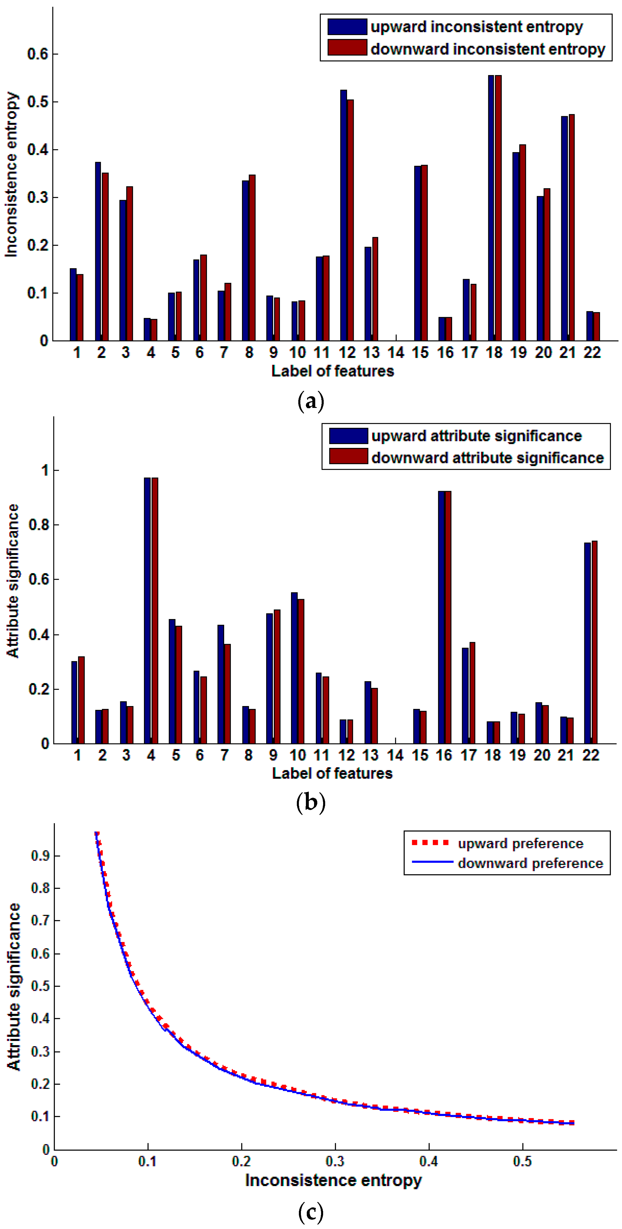
The Pasture Production data set was collected by Dave Barker from areas of grazed North Island hill country with recorded different management history during the period from 1793 to 1994. The objective was to analyze the influence of biophysical factors on pasture production. The Production of Pasture data set is composed of 36 tuples associated with 36 paddocks. Each tuple has 22 attributes, of which 19 are vegetation, and the others are soil chemical, physical and biological, and soil water variables, respectively. All the samples are partitioned into three classes, LO, MED and HI, representing low, medium and high production, respectively. Table 2 is the description of the features. For use in this work, we replaced these symbol values by integer 1, 2 and 3, respectively. Accordingly, the enumerated value (LL, LN, HN and HH) of attribute fertilizer are replaced by 1, 2, 3 and 4. Figure 1 shows the result of Experiment 1, Table 3 presents the selected features in the experiment, and the sample condensation result of Experiment 3 is listed in Table 4.

Table 2. Features of Pasture Production.

Sequence	Attribute	Description
1	fertiliser	{LL, LN, HN, HH}	enumerated
2	slope	Slope of the paddock	numeric
3	aspect-dev-NW	The deviation from the north-west	numeric
4	olsenP		numeric
5	minN		numeric
6	TS		numeric
7	Ca-Mg	Calcium magnesium ration	numeric
8	LOM	Soil lom (g/100g)	numeric
9	NFIX-mean	A mean calculation	numeric
10	Eworms-main-3	Main 3 spp earth worms per g/m2	numeric
11	Eworms-No-species	Number of spp	numeric
12	KUnSat	mm/h	numeric
13	OM		numeric
14	Air-Perm		numeric
15	Porosity		numeric
16	HFRG-pct-mean	Mean percent	numeric
17	legume-yield	kgDM/ha	numeric
18	OSPP-pct-mean	Mean percent	numeric
19	Jan-Mar-mean-TDR		numeric
20	Annual-Mean-Runoff	In mm	numeric
21	root-surface-area	M2/m3	numeric
22	Leaf-P	Ppm	numeric
Class	Pasture prod-class	{Low, Median, High}	enumerated

Figure 1. Preference inconsistence entropy and attribute significance of single features (Pasture production). (a) Inconsistent entropy of single features; (b) Significance of single features; (c) Relation of inconsistence entropy and attribute significance.

Table 3. Selected features for Pasture Production (original data set).

Data Set	Algorithm	Preference	Selected Features Subset	Significance of Feature Subset	Inconsistence Entropy of Feature Subset
Data set 1	Forward Feature Selection	upward	4, 11, 1	0.97, 0.25, 0.29	0
		downward	4, 11, 1	0.97, 0.24, 0.31	0
	Backward Feature Selection	upward	17, 18, 20, 22	0.4, 0.10, 0.19, 0.97	0
		downward	17, 18, 20, 22	0.48, 0.10, 0.17, 0.97	0
Data set 2	Forward Feature Selection	upward	4, 11, 22	0.36, 0.27, 0.97	0
		downward	4, 11, 22	0.32, 0.26, 0.97	0
	Backward Feature Selection	upward	5, 4, 3, 1	0.10, 0.15, 0.19, 0.97	0
		downward	5, 4, 3, 1	0.10, 0.13, 0.17, 0.97	0
Data set 3	Backward Feature Selection	upward	10, 16, 4	0.55, 0.92, 0.97	0
		downward	10, 16, 4	0.52, 0.92, 0.97	0
Data set 4	Forward Feature Selection	upward	4, 11, 16	0.97, 0.25, 0.92	0
		downward	4, 11, 16	0.97, 0.24, 0.92	0

Table 4. Selected samples (Pasture Production).

Features Subset	Upward Preference	Downward Preference
All features	2,4,7,8,9,10,11,12,13,14,15,16, 18,19,20,21,22,26,27,28,33,35	1,2,3,4,5,6,7,8,12,17,22,23, 24,25,28,29,30,31,32,34,35,36
4,11,1	2,9,10,11,12,13,14,15,16,18,19,20, 21,22,26,27,28,29,30,31,32,33,34,35,36	1,2,3,4,5,6,7,8,23,24,25, 28,29,30,31,32,34,35,36
4,11,22	2,4,7,8,9,10,11,12,13,14,15,16, 18,19,20,21,22,26,27,28,33,35	1,2,3,4,5,6,7,8,12,17,22,23, 24,25,28,29,30,31,32,34,35,36
17,18,20,22	1,2,4,7,8,9,10,11,12,13,14,15, 16,18,19,20,21,22,26,27,28,33,35	1,2,3,4,5,6,7,8,12,17,22,23, 24,25,28,29,30,31,32,34,35,36
1,3,4,5	5,9,10,11,12,13,14,15,16,18, 20,21,24,25,26,31,32,33,34,35,36	1,2,4,6,11,12,19,20,21,22,23, 24,25,28,29,30,31,32,34,35,36
10,16,4	2,3,4,8,9,10,11,12,13,14,15,16, 18,20,21,26,27,29,31,32,33,34,35,36	1,3,5,6,7,17,18,19,22,23,24, 25,28,29,30,31,32,34,35,36
4,11,16	2,5,6,7,9,10,11,12,13,14,15,16,18,20, 21,22,23,24,25,26,28,29,30,31,32,34,35,36	1,2,3,4,5,6,7,8,10,14,17,19,22,23, 24,25,27,28,29,30,31,32,33,34,35,36

Figure 1a shows the inconsistence entropy comparison of single features based on upward and downward preference. Figure 1b shows the comparison of signification of single features based on upward and downward preference. The relation of inconsistence entropy and attribute significance is presented in Figure 1c.

The inconsistence entropy of every feature of the decision is different, which shows that those features are not of the same importance in predicting pasture production. The inconsistence entropy monotonically decreases with increasing feature significance. The greater the inconsistence entropy is, the less the feature helps predict the pasture production, but in some cases, exceptions also exist.

We arrange these features in descending order by upward significance {4, 16, 22, 10, 9, 5, 7, 17, 1, 6, 11, 13, 3, 20, 8, 15, 2, 19, 21, 12, 18, 14}, and arrange the features in ascending order by upward inconsistence entropy {14, 4, 16, 22, 10, 9, 5, 7, 17, 1, 6, 11, 13, 3, 20, 8, 15, 2, 19, 21, 12, 18}. Except for feature 14, those attributes at the head of the first series have smaller inconsistence entropy and greater significance in predicting pasture production, such as 4, 16, 22, and so on. Feature 14 is an exception. The inconsistence entropy of feature 14 is the smallest value 0, but its significance also has the smallest value of 0. We can find that all distances have the same value 0 in feature 14, so its inconsistence entropy is 0. But at the same time, feature 14 is not different for all samples and cannot reflect any preference, so the significance should be 0. This is consistent with our common knowledge. The forward feature selection algorithm output the same features for upward preference and downward preference. As for the backward method, a similar case occurs.

In addition, from Figure 1, we can see that there is little difference between upward inconsistence entropy and downward inconsistence entropy. A similar case occurs for the significance of a single feature. In order to test how much the order of features impacts the output, we generated four different data sets by arranging the features in different order and executing the feature selection algorithms in all the data sets. All the features are labeled as 1, 2, ..., 22. The original data set is the first one. By arranging those features in a descending label order, we get the second data set. We compute the significance of every feature and get the third and the fourth data sets by arranging the features in the order of ascending and descending attribute significance, respectively. The forward algorithm is performed on data sets 1, 2 and 4, and the backward algorithm is executed on data sets 1, 2 and 3. Table 3 shows the experiment results.

For the forward algorithm, features 4, 11 and 1 are selected from data set 1, features 4, 11 and 1 are selected from data set 2, and features 4, 11 and 22 are selected from data set 4. Features 4 and 11 are included in all feature subset. The top two of three selected features are the same and only the last is different for all data sets. As for the backward algorithm, however, we have an entirely different situation. Features 17, 18, 20 and 22 are selected from data set 1, features 1, 3, 4 and 5 are selected from data set 2, and features 4, 10 and 16 are selected from data set 3. The selected feature subsets are totally different. Obviously, we can conclude that the forward algorithm is more stable and the backward algorithm is affected more by the order of features.

In the forward feature selection algorithm, the relative significance is computed in turn in the order of increasing feature label. As for the backward method, we compute the relative significance of features in the same turn. However, there exists an essential difference between the algorithms. For the forward algorithm, after the significances of all features are computed, the feature with maximal relative significance is selected, but for the backward method, if the relative significance is 0, the feature is immediately deleted from the features set. From Table 3, we can find that we can get similar feature subsets if we sort the data set by attribute significance. The backward algorithm selects features 4, 16 and 10 from data set 3 and the forward algorithm selects features 4, 16 and 11. We can see that features 4 and 16 appear in both the subsets. This shows that these features are important in term of different selection methods.

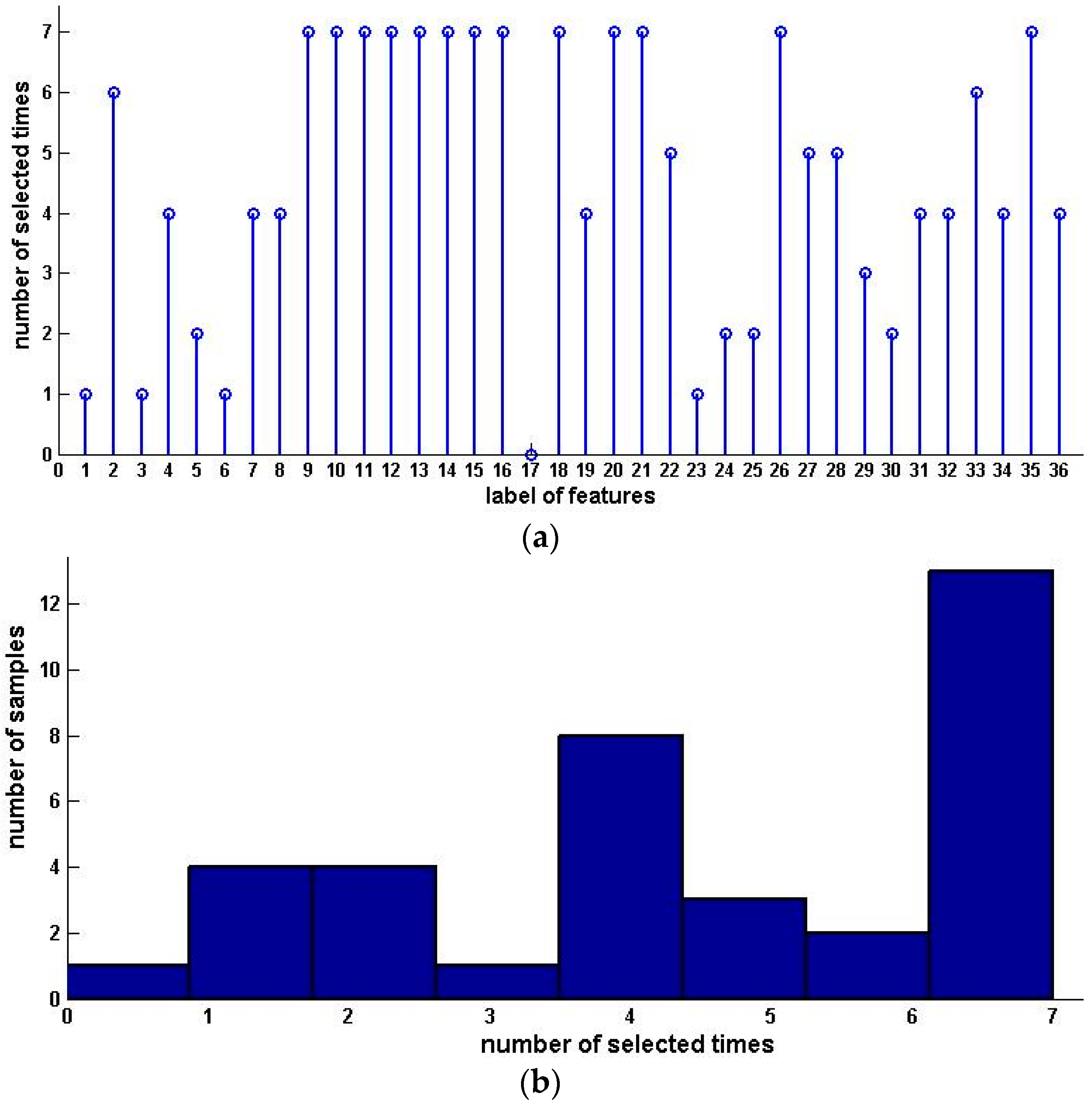
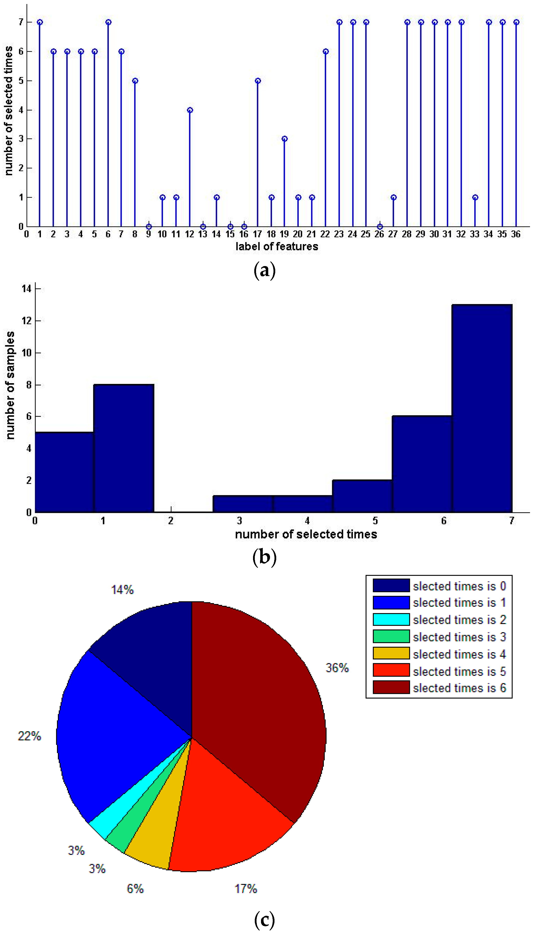
Table 4 shows the sample condensation results based on selected feature subsets in previous experiments. Figure 2 illustrates the distribution, histogram and pie of selected samples for upward preference. Figure 3 illustrates the distribution, histogram and pie of selected samples for downward preference.

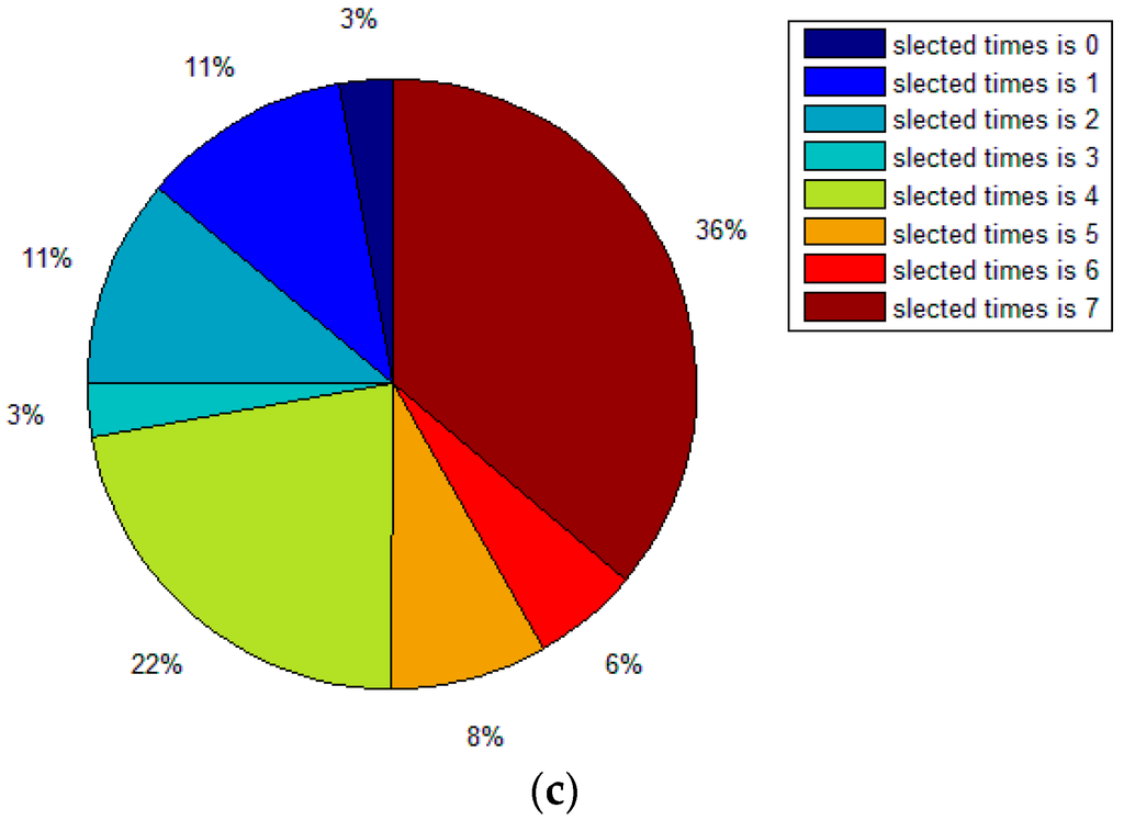
Figure 2. Distribution, histogram and pie of selected samples for upward preference (Pasture Production). (a) Distribution of selected samples; (b) Histogram of selected samples; (c) Pie of selected samples.

Figure 3. Distribution, histogram and pie of selected samples for downward preference (Pasture Production). (a) Distribution of selected samples; (b) Histogram of selected samples; (c) Pie of selected samples.

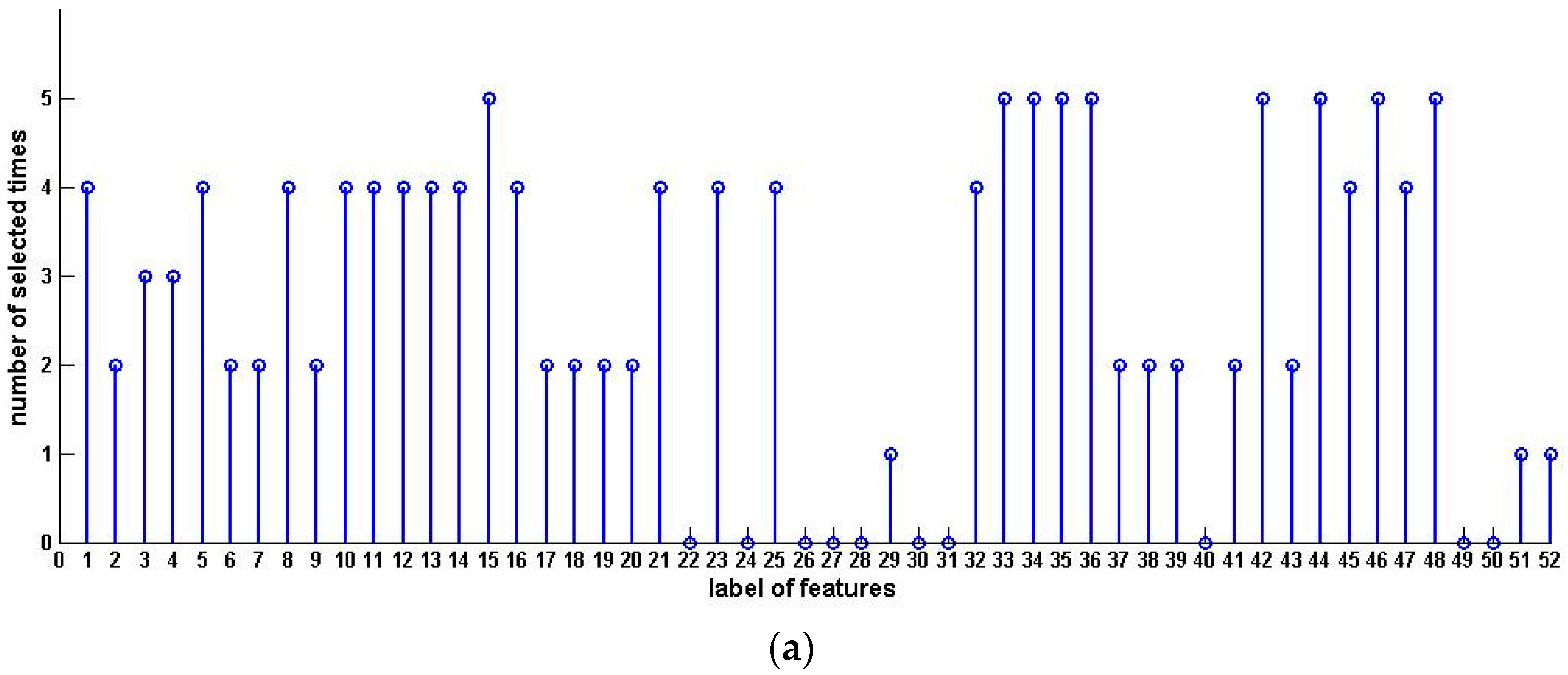
The Squash Harvest data set, collected by Winna Harvey Crop & Food Research (Christchurch, New Zealand), aims to determine which pre-harvest variables are important to good tasting squash after different periods of storage time so as to pinpoint the best time to give the best quality at the marketplace. This is determined by whether a measure of acceptability found by classifying each squash as either unacceptable, acceptable or excellent. The name and the corresponding descriptions of those features are described in Table 5. There are 52 instances with 24 attributes. For use in this work, we replaced these class symbol values with integer 1, 2 and 3, respectively. We do the same tests on this data set.

Table 5. Features of Squash Harvest.

Sequence	Attribute	Description
1	site	where fruit is located	enumerated
2	daf	number of days after flowering	enumerated
3	fruit	individual number of the fruit	enumerated
4	weight	weight of whole fruit in grams	numeric
5	storewt	weight of fruit after storage	numeric
6	pene	penetrometer indicates maturity of fruit at harvest	numeric
7	solids_%	a test for dry matter	numeric
8	brix	a refactometer measurement used to indicate sweetness or ripeness of the fruit	numeric
9	a*	the a* coordinate of the HunterLab L*, a*, b* notation of color measurement	numeric
10	egdd	the heat accumulation above a base of 8c from emergence of the plant to harvest of the fruit	numeric
11	fgdd	the heat accumulation above a base of 8c from flowering to harvesting	numeric
12	ground spot	the number indicating color of skin where the fruit rested on the ground	numeric
13	glucose	measured in mg/100g of fresh weight	numeric
14	fructose	measured in mg/100g of fresh weight	numeric
15	sucrose	measured in mg/100g of fresh weight	numeric
16	total	measured in mg/100g of fresh weight	numeric
17	Glucose + fructos	measured in mg/100g of fresh weight	numeric
18	starch	measured in mg/100g of fresh weight	numeric
19	sweetness	the mean of eight taste panel scores	numeric
20	flavour	the mean of eight taste panel scores	numeric
21	dry/moist	the mean of eight taste panel scores	numeric
22	fibre	the mean of eight taste panel scores	numeric
23	heat_input_emerg	the amount of heat emergence after harvest	numeric
24	heat_input_flower	the amount of heat input before flowering	numeric
25	acceptability	the acceptability of the fruit	enumarated

We compute the inconsistence entropy and attribute significance of single features for upward preference and downward preference, as shown in Figure 4. Features 1, 2, 6, 11, 16 and 24 have greater single attribute significance, indicating that, as far as single features are concerned, site, number of days after flowering, maturity of fruit at harvest, the heat accumulation from flowering to harvesting, total number of glucose, fructose and sucrose and the amount of heat input before flowering are very important for good taste.

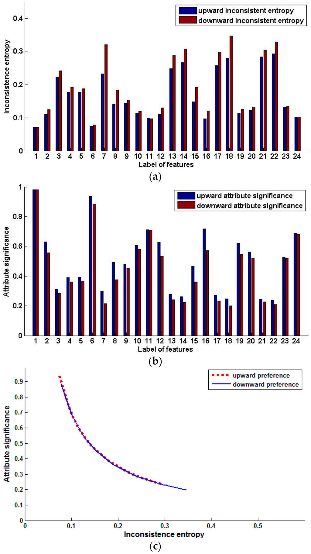
Figure 4. Preference inconsistence entropy and attribute significance of single features (Squash Harvest). (a) Inconsistence entropy of single features; (b) Significance of single features; (c) Relation of attribute significance and inconsistence entropy.

We also extract the preference consistence feature subset. Similar to Pasture Production, we generate four data sets from Squash Harvest. All the features are labeled as 1, 2, ..., 24. The original data set is the first. By arranging those features in the order of descending label, we get the second data set.

We compute the significance of every feature and get the third and the fourth data sets by arranging the features in the order of ascending and descending attribute significance, respectively. The forward algorithm is performed on data sets 1, 2 and 4, and the backward algorithm is executed on data sets 1, 2 and 3. Table 6 shows the experiment results. Finally, we condense the samples with selected features. The results are shown in Table 7. Figure 5 and Figure 6 show the distribution and histograms of selected samples.

Table 6. Selected features for Squash Harvest (original data set).

Data Set	Algorithm	Preference	Selected Features Subset	Significance of Feature Subset	Inconsistent Entropy of Feature Subset
Original data	Forward Feature Selection	upward	1, 2, 14	0.98, 0.63, 0.26	0
		downward	1, 2, 14	0.98, 0.55, 0.22	0
	Backward Feature Selection	upward	15, 17, 18, 22, 24	0.66, 0.38, 0.35, 0.33, 0.98	0
		downward	15, 17, 18, 22, 24	0.66, 0.38, 0.35, 0.33, 0.98	0
Sorted by feature label descending	Forward Feature Selection	upward	1, 2, 14	0.98, 0.63, 0.26	0
		downward	1, 2, 14	0.98, 0.55, 0.22	0
	Backward Feature Selection	upward	9, 3, 2, 1	0.98, 0.32, 0.72, 0.94	0
		downward	9, 3, 2, 1	0.82, 0.30, 0.75, 0.98	0
Sorted by significance descending	Forward Feature Selection	upward	1, 2, 14	0.98, 0.63, 0.26	0
		downward	1, 2, 14	0.98, 0.55, 0.22	0
Sorted by significance ascending	Backward Feature Selection	upward	8, 12, 2, 16, 1	0.49, 0.62, 0.63, 0.71, 0.98	0
		downward	8, 12, 2, 16, 1	0.37, 0.53, 0.55, 0.57, 0.98	0

Table 7. Selected samples (Squash Harvest).

Features subset	Upward Preference	Downward Preference
All features	1,5,8,10,11,12,13,14,15,16,21,23, 25,32,33,34,35,36,42,44,45,46,47,48	1,2,6,7,9,12,13,14,15,16,22,24,26,27,28,29, 30,31,33,34,35,36,37,38,39,40,49,50,51,52
1,2,14	1,3,4,15,33,34,35,36,42,44,46,48,52	1,2,6,7,9,12,13,14,15,16,22,24, 26,27,28,29,30,31,40,49,50,51,52
15,17,18,22,24	5,8,10,11,12,13,14,15,16,21,23, 25,32,33,34,35,36,42,44,45,46,47,48	1,2,6,7,9,12,13,14,15,16,22,24,26,27,28, 29,30,31,33,34,35,36,37,38,39,40,49,50,51,52
9,3,2,1	1,2,3,4,5,6,7,8,9,10,11,12,13,14,15,16, 17,18,19,20,21,23,25,32,33,34,35,36, 37,38,39,41,42,43,44,45,46,47,48,51	1,2,6,7,9,12,13,14,15,16,22,24,26,27, 28,29,30,31,33,34,35,36,37,38,39,40, 41,42,43,44,45,46,47,48,49,50,51,52
8,12,2,16,1	1,2,3,4,5,6,7,8,9,10,11,12,13,14,15,16, 17,18,19,20,21,23,25,29,32,33,34,35, 36,37,38,39,41,42,43,44,45,46,47,48	1,2,6,7,9,12,13,14,15,16,22,24,26,27, 28,29,30,31,33,34,35,36,37,38,39,40, 41,42,43,44,45,46,47,48,49,50,51,52

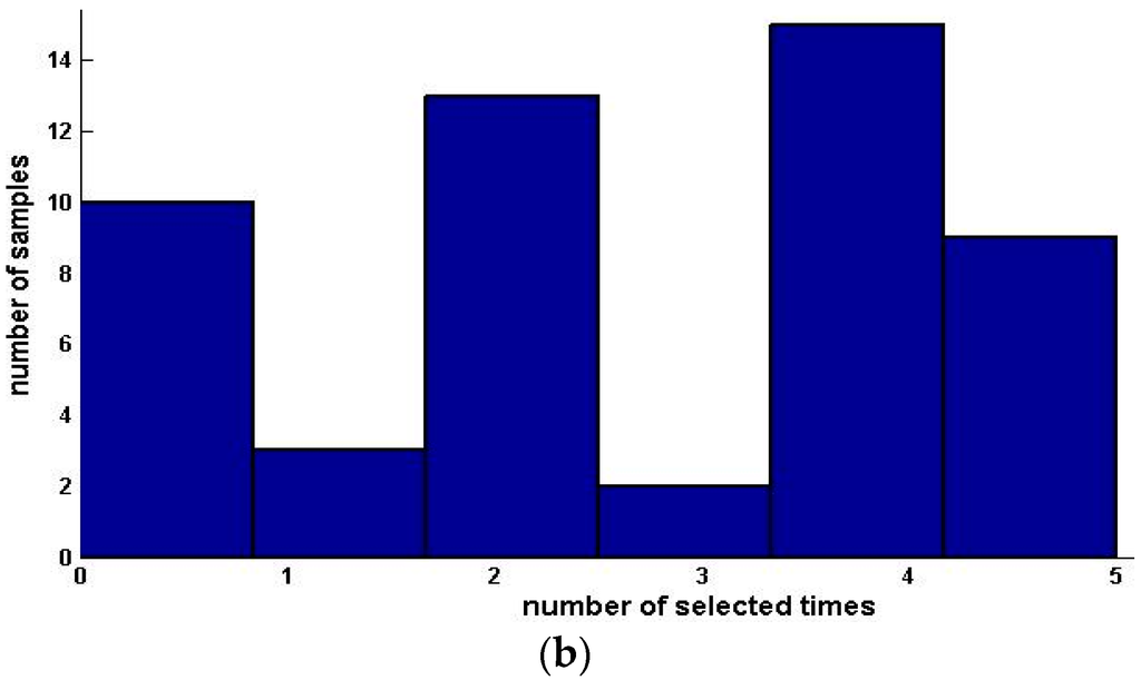
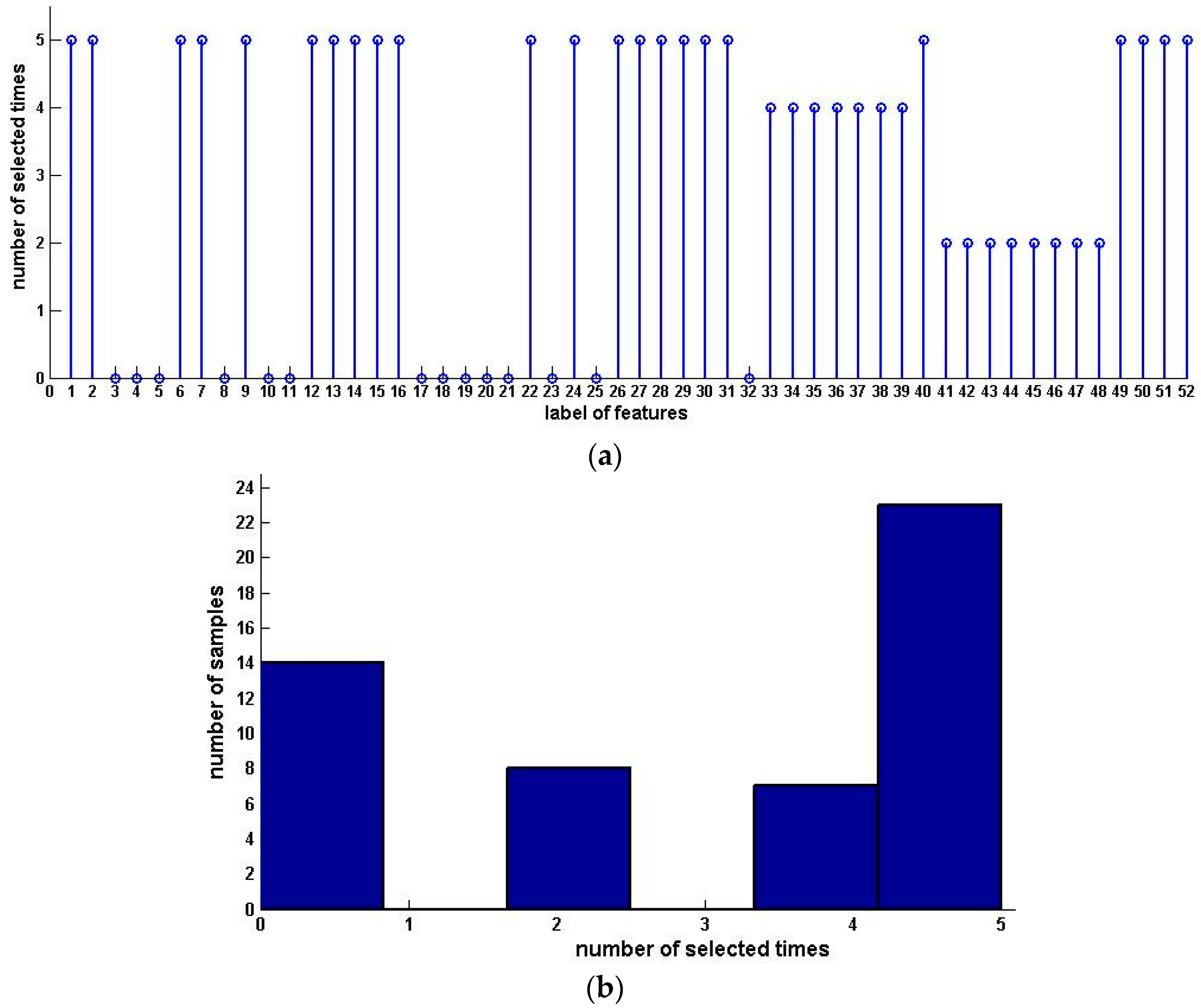
Figure 5. Distribution, histogram and pie of selected samples for upward preference (Squash Harvest). (a) Distribution of selected samples; (b) Histogram of selected samples.

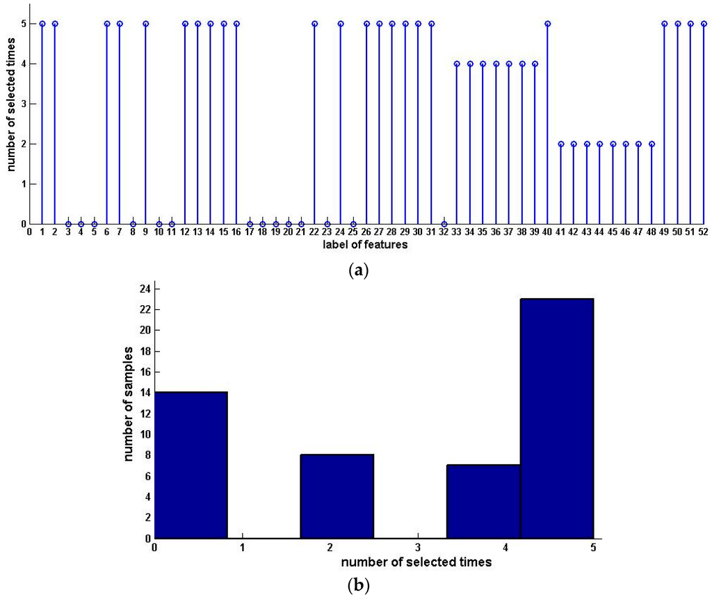
Figure 6. Distribution and histogram of selected samples for downward preference (Squash Harvest). (a) Distribution of selected samples; (b) Histogram of selected samples.

For the forward algorithm, we get the same feature subset 1, 2 and 14. The attribute significance of features 1 is 0.98. Feature 2 has an attribute significance of 0.63 and 0.55 for upward preference and downward preference, respectively. Features 1 and 2 are important for good taste, but the significance of feature 14 is as low at 0.26 and 0.22 for upward preference and downward preference, respectively. This indicates that, more glucose can give better taste at harvest if the plant site is suitable and the number of days after flowering is enough.

6. Conclusions

In multiple attribute ordinal decision, the derived decisions may be inconsistent and uncertain since the available information is usually obtained from different evaluation criteria or experts. Shannon entropy is a suitable measurement of uncertainty. In this research, Shannon entropy is extended to preference inconsistence entropy for preference inconsistent ordinal decision systems. Two applications of preference inconsistence entropy, feature selection and sample condensation, are addressed and some algorithms are developed. The experimental result shows that preference inconsistence entropy is a suitable measurement of uncertainty of preference decision, and the proposed algorithms are effective solutions for preference analysis. Classification is another interesting issue for preference analysis, and further investigations on classification methods and algorithms based on preference inconsistence entropy are worthwhile.

References

- Lotfi, F.H.; Fallahnejad, R. Imprecise Shannon’s entropy and multi attribute decision making. Entropy 2010, 12, 53–62. [Google Scholar] [CrossRef]
- Saaty, T.L. The Analytic Hierarchy Process; McGraw-Hill: New York, NY, USA, 1980. [Google Scholar]
- Chu, A.T.W.; Kalaba, R.E.; Spingarn, K. A comparison of two methods for determining the weights of belonging to fuzzy sets. J. Optim. Theory Appl. 1979, 27, 531–538. [Google Scholar] [CrossRef]
- Hwang, C.-L.; Lin, M.-J. Group Decision Making under Multiple Criteria: Methods and Applications; Springer: Berlin/Heidelberg, Germany, 1987. [Google Scholar]
- Choo, E.U.; Wedley, W.C. Optimal criterion weights in repetitive multicriteria decision-making. J. Oper. Res. Soc. 1985, 36, 983–992. [Google Scholar] [CrossRef]
- Fan, Z.P. Complicated Multiple Attribute Decision Making: Theory and Applications. Ph.D. Thesis, Northeastern University, Shenyang, China, 1996. [Google Scholar]
- Moshkovich, H.M.; Mechitov, A.I.; Olson, D.L. Rule induction in data mining: Effect of ordinal scales. Expert Syst. Appl. 2002, 22, 303–311. [Google Scholar] [CrossRef]
- Harker, P.T. Alternative modes of questioning in the analytic hierarchy process. Math. Model. 1987, 9, 353–360. [Google Scholar] [CrossRef]
- Saaty, T.L.; Vargas, L.G. Uncertainty and rank order in the analytic hierarchy process. Eur. J. Oper. Res. 1987, 32, 107–117. [Google Scholar] [CrossRef]
- Xu, Z.S. Method for group decision making with various types of incomplete judgment matrices. Control Decis. 2006, 21, 28–33. [Google Scholar]
- Van Laarhoven, P.J.M.; Pedrycz, W. A fuzzy extension of Saaty’s priority theory. Fuzzy Sets Syst. 1983, 11, 199–227. [Google Scholar] [CrossRef]
- Luce, R.D.; Suppes, P. Preferences Utility and Subject Probability. In Handbook of Mathematical Psychology; Luce, R.D., Bush, R.R., Galanter, E.H., Eds.; Wiley: New York, NY, USA, 1965; Volume 3, pp. 249–410. [Google Scholar]
- Alonso, S.; Chiclana, F.; Herrera, F.; Herrera-Viedma, E. A Learning Procedure to Estimate Missing Values in Fuzzy Preference Relations Based on Additive Consistency. In Modeling Decisions for Artificial Intelligence; Springer: Berlin/Heidelberg, Germany, 2004; pp. 227–238. [Google Scholar]
- Xu, Z.S. A practical method for priority of interval number complementary judgment matrix. Oper. Res. Manag. Sci. 2002, 10, 16–19. [Google Scholar]
- Herrera, F.; Herrera-Viedma, E.; Verdegay, J.L. A model of consensus in group decision making under linguistic assessments. Fuzzy Sets Syst. 1996, 78, 73–87. [Google Scholar] [CrossRef]
- Herrera, F.; Herrera-Viedma, E.; Verdegay, J.L. Direct approach processes in group decision making using linguistic OWA operators. Fuzzy Sets Syst. 1996, 79, 175–190. [Google Scholar] [CrossRef]
- Greco, S.; Matarazzo, B.; Slowinski, R. Rough approximation of a preference relation by dominance relations. Eur. J. Oper. Res. 1999, 117, 63–83. [Google Scholar] [CrossRef]
- Greco, S.; Matarazzo, B.; Slowinski, R. Rough approximation by dominance relations. Int. J. Intell. Syst. 2002, 17, 153–171. [Google Scholar] [CrossRef]
- Hu, Q.H.; Yu, D.R.; Guo, M.Z. Fuzzy preference based rough sets. Inf. Sci. 2010, 180, 2003–2022. [Google Scholar] [CrossRef]
- Abbas, A.E. Entropy methods for adaptive utility elicitation. IEEE Trans. Syst. Man Cybern. 2004, 34, 169–178. [Google Scholar] [CrossRef]
- Yang, J.; Qiu, W. A measure of risk and a decision-making model based on expected utility and entropy. Eur. J. Oper. Res. 2005, 164, 792–799. [Google Scholar] [CrossRef]
- Abbas, A.E. Maximum Entropy Utility. Oper. Res. 2006, 54, 277–290. [Google Scholar] [CrossRef]
- Abbas, A. An Entropy Approach for Utility Assignment in Decision Analysis. In Proceedings of the 22nd International Workshop on Bayesian Inference and Maximum Entropy Methods in Science and Engineering, Moscow, Russian Federation, 3–9 August 2002; pp. 328–338.
- Hu, Q.H.; Yu, D.R. Neighborhood Entropy. In Proceedings of the 2009 International Conference on Machine Learning and Cybernetics, Baoding, China, 12–15 July 2009; Volume 3, pp. 1776–1782.
- Jaynes, E.T. Information theory and statistical mechanics II. Phys. Rev. 1957, 108, 171–190. [Google Scholar] [CrossRef]
- Kullback, S.; Leibler, R.A. On information and sufficiency. Ann. Math. Stat. 1951, 22, 79–86. [Google Scholar] [CrossRef]
- Kullback, S. Information Theory and Statistics; Wiley: New York, NY, USA, 1959. [Google Scholar]
- Hu, Q.H.; Che, X.J.; Zhang, L.D.; Guo, M.Z.; Yu, D.R. Rank entropy based decision trees for monotonic classification. IEEE Trans. Knowl. Data Eng. 2012, 24, 2052–2064. [Google Scholar] [CrossRef]
- Jaynes, E.T. Information theory and statistical mechanics. Phys. Rev. 1957, 106, 620–630. [Google Scholar] [CrossRef]
- Shannon, C.E. A mathematical theory of communication. Bell Syst. Tech. J. 1948, 27, 379–423, 623–656. [Google Scholar] [CrossRef]
- Zeng, K.; Kun, S.; Niu, X.Z. Multi-Granulation Entropy and Its Application. Entropy 2013, 15, 2288–2302. [Google Scholar] [CrossRef]
© 2016 by the authors; licensee MDPI, Basel, Switzerland. This article is an open access article distributed under the terms and conditions of the Creative Commons by Attribution (CC-BY) license (http://creativecommons.org/licenses/by/4.0/).