Entropy Complexity and Stability of a Nonlinear Dynamic Game Model with Two Delays

Abstract

In this paper, a duopoly game model with double delays in hydropower market is established, and the research focus on the influence of time delay parameter on the complexity of the system. Firstly, we established a game model for the enterprises considering both the current and the historical output when making decisions. Secondly, the existence and stability of Hopf bifurcation are analyzed, and the conditions and main conclusions of Hopf bifurcation are given. Thirdly, numerical simulation and analysis are carried out to verify the conclusions of the theoretical analysis. The effect of delay parameter on the stability of the system is simulated by a bifurcation diagram, the Lyapunov exponent, and an entropic diagram; in addition, the stability region of the system is given by a 2D parameter bifurcation diagram and a 3D parameter bifurcation diagram. Finally, the method of delayed feedback control is used to control the chaotic system. The research results can provide a guideline for enterprise decision-making.

1. Introduction

As the demand for power increases, the supply is proportionately increased. However, the cost of thermal power, which is generated by non-renewable resources, is extremely high. Therefore, the development of hydroelectric power is a more sensible choice. In this paper, the game process of power output of two hydropower enterprises is considered. In practice, there is an obvious relationship between the amount of electricity generated and the amount of water reserves. As a result, the water reserves, the current output, and the output of the time delay are mainly considered to make an electricity output plan. Therefore, it is very meaningful to study the game competition of the electricity output of the two-oligopoly enterprises.

Electricity is an energy source of great significance, related to country development and societal stability, so has always been the focus of research. As for studies on energy in relation to economic strategies and the environment, Weidou [1] analyzed China’s energy policies and provided reasonable suggestions for the supply and consumption of China’s energy, which would ensure the sustainable development of China’s social energy economy. Nwaobi [2] proposed an economic model based on the emission reduction policy, and gave an empirical analysis of Nigeria as an example. Vera et al. [3] are in the process of analyzing the problem of 3E. They established a national energy index system to develop the energy policy and realize the sustainable development of society, the economy, the environment, and energy. Omri [4] analyzed the relationship between economic growth and a group of parameters: energy consumption, electricity consumption, nuclear consumption, and renewable energy consumption.

In recent years, the oligopoly game has always been the frontier research area of renewable energy, especially the nonlinear dynamic model, which is closely related to real life. Using the entropy theory and chaos theory to establish an oligopolistic competition game model, establishing a measuring method for uncertainty, and eliminating uncertainty all have broad applicability.

Dajka et al. [5] considered a two-player quantum game in the presence of a thermal decoherence modeled in terms of a rigorous Davies approach. This shows how the energy dissipation and pure decoherence affect the payoffs of the players of the game. Harré et al. [6] considered the issue about how changes in the underlying incentives can move us from an optimal economy to a sub-optimal economy, meanwhile making it impossible to collectively navigate our way to a better strategy without forcing us to pass through a socially undesirable “tipping point”.

The power market of the three-oligopoly game was analyzed by Ma [7], where the complex dynamic characteristics of the system are studied, and the dynamic behavior of the game is given, providing an excellent practical guideline that is of great significance. Batabyal [8] took the international trade of renewable resources as the background, did corresponding analysis using the Stackelberg differential model, and pointed out that the policy tool has an important role in promoting energy conservation. This study has important implications for the conservation of renewable energy. As for the Bertrand model, Sun et al. [9] proposed a three-oligopoly game model, which is based on the cold rolling market of China and studied the complex dynamic characteristics of the game process. Basing on the Markov information structure, Halkos et al. [10] put forward a renewable energy and non-renewable energy Nash game, and carried out the analysis of its strategy by using the utility function, which is of great significance in practice. Liao [11] analyzed the role of developing hydro-energy, wind energy, nuclear power, and so forth. Yoon and Ratti [12] examined the effect of energy price uncertainty on firm-level investment with data on U.S. manufacturing firms.

Chaos analysis and applications in dynamical systems are observed in many practical applications in engineering, biology, and economics [13,14,15]. Sun and Tian established an energy resource demand-supply system based on the background of the real energy resources demand and supply in the East and the West of China [16], and have obtained a series of findings [17,18].

In this paper, we study the problem of the oligopoly game in the market of hydroelectric power using nonlinear theory and complex dynamics theory. We analyze the complex dynamic characteristics of the system and study the influence of the time delay and weight on the system. Moreover, an effective method for controlling a chaotic system is carried out.

This paper is organized as follows. In Section 2, a continuous differential duopoly game mode with two delays is established. In Section 3, we focus on analyzing the existence and stability of Hopf bifurcation. In Section 4, we carry out numerical simulation and analysis by using the methods of the attractor, bifurcation diagram, Lyapunov exponent, entropic, etc. to study the influence of delay and weight on the stability of the system. In Section 5, we elaborate on delayed feedback control, which is an effective control method of chaos. Finally, the conclusions of this paper are given in Section 6.

2. The Model

In the market of hydroelectric power, we want to find the total economic variables: electrovalence, market demand, and water reserves. The conditions need to be met when the market reaches equilibrium. So, in this paper, we focus on the influence of the time delay parameter on the dynamic characteristics of the system.

Assumptions are listed as follows:

• The electricity market is composed of two hydropower enterprises.
• The output of electricity quantity is only related to the amount of water reserves and electrovalence.
• Electricity price is determined by the output of electricity quantity of two enterprises and social demand.
• In order to generate electricity and ensure water storage safety, the minimum water reserve is $X_{\min }$ the maximum water reserve is $X_{\max }$. Therefore, the water reserves $X$ must satisfy $X\in ({\mathrm{X}}_{\min },{\mathrm{X}}_{\max })$.

The inverse demand function for the electricity market is $p(q)=\overline{p}-q$, where $p$ is electrovalence, $q={\displaystyle \sum _{i=1}^N{q}_i}$ is the demand of electrical energy, and $\overline{p}$ is the highest price of the electrical energy [9].

In the electricity market, the cost function $C(X)$ is related to its own water reserves $X$ [10,11]. $X_{\min }$ is the water reserve when $C(X_{\min })=\overline{p}$. Obviously, $x=X-X_{\min }$ is the effective water reserve. When $X\le X_{\min }$, hydro power stations will suspend power generation. The unit cost of water reserves is $c(x)=\overline{p}-cx$. If water is renewable, and the growth rate of the water reserve is $k$, then $\dot{x}=kx$. So, the water reserves should meet $\dot{x}=kx-q$.

In the process of the market game, every player in the game has to achieve its own profit maximization:

$$\pi =\left[p(q)-c(x_i)\right]q_i=\left(c{x}_i-q\right)q_i.$$

So, the problem of the game strategy for each oligopoly can be expressed as the optimization problem:

$$\underset{q_i}{\max }{{\displaystyle \int }}_0^{\infty }{e}^{-\theta t}(c{x}_i-q)q_{i}dt$$

(1)

$$s.t.\hspace{1em}{\dot{x}}_i=k{x}_i-q_i,$$

(2)

where $\theta$ is discount factor, $\theta >0$, $q_i\ge 0$, $x_i\ge 0$ and $i=1,2$.

Solving the optimization problem (1) with its Hamiltonian function:

$$H^i=(c{x}_i-q^2)q_i+{\lambda }_i(k{x}_i-q_i),$$

(3)

where ${\lambda }_i$ is a co-state variable. Solving:

$$\frac{\partial H^i}{\partial q_i}=0, {\dot{\lambda }}_i=-\frac{\partial H^i}{\partial x_i}+\theta {\lambda }_i.$$

Simultaneously we can obtain:

$${\dot{q}}_i+\dot{q}=(\theta -k)({\dot{q}}_i+\dot{q})+c(2k-\theta )x_i, i=1,2.$$

(4)

The sum of the two parts of Equation (4) is obtained, and, using $q={\displaystyle \sum _{i=1}^N{q}_i}$ and $x={\displaystyle \sum _{i=1}^N{x}_i}$ $(N=2)$, we can derive:

$$\dot{q}=(\theta -k)q+\frac{c(2k-\theta )}{N+1}x.$$

(5)

With Equations (4) and (5), we can calculate the game strategy for each oligopoly as:

$${\dot{q}}_i=(\theta -k)q_i+c(2k-\theta )x_i-\frac{c(2k-\theta )}{3}x.$$

(6)

In the actual operation of the electricity market, in order to ensure the sustainable development of electric energy, as well as the stability of the electrovalence, the electricity supply of the market should be fixed in a certain period of time, to ensure that the supply of electricity is not too large or too small, which leads to fluctuations in market price. Suppose that in a certain period of time, the largest electricity supply is $a$, so ${\dot{q}}_i$ positive correlation with $v_i(a-q)$, $v_i$ is the change rate of electricity supply.

Therefore, integrating Equations (5) and (6) and $v_i(a-q)$, we can obtain a double oligopoly game model for the hydroelectric power market:

$$\{\begin{array}{l}{\dot{x}}_1=k{x}_1-q_1\\ {\dot{x}}_2=k{x}_2-q_2\\ {\dot{q}}_1=v_1(a-q_2-q_1)\left[(\theta -k)q_1-c(2k-\theta )x_2+\frac{2}{3}c(2k-\theta )x_1\right]\\ {\dot{q}}_2=v_2(a-q_1-q_2)\left[(\theta -k)q_2-c(2k-\theta )x_1+\frac{2}{3}c(2k-\theta )x_2\right]\end{array}.$$

(7)

In the actual operation process of the electric power enterprise, it is not only necessary to consider the current market demand; we also need to consider the market demand of $\tau$ time early, which makes the final decision results closer to the actual situation. In this paper, we assume that the duopoly considers time delay. The delay parameters are ${\tau }_1$ and ${\tau }_2$ respectively. That is:

$$q_i(t)={\mu }_i{q}_i(t)+(1-{\mu }_i)q_i(t-{\tau }_i),$$

(8)

and $0<{\mu }_i<1$, $i=1,2$ is the weight of the current period price.

We know that the time delay does not affect the system’s solution. Therefore, the equilibrium point $E_{*}(0,0,0,0)$ of Equation (7) is also the equilibrium point with a time delay system. So, in this paper, we analyze the delay decision with the equilibrium point of $E_{*}(0,0,0,0)$. Then, from Equations (7) and (8), the linear system with time delay is:

$$\{\begin{array}{l}{\dot{x}}_1=k{x}_1-q_1,\\ {\dot{x}}_2=k{x}_2-q_2,\\ {\dot{q}}_1(t)=a{v}_1\left[(\theta -k)({\mu }_1{q}_1(t)+(1-{\mu }_1)q_1(t-{\tau }_1))-c(2k-\theta )x_2(t)+\frac{2}{3}c(2k-\theta )x_1(t)\right],\\ {\dot{q}}_2(t)=v_2(a-{\mu }_1{q}_1(t)-(1-{\mu }_1)q_1(t-{\tau }_1)-{\mu }_2{q}_2(t)-(1-{\mu }_2)q_2(t-{\tau }_2))\\ \left[(\theta -k)({\mu }_2{q}_2(t)+(1-{\mu }_2)q_2(t-{\tau }_2))-c(2k-\theta )x_1(t)+\frac{2}{3}c(2k-\theta )x_2(t)\right].\end{array}$$

(9)

3. Stability and Existence of Hopf Bifurcation

Equation (9) is linearized at the equilibrium point $E_{*}(0,0,0,0)$ by using s Jacobian matrix. So Equation (9) can be converted to:

$$\{\begin{array}{l}{\dot{x}}_1=k{x}_1-q_1,\\ {\dot{x}}_2=k{x}_2-q_2,\\ {\dot{q}}_1=A_1{q}_1(\mathrm{t})+B_1(1-{\mu }_1)q_1(\mathrm{t}-{\tau }_1)+C_1{x}_1(\mathrm{t})+D_1{x}_2(\mathrm{t}),\\ {\dot{q}}_2={\mu }_2{q}_2(\mathrm{t})+A_2(1-{\mu }_2)q_2(\mathrm{t}-{\tau }_2)-(a{\nu }_{2}M+M)x_1(\mathrm{t})+a{\nu }_{2}N{x}_2(\mathrm{t})\\ -B_2{\mu }_2{q}_1(\mathrm{t})q_2(\mathrm{t}) -B_2(1-{\mu }_2)q_1(\mathrm{t})q_2(\mathrm{t}-{\tau }_2)+{\nu }_2{\mu }_1{q}_1(\mathrm{t})-{\nu }_2{\mu }_1{q}_1(\mathrm{t})N{x}_2(\mathrm{t})\\ -C_2{\mu }_2{q}_1(\mathrm{t}-{\tau }_1)q_2(\mathrm{t})-C_2(1-{\mu }_2)q_1(\mathrm{t}-{\tau }_1)q_2(\mathrm{t}-{\tau }_2)+D_{2}M{q}_1(\mathrm{t}-{\tau }_1)x_1(\mathrm{t})\\ -D_{2}N{q}_1(\mathrm{t}-{\tau }_1)x_2(\mathrm{t})-E_2{q}_2{(\mathrm{t})}^2-E_2(1-{\mu }_2)q_2(\mathrm{t})q_2(\mathrm{t}-{\tau }_2)+{\nu }_2{\mu }_{2}M{q}_2(\mathrm{t})x_1(\mathrm{t})\\ -{\nu }_2{\mu }_{2}N{q}_2(\mathrm{t})x_2(\mathrm{t})-F_2{\mu }_2{q}_2(\mathrm{t})q_2(\mathrm{t}-{\tau }_2)-F_2(1-{\mu }_2)q_2{(\mathrm{t}-{\tau }_2)}^2\\ +G_{2}M{q}_2(\mathrm{t}-{\tau }_2)x_1(\mathrm{t})-G_{2}N{q}_2(\mathrm{t}-{\tau }_2)x_2(\mathrm{t}),\end{array}$$

(10)

where

$$A_1=a{\nu }_1{\mu }_1(\theta -\mathrm{k}), B_1=a{\nu }_1(\theta -\mathrm{k}), C_1=\frac{2}{3}ac{\nu }_1(2\mathrm{k}-\theta ),$$

$$D_1=-a{\nu }_{1}c(2\mathrm{k}-\theta ), M=c(2k-\theta ), N=\frac{2}{3}c(2k-\theta ), A_2=a{\nu }_2(\theta -k),$$

$$B_2={\nu }_2{\mu }_1(\theta -k), C_2={\nu }_2(1-{\mu }_1)(\theta -k), D_2={\nu }_2(1-{\mu }_1),$$

$$E_2={\nu }_2{\mu }_2(\theta -k), F_2={\nu }_2(1-{\mu }_2)(\theta -k), G_2={\nu }_2(1-{\mu }_2).$$

The characteristic equation of Equation (10) is

$$\begin{array}{l}{\lambda }^4+f_{13}{\lambda }^3+f_{12}{\lambda }^2+f_{11}\lambda +f_{10}+(f_{23}{\lambda }^3+f_{22}{\lambda }^2+f_{21}\lambda +f_{20}){\mathrm{e}}^{-\lambda {\tau }_1}\\ +(f_{33}{\lambda }^3+f_{32}{\lambda }^2+f_{31}\lambda +f_{30}){\mathrm{e}}^{-\lambda {\tau }_2}+(f_{42}{\lambda }^2+f_{41}\lambda +f_{40})e^{-\lambda ({\tau }_1+{\tau }_2)}=0\end{array},$$

(11)

where

$$f_{13}=-2k-{\mu }_2-A_1,$$

$$f_{12}=C_1+k^2+2A_{1}k+A_1{\mu }_2+2k{\mu }_2+Na{v}_2,$$

$$f_{11}=D_1{\mu }_1{v}_2-A_1{k}^2-k^2{\mu }_2-C_{1}k-C_1{\mu }_2-2A_{1}k{\mu }_2-Na{A}_1{v}_2-Nak{v}_2,$$

$$f_{10}=C_{1}k{\mu }_2-M{D}_1+A_1{k}^2{\mu }_2-C_{1}k{\mu }_1{v}_2-Ma{D}_1{v}_2+Na{C}_1{v}_2+Na{A}_{1}k{v}_2,$$

$$f_{23}=B_1{\mu }_1-B_1,$$

$$f_{22}=2B_{1}k-2B_{1}k{\mu }_1+B_1{\mu }_2-B_1{\mu }_1{\mu }_2,$$

$$f_{21}=B_1{k}^2{\mu }_1-B_1{k}^2-Na{B}_1{\nu }_2-2B_{1}k{\mu }_2+Na{B}_1{\mu }_1{\nu }_2+2B_{1}k{\mu }_1{\mu }_2,$$

$$f_{20}=B_1{k}^2{\mu }_2-B_1{k}^2{\mu }_1{\mu }_2+Na{B}_{1}k{v}_2-Na{B}_{1}k{\mu }_1{v}_2,$$

$$f_{33}=A_2{\mu }_2-A_2,$$

$$f_{32}=A_1{A}_2-2A_{2}k{\mu }_2+2A_{2}k-A_1{A}_2{\mu }_2,$$

$$f_{31}=-A_2{k}^2+A_2{k}^2{\mu }_2-A_2{C}_1-2A_1{A}_{2}k+2A_1{A}_{2}k{\mu }_2+A_2{C}_1{\mu }_2,$$

$$f_{30}=A_1{A}_2{k}^2+A_2{C}_{1}k-A_2{C}_{1}k\mu 2-A_1{A}_2{k}^2\mu 2,$$

$$f_{42}=A_2{B}_1+A_2{B}_1{\mu }_1{\mu }_2-A_2{B}_1{\mu }_1-A_2{B}_1{\mu }_2,$$

$$f_{41}=2A_2{B}_{1}k{\mu }_2-2A_2{B}_{1}k+2A_2{B}_{1}k{\mu }_1-2A_2{B}_{1}k{\mu }_1{\mu }_2,$$

$$f_{40}=A_2{B}_1{k}^2-A_2{B}_1{k}^2{\mu }_1-A_2{B}_1{k}^2{\mu }_2+A_2{B}_1{k}^2{\mu }_1{\mu }_2.$$

3.1. Case 1 ${\tau }_1=0$, ${\tau }_2>0$

For ${\tau }_1=0$, Equation (11) reduces to:

$${\lambda }^4+A_3{\lambda }^3+B_3{\lambda }^2+C_3\lambda +D_3+(E_3{\lambda }^3+F_3{\lambda }^2+G_3\lambda +H_3)e^{-\lambda {\tau }_2}=0$$

(12)

with

$$A_3=f_{13}+f_{23}, B_3=f_{12}+f_{22}, C_3=f_{11}+f_{21}, D_3=f_{10}+f_{20},$$

$$E_3=f_{33}, F_3=f_{32}+f_{42}, G_3=f_{31}+f_{41}, H_3=f_{30}+f_{40}.$$

Let $\lambda =i{\omega }_1, ({\omega }_1>0)$ be the root of Equation (12). Then, we can get:

$$\{\begin{array}{l}(F_3{\omega }_1^2-H_3)\sin {\omega }_1{\tau }_2+({\mathrm{G}}_3{\omega }_1-E_3{\omega }_1^3)\cos {\omega }_1{\tau }_2=A_3{\omega }_1^3-C_3{\omega }_1\\ ({\mathrm{G}}_3{\omega }_1-E_3{\omega }_1^3)\sin {\omega }_1{\tau }_2-(F_3{\omega }_1^2-H_3)\cos {\omega }_1{\tau }_2=-{\omega }_1^4-D_3\end{array}.$$

(13)

From Equation (13), we can obtain:

$$\cos {\omega }_1{\tau }_2=\frac{(F_3-A_3{E}_3){\omega }_1^6+(A_3{G}_3-H_3+C_3{E}_3){\omega }_1^4+(D_3{F}_3-C_3{G}_3){\omega }_1^2-D_3{H}_3}{{(G_3{\omega }_1-E_3{\omega }_1^3)}^2+{(F_3{\omega }_1^2-H_3)}^2}.$$

(14)

Squaring both sides, adding both equations, and regrouping by powers of ${\omega }_1$, we can get:

$${\omega }_1^8+(A_3^2-E_3^2){\omega }_1^6+(2{\mathrm{D}}_3-2A_3{C}_3+2G_3{E}_3-F_3^2){\omega }_1^4+({\mathrm{C}}_3^2-G_3^2+2H_3{F}_3){\omega }_1^2+D_3^2-H_3^2=0.$$

(15)

Let $r_1={\omega }_1^2$, then Equation (15) becomes:

$$r_1^4+(A_3^2-E_3^2)r_1^3+(2{\mathrm{D}}_3-2A_3{C}_3+2G_3{E}_3-F_3^2)r_1^2+({\mathrm{C}}_3^2-G_3^2+2H_3{F}_3)r_1+D_3^2-H_3^2=0.$$

(16)

If the values of the coefficient are given, it is easy to get the root of Equation (16). In order to give the main results in this paper, we make the following assumption: (H₁) Equation (16) has at least one positive root.

If condition (H₁) holds, we know that Equation (15) has at least one positive root ${\omega }_{10}$, such that Equation (12) has a pair of purely imaginary roots $\pm i{\omega }_{10}$. The corresponding critical value of the delay is

$${\tau }_{20}=\frac{1}{{\omega }_{10}}\arccos \frac{(F_3-A_3{E}_3){\omega }_{10}^6+(A_3{G}_3-H_3+C_3{E}_3){\omega }_{10}^4+(D_3{F}_3-C_3{G}_3){\omega }_{10}^2-D_3{H}_3}{{(G_3{\omega }_{10}-E_3{\omega }_{10}^3)}^2+{(F_3{\omega }_{10}^2-H_3)}^2}.$$

(17)

Next, take the derivative with respect to ${\tau }_2$ in Equation (12), we can obtain:

$${\left[\frac{d\lambda }{d{\tau }_2}\right]}^{-1}=\frac{(4{\lambda }^3+3A_3{\lambda }^2+2B_3\lambda +C_3){\mathrm{e}}^{\lambda {\tau }_2}+(3E_3{\lambda }^2+2F_3\lambda +G_3)}{\lambda (E_3{\lambda }^3+F_3{\lambda }^2+G_3\lambda +H_3)}-\frac{{\tau }_2}{\lambda }.$$

Thus

$$\mathrm{Re}{\left[\frac{d\lambda ({\tau }_{20})}{d{\tau }_2}\right]}_{\lambda =i{\omega }_{10}}^{-1}=\frac{Q_1{Q}_3+Q_2{Q}_4}{Q_1^2+Q_2^1},$$

(18)

where

$$Q_1=E_3{\omega }_{10}^4-G_3{\omega }_{10}^2, Q_2=H_3{\omega }_{10}-F_3{\omega }_{10}^3,$$

$$Q_3=4{\omega }_{10}^3\sin {\omega }_{10}{\tau }_{20}-3A_3{\omega }_{10}^2\cos {\omega }_{10}{\tau }_{20}-2B_3{\omega }_{10}\sin {\omega }_{10}{\tau }_{20}-3E_3{\omega }_{10}^2+G_3+C_3\cos {\omega }_{10}{\tau }_{20},$$

$$Q_4=2B_3{\omega }_{10}\cos {\omega }_{10}{\tau }_{20}-3A_3{\omega }_{10}^2\sin {\omega }_{10}{\tau }_{20}-4{\omega }_{10}^3\cos {\omega }_{10}{\tau }_{20}+2F_3{\omega }_{10}+C_3\sin {\omega }_{10}{\tau }_{20}.$$

If condition (H₂): $Q_1{Q}_3+Q_2{Q}_4\ne 0$, then $\mathrm{Re}{\left[\frac{d\lambda ({\tau }_{20})}{d{\tau }_2}\right]}_{\lambda =i{\omega }_{10}}^{-1}\ne 0$. According to the Hopf bifurcation theorem in [19], we obtain the following results.

Theorem 1. 

If the conditions (H₁)–(H₂) hold, the equilibrium point $E_{*}$ of Equation (9) is asymptotically stable for ${\tau }_2\in [0,{\tau }_{20})$ and unstable for ${\tau }_2>{\tau }_{20}$; Equation (9) undergoes a Hopf bifurcation when ${\tau }_2={\tau }_{20}$.

3.2. Case 2 ${\tau }_1>0$, ${\tau }_2>0$

We consider ${\tau }_1$ as a parameter, and ${\tau }_2$ in its stability region ${\tau }_2\in [0,{\tau }_{20})$. At this point, the characteristic equation is Equation (11).

Let $\lambda =i{\omega }_2, ({\omega }_2>0)$ is the root of Equation (11). Then, we can get:

$$\{\begin{array}{l}{A}_4\cos {\omega }_2{\tau }_1+B_4\sin {\omega }_2{\tau }_1=C_4\\ A_4\sin {\omega }_2{\tau }_1-B_4\cos {\omega }_2{\tau }_1=D_4\end{array},$$

(19)

where

$$A_4=f_{21}{\omega }_2-f_{23}{\omega }_2^3+f_{42}{\omega }_2^2\sin {\omega }_2{\tau }_2+f_{41}{\omega }_2\cos {\omega }_2{\tau }_2-f_{40}\sin {\omega }_2{\tau }_2$$

$$B_4=f_{22}{\omega }_2^2-f_{20}+f_{42}{\omega }_2^2\cos {\omega }_2{\tau }_2-f_{41}{\omega }_2\sin {\omega }_2{\tau }_2-f_{40}\cos {\omega }_2{\tau }_2$$

$$C_4=f_{13}{\omega }_2^3-f_{11}{\omega }_2+f_{33}{\omega }_2^3\cos {\omega }_2{\tau }_2-f_{32}{\omega }_2^2\sin {\omega }_2{\tau }_2-f_{31}{\omega }_2\cos {\omega }_2{\tau }_2+f_{30}\sin {\omega }_2{\tau }_2$$

$$D_4=f_{12}{\omega }_2^2-{\omega }_2^4-f_{10}+f_{33}{\omega }_2^3\sin {\omega }_2{\tau }_2+f_{32}{\omega }_2^3\cos {\omega }_2{\tau }_2-f_{31}{\omega }_2\sin {\omega }_2{\tau }_2-f_{30}\cos {\omega }_2{\tau }_2.$$

From Equation (19), we can obtain:

$$\cos {\omega }_2{\tau }_1=\frac{A_4{C}_4-B_4{D}_4}{A_4^2+B_4^2}.$$

(20)

Similar to Section 3.1, we can get:

$${\omega }_2^8+A_5{\omega }_2^7+B_5{\omega }_2^6+C_5{\omega }_2^5+D_5{\omega }_2^4+E_5{\omega }_2^3+F_5{\omega }_2^2+G_5{\omega }_2+H_5=0,$$

(21)

where

$$A_5=-2f_{33}\sin {\omega }_2{\tau }_2-2f_{32}\cos {\omega }_2{\tau }_2,$$

$$B_5=f_{13}^2+2f_{33}{f}_{13}\cos {\omega }_2{\tau }_2-2f_{12}+f_{33}^2-f_{23}^2,$$

$$\begin{array}{l}{C}_5=-2f_{32}{f}_{13}\sin {\omega }_2{\tau }_2-f_{32}{f}_{33}\sin 2{\omega }_2{\tau }_2+2f_{33}{f}_{12}\sin {\omega }_2{\tau }_2\\ +2f_{32}{f}_{12}\cos {\omega }_2{\tau }_2+2f_{31}\sin {\omega }_2{\tau }_2+2f_{42}{f}_{23}\sin {\omega }_2{\tau }_2\end{array},$$

$$\begin{array}{l}{D}_5=-2f_{13}{f}_{11}-2f_{33}{f}_{11}\cos {\omega }_2{\tau }_2-2f_{31}{f}_{13}\cos {\omega }_2{\tau }_2-2f_{31}{f}_{33}{\cos }^2{\omega }_2{\tau }_2+f_{12}^2\\ +2f_{10}+f_{32}^2-2f_{31}{\sin }^2{\omega }_2{\tau }_2-f_{31}{f}_{32}\sin 2{\omega }_2{\tau }_2+2f_{30}\cos {\omega }_2{\tau }_2+2f_{21}{f}_{23}\\ +2f_{41}{f}_{23}\cos {\omega }_2{\tau }_2-f_{22}^2-f_{42}^2-2f_{42}{f}_{22}\cos {\omega }_2{\tau }_2\end{array},$$

$$\begin{array}{l}{E}_5=-f_{31}{f}_{32}\sin 2{\omega }_2{\tau }_2+2f_{32}{f}_{11}\sin {\omega }_2{\tau }_2+2f_{30}{f}_{13}\sin {\omega }_2{\tau }_2-2f_{33}{f}_{10}\sin {\omega }_2{\tau }_2\\ -2f_{32}{f}_{10}\cos {\omega }_2{\tau }_2-2f_{31}{f}_{12}\sin {\omega }_2{\tau }_2+2f_{30}{f}_{32}-2f_{42}{f}_{21}\sin {\omega }_2{\tau }_2-2f_{40}{f}_{23}\sin {\omega }_2{\tau }_2\end{array},$$

$$\begin{array}{l}{F}_5=f_{11}^2+2f_{31}{f}_{11}\cos {\omega }_2{\tau }_2-2f_{10}{f}_{12}+f_{31}^2-2f_{30}{f}_{12}\cos {\omega }_2{\tau }_2-f_{21}^2+2f_{20}{f}_{22}\\ +2f_{42}{f}_{20}\cos {\omega }_2{\tau }_2-f_{41}^2+2f_{41}{f}_{22}\sin {\omega }_2{\tau }_2+2f_{40}{f}_{22}\cos {\omega }_2{\tau }_2+2f_{42}{f}_{40}\end{array},$$

$$\begin{array}{l}{G}_5=f_{30}{f}_{31}\sin 2{\omega }_2{\tau }_2-2f_{30}{f}_{11}\sin {\omega }_2{\tau }_2+2f_{31}{f}_{10}\sin {\omega }_2{\tau }_2+f_{30}{f}_{31}\sin 2{\omega }_2{\tau }_2\\ -2f_{41}{f}_{21}\cos {\omega }_2{\tau }_2+2f_{40}{f}_{21}\sin {\omega }_2{\tau }_2-2f_{41}{f}_{20}\sin {\omega }_2{\tau }_2\end{array},$$

$$H_5=f_{10}^2+f_{30}^2+2f_{30}{f}_{10}\cos {\omega }_2{\tau }_2-f_{20}^2-f_{40}^2-2f_{40}{f}_{20}\cos {\omega }_2{\tau }_2.$$

We assume that (H₃): Equation (21) has $k$ positive roots, they are ${\omega }_{2i},i=1,2,...,k$. The corresponding delay parameter values are:

$${\tau }_{1i}=\frac{1}{{\omega }_{2i}}\arccos \frac{A_4{C}_4-B_4{D}_4}{A_4^2+B_4^2}+\frac{2j\pi }{{\omega }_{2i}} (i=1,2,...,k;j=0,1,2,...,).$$

(22)

We let

$${\tau }_{10}=\min \{{{\tau }_{1i}}^{(j)}|i=1,2,...,k;j=0,1,...,\}.$$

(23)

When ${\tau }_1={\tau }_{10}$, Equation (11) has a pair of purely imaginary roots $\pm i{\omega }_{20}$.

Next, taking the derivatives for ${\tau }_1$ in Equation (11), we can get:

$${\left[\frac{d\lambda }{d{\tau }_1}\right]}^{-1}=\frac{A_6{\mathrm{e}}^{\lambda ({\tau }_1+{\tau }_2)}+B_6{\mathrm{e}}^{\lambda {\tau }_2}+C_6{\mathrm{e}}^{\lambda {\tau }_1}+D_6}{E_6{\mathrm{e}}^{\lambda {\tau }_2}+F_6}-\frac{{\tau }_1}{\lambda },$$

where

$$A_6=4{\lambda }^3+3f_{13}{\lambda }^2+2f_{12}\lambda +f_{11}, B_6=3f_{23}{\lambda }^2+2f_{22}\lambda +f_{21},$$

$$C_6=-{\tau }_2{f}_{33}{\lambda }^3+(3f_{33}-{\tau }_2{f}_{32}){\lambda }^2+(2f_{32}-{\tau }_2{f}_{31})\lambda +f_{31}-{\tau }_2{f}_{30},$$

$$D_6=-{\tau }_2{f}_{42}{\lambda }^2-{\tau }_2{f}_{41}\lambda -{\tau }_2{f}_{40}+2f_{42}+f_{41},$$

$$E_6=f_{23}{\lambda }^4+f_{22}{\lambda }^3+f_{21}{\lambda }^2+f_{20}\lambda , F_6=f_{42}{\lambda }^3+f_{41}{\lambda }^2+f_{40}\lambda .$$

Thus

$$\mathrm{Re}{\left[\frac{d\lambda ({\tau }_{10})}{d{\tau }_1}\right]}_{\lambda =i{\omega }_{20}}^{-1}=\frac{Q_5{Q}_7+Q_6{Q}_8}{Q_5^2+Q_6^2},$$

(24)

$$Q_5=f_{23}{\omega }_{20}^4\cos {\omega }_{20}{\tau }_2+f_{22}{\omega }_{20}^3\sin {\omega }_{20}{\tau }_2-f_{21}{\omega }_{20}^2\cos {\omega }_{20}{\tau }_2-f_{20}{\omega }_{20}\sin {\omega }_{20}{\tau }_2-f_{41}{\omega }_{20}^2,$$

$$Q_6=f_{23}{\omega }_{20}^4\sin {\omega }_{20}{\tau }_2-f_{22}{\omega }_{20}^3\cos {\omega }_{20}{\tau }_2-f_{21}{\omega }_{20}^2\sin {\omega }_{20}{\tau }_2+f_{20}{\omega }_{20}\cos {\omega }_{20}{\tau }_2-f_{42}{\omega }_{20}^3+f_{40}{\omega }_{20},$$

$$\begin{array}{l}{Q}_7=4{\omega }_{20}^3\sin {\omega }_{20}({\tau }_{10}+{\tau }_2)-3f_{13}{\omega }_{20}^2\cos {\omega }_{20}({\tau }_{10}+{\tau }_2)-2f_{12}{\omega }_{20}\sin {\omega }_{20}({\tau }_{10}+{\tau }_2)\\ +f_{11}\cos {\omega }_{20}({\tau }_{10}+{\tau }_2)-3f_{23}{\omega }_{20}^2\cos {\omega }_{20}{\tau }_2-2f_{22}{\omega }_{20}\sin {\omega }_{20}{\tau }_2+f_{21}\cos {\omega }_{20}{\tau }_2\\ -{\tau }_2{f}_{33}{\omega }_{20}^3\sin {\omega }_{20}{\tau }_{10}-(3f_{33}-{\tau }_2{f}_{32}){\omega }_{20}^2\cos {\omega }_{20}{\tau }_{10}-(2f_{32}-{\tau }_2{f}_{31}){\omega }_{20}\sin {\omega }_{20}{\tau }_{10}\\ +(f_{31}-{\tau }_2{f}_{30})\cos {\omega }_{20}{\tau }_{10}+{\tau }_2{f}_{42}{\omega }_{20}^2-{\tau }_2{f}_{40}+2f_{42}+f_{41}\end{array},$$

$$\begin{array}{l}{Q}_8=-4{\omega }_{20}^3\cos {\omega }_{20}({\tau }_{10}+{\tau }_2)-3f_{13}{\omega }_{20}^2\sin {\omega }_{20}({\tau }_{10}+{\tau }_2)+2f_{12}{\omega }_{20}\cos {\omega }_{20}({\tau }_{10}+{\tau }_2)\\ +f_{11}\sin {\omega }_{20}({\tau }_{10}+{\tau }_2)-3f_{23}{\omega }_{20}^2\sin {\omega }_{20}{\tau }_2+2f_{22}{\omega }_{20}\cos {\omega }_{20}{\tau }_2+f_{21}\sin {\omega }_{20}{\tau }_2\\ +{\tau }_2{f}_{33}{\omega }_{20}^3\cos {\omega }_{20}{\tau }_{10}-(3f_{33}-{\tau }_2{f}_{32}){\omega }_{20}^2\sin {\omega }_{20}{\tau }_{10}+(2f_{32}-{\tau }_2{f}_{31}){\omega }_{20}\cos {\omega }_{20}{\tau }_{10}\\ +(f_{31}-{\tau }_2{f}_{30})\sin {\omega }_{20}{\tau }_{10}-{\tau }_2{f}_{41}{\omega }_{20}\end{array}.$$

If condition (H₄): $Q_5{Q}_7+Q_6{Q}_8\ne 0$, then $\mathrm{Re}{\left[\frac{d\lambda ({\tau }_{10})}{d{\tau }_1}\right]}_{\lambda =i{\omega }_{20}}^{-1}\ne 0$. According to the Hopf bifurcation theorem in [19], we have the following results.

Theorem 2. 

For ${\tau }_2\in [0,{\tau }_{20})$, if the conditions (H₃)–(H₄) hold, then the equilibrium $E_{*}$ of Equation (9) is asymptotically stable for ${\tau }_1\in [0,{\tau }_{10})$ and unstable when ${\tau }_1>{\tau }_{10}$. Equation (9) has a Hopf bifurcation at ${\tau }_1={\tau }_{10}$.

4. Numerical Simulation and Analysis

In order to examine the correctness of the theoretical analysis, the numerical simulation and analysis are carried out in this part. We set $a=2$, $\theta =0.036$, $c=0.1$, ${\nu }_1=25$, ${\nu }_2=1.3$, ${\mu }_1=0.4$, ${\mu }_2=0.6$, $k=0.05$.The initial values of $x_1,x_2,q_1,q_2$ are 0.1, 0.2, 0.3, and 0.4, respectively. Then Equation (9) becomes:

$$\{\begin{array}{l}{\dot{x}}_1=0.05x_1-q_1,\\ {\dot{x}}_2=0.05x_2-q_2,\\ {\dot{q}}_1=(-0.28q_1-0.42q_1(t-{\tau }_1)-0.32x_2+0.21x_1,\\ {\dot{q}}_2=(2.6-0.52q_1-0.78q_1(t-{\tau }_1)-0.78q_2-0.52q_2(t-{\tau }_2))\\ (-0.0084q_2-0.0056q_2(t-{\tau }_2)-0.0064x_1+0.00427x_2);\end{array}.$$

(25)

4.1. The Influence of ${\tau }_2$ on the Stability of Equation (25)

For ${\tau }_1=0$, from Equations (15)–(18) we can get ${\omega }_{10}=21.462$, ${\tau }_{20}=2.829$, $Q_1{Q}_3+Q_2{Q}_4=132.746\ne 0$, so (H₁)–(H₂) hold. By Theorem 1 we can know that when ${\tau }_2\in [0,{\tau }_{20})$, Equation (25) is asymptotically local stable; when ${\tau }_2>{\tau }_{20}$, Equation (25) is unstable. Figure 1, Figure 2 and Figure 3 show the above properties.

Figure 1. The influence of ${\tau }_2$ on the stability of Equation (25) when ${\tau }_1=0$. (a) Bifurcation diagram; (b) the Largest Lyapunov exponent.

Figure 2. Equation (25) is stable when ${\tau }_2=2<{\tau }_{20}=2.829$ for ${\tau }_1=0$. (a) Time series plot; (b) attractor.

Figure 3. Equation (25) is instable when ${\tau }_2=3.5>{\tau }_{20}=2.829$ for ${\tau }_1=0$. (a) Time series plot; (b) attractor.

Figure 1a is a bifurcation diagram about ${\tau }_2$ of Equation (25). It can be seen that as ${\tau }_2$ increases, the system undergoes bifurcation at ${\tau }_2=2.829$. That is to say, the system will lose its steady state, even descending into chaos. Figure 1b represents the largest Lyapunov exponent with respect to ${\tau }_2$. A Lyapunov index value less than 0 indicates that the system is stable; a value greater than 0 indicates that the system is instable, even chaotic; when the value equals 0, the system undergoes bifurcation. From Figure 1b we can see that the system has bifurcation at ${\tau }_2=2.829$. This is consistent with the conclusions of the theoretical analysis.

Figure 2 and Figure 3 further show the influence of ${\tau }_2$ on the stability of the system. When ${\tau }_2$ is on both sides of the value of ${\tau }_{20}$, the stability of the system changes significantly. Figure 2 is stable for ${\tau }_2=2<{\tau }_{20}=2.829$; Figure 3 is unstable as ${\tau }_2=3.5>{\tau }_{20}=2.829$.

Entropy is a tool to measures the degree of chaos in a system. Greater entropy means that the system is more chaotic, while smaller entropy means the system is more stable. It can be seen from Figure 4 that entropy is stable when ${\tau }_2<2.829$. The starting point of the rapid increase of entropy is at ${\tau }_2=2.829$. As ${\tau }_2$ increases, the entropy increases gradually. This shows that with a greater ${\tau }_2$, the system is more chaotic and it will take longer for it to return to stability.

Figure 4. Entropy diagram with an increase of ${\tau }_2$ for ${\tau }_1=0$.

4.2. The Influence of ${\tau }_1$ on the Stability of Equation (25)

When we let ${\tau }_2=1.5\in [0,{\tau }_{20})$, from Equations (21)–(24) we can obtain ${\omega }_{20}=18.492$, ${\tau }_{10}=2.648$, $Q_1{Q}_3+Q_2{Q}_4=81.735\ne 0$, so that (H₃)–(H₄) hold. Using Theorem 2 we find that when ${\tau }_1\in [0,{\tau }_{10})$, Equation (25) is asymptotically local and stable; as ${\tau }_1>{\tau }_{10}$, Equation (25) is unstable. Figure 5, Figure 6 and Figure 7 show the above properties.

Figure 5. The influence of ${\tau }_1$ on the stability of Equation (25) when ${\tau }_2=1.5$. (a) Bifurcation diagram; (b) the Largest Lyapunov exponent.

Figure 6. Equation (25) is stable when ${\tau }_1=2<{\tau }_{10}=2.648$ for ${\tau }_2=1.5$. (a) Time series plot; (b) attractor.

Figure 7. Equation (25) is instable when ${\tau }_1=3>{\tau }_{10}=2.648$ for ${\tau }_2=1.5$. (a) Time series plot; (b) attractor.

The analysis process is similar to case 1. Figure 5 shows the evolution of the system in detail with the increase of ${\tau }_1$. When ${\tau }_1=2.648$, the system undergoes bifurcation. The bigger ${\tau }_1$ is, the more chaotic the system becomes. Therefore, the enterprise must take reasonable time delay parameters to ensure the system is in a stable state.

Figure 6 and Figure 7 show that the system has a bifurcation when ${\tau }_{10}=2.648$. It is also the demarcation point between the stable and unstable conditions of the system.

Basin of attraction is an effective tool to measure the stability of the system. When the basin area is larger, the system is more stable. From Figure 8, it is known that with an increase of ${\tau }_1$, the area of the basin decreases gradually, which means the stable elements in the system are reduced and the unstable factors are increased.

Figure 8. The change of basin of attraction with an increase of ${\tau }_1$ for ${\tau }_2=1.5$. (a) ${\tau }_1=2.3$; (b) ${\tau }_1=2.5$; (c) ${\tau }_1=2.7$.

4.3. The Influence of ${\tau }_1$ and ${\tau }_2$ on the Stability of Equation (25)

In this part, we study the effects of ${\tau }_1$ and ${\tau }_2$ on the stability of the system. Let ${\tau }_1\in [1,3]$ and ${\tau }_2\in [1,3]$. This ensures that a combination of ${\tau }_1$ and ${\tau }_2$ appears bifurcation in the region of $[1,3]\times [1,3]$ plane. From Figure 9 we see that with an increase of ${\tau }_1$ and ${\tau }_2$, the system gradually loses its stability and enters a chaotic state. When the system is in a state of chaos (the blue region in Figure 10), the maximum value of $q_1$ is 82.15 for ${\tau }_1=3,{\tau }_2=3$; the minimum value of $q_1$ is −34.93 for ${\tau }_1=2.75,{\tau }_2=3$. When the system is in a stable state (the green region in Figure 10), the value of $q_1$ is basically stable at 1.284. Therefore, in order to maintain the stability of the system, it is necessary to keep ${\tau }_1$ and ${\tau }_2$ in the green region of Figure 10.

Figure 9. The influences of ${\tau }_1$ and ${\tau }_2$ on $q_1$.

Figure 10. 2D parameter bifurcation in the (${\tau }_1$, ${\tau }_2$) plane, where different colors represent different price regions: stability region (green) and chaotic region (blue). For interpretation of the references to color in this figure, the reader is referred to the web version of this article.

From Section 4.2, we know that when ${\tau }_1=2.648$ and ${\tau }_2=1.5$, the system undergoes bifurcation. It can be seen from Figure 10 that the point (2.648, 1.5) is on the boundary between stability and instability. This is consistent with the theoretical analysis in Section 4.2.

The analysis is similar to Figure 4. When ${\tau }_1$ and ${\tau }_2$ are in the green region of Figure 10, the entropy is essentially the same, and the system is in a stable state. As ${\tau }_1$ and ${\tau }_2$ are in the blue region of Figure 10, the entropy increases sharply, which means that the system is instable and the degree of chaos is increasing. The above properties are shown in Figure 11.

Figure 11. Entropy diagram with increase of ${\tau }_1$ and ${\tau }_2$.

4.4. The Influence of ${\tau }_1$, ${\tau }_2$ and ${\mu }_1$ on the Stability of Equation (25)

This part focuses on the influence of ${\tau }_1$, ${\tau }_2$ and ${\mu }_1$ on the stability of $q_1$. It can be seen from Figure 12 that the changes in ${\tau }_1$ and ${\mu }_1$ have a greater impact on the stability of $q_1$, while ${\tau }_2$ has little effect on $q_1$. With the increase of ${\tau }_1$, the system becomes unstable, and the system will be changed from an instable state to a stable state with the increase of ${\mu }_1$. That is, when (${\tau }_1$, ${\tau }_2$, ${\mu }_1$) is in the green region of Figure 13, the system is stable; when (${\tau }_1$, ${\tau }_2$, ${\mu }_1$) is in the blue region of Figure 13, the system is not stable, and even in a state of chaos. Therefore, when the hydropower enterprises are making power output decisions, they must ensure the combination of parameter values is in the green area in Figure 13.

Figure 12. The influence of ${\tau }_1$, ${\tau }_2$ and ${\mu }_1$ on $q_1$.

Figure 13. 3D parameter bifurcation in the (${\tau }_1$, ${\tau }_2$, ${\mu }_1$) plane, where different colors represent different regions of $q_1$: stability region (green) and chaotic region (blue). For interpretation of the references to color in this figure, the reader is referred to the web version of this article.

5. Chaos Control

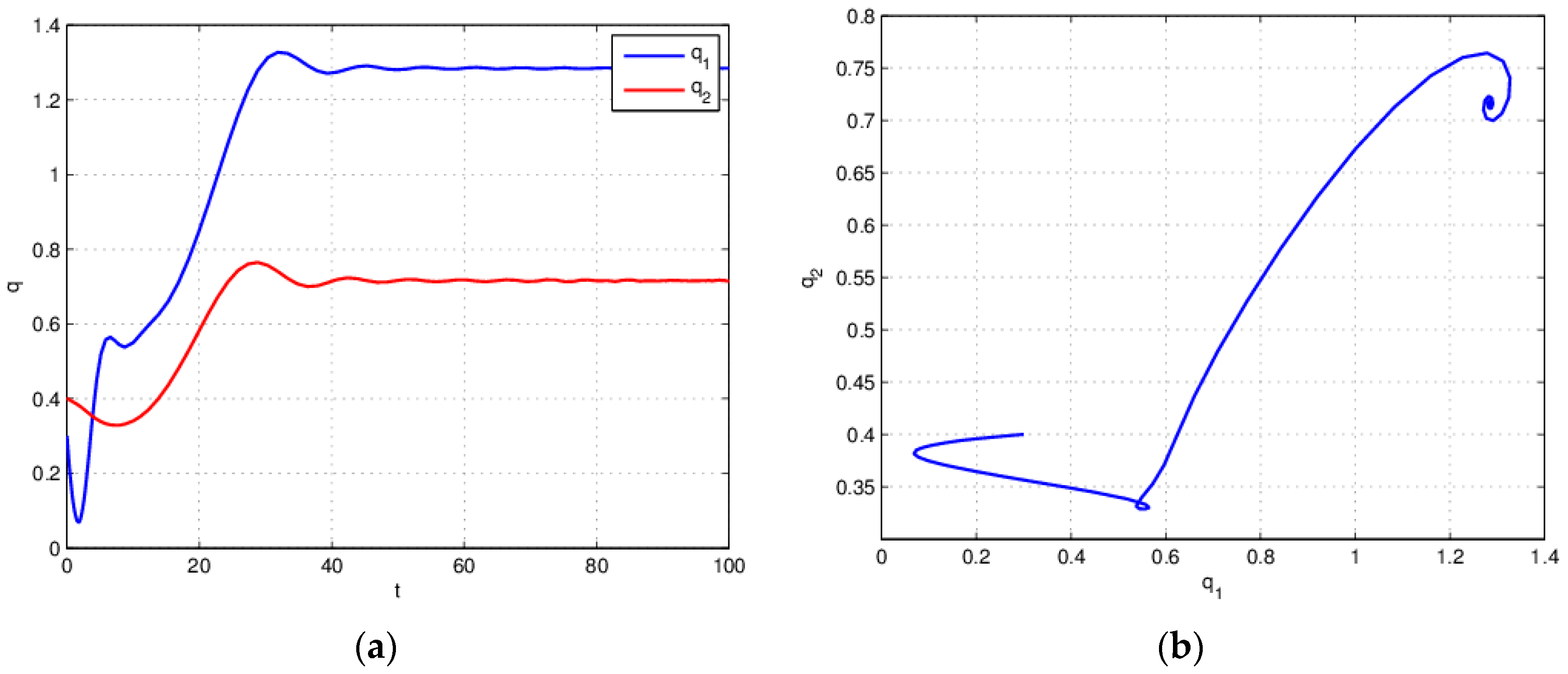
Through the previous analysis, we know that if the parameter values are not reasonable, the system will be instable, even chaotic. A system in a state of chaos will lead to market fluctuations. Therefore, some measures must be taken to maintain the stability of the system. The instable system can be controlled to restore it to a stable state.

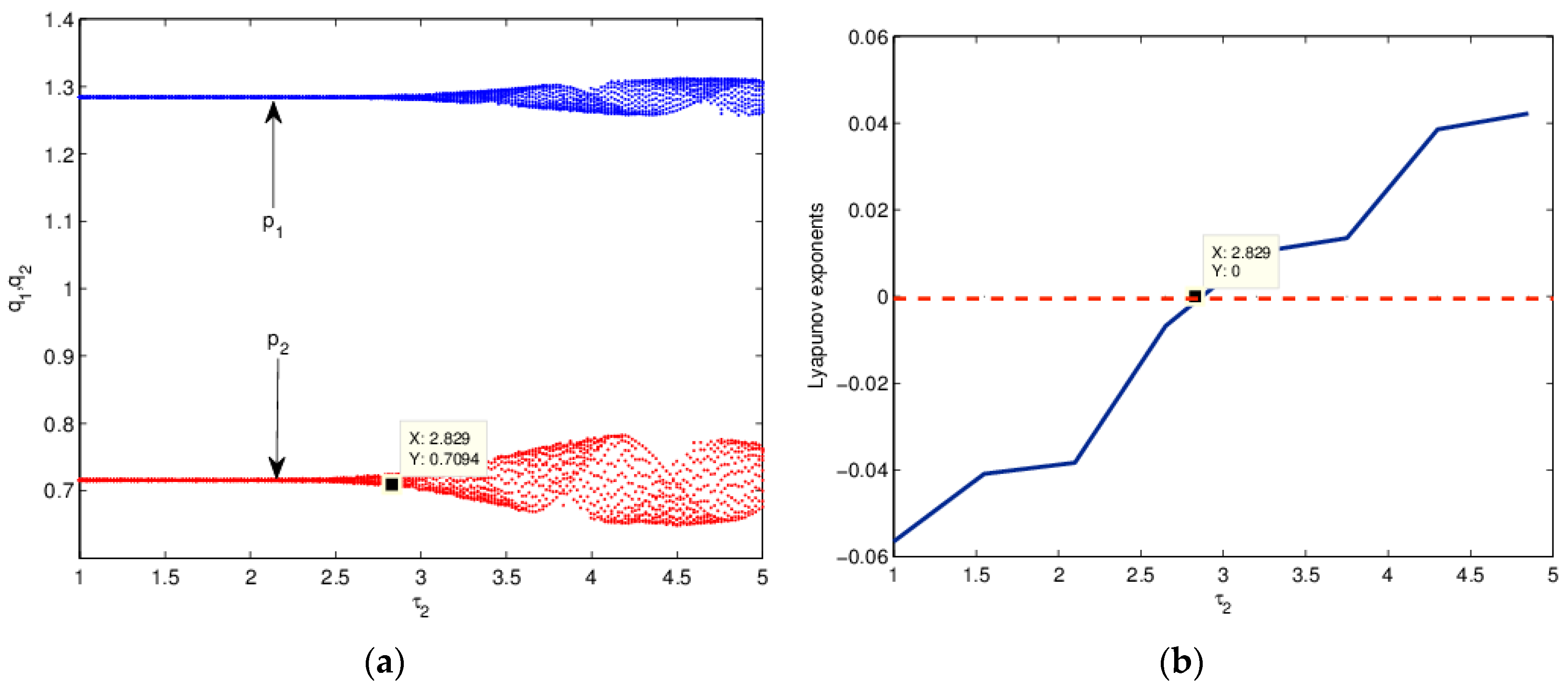
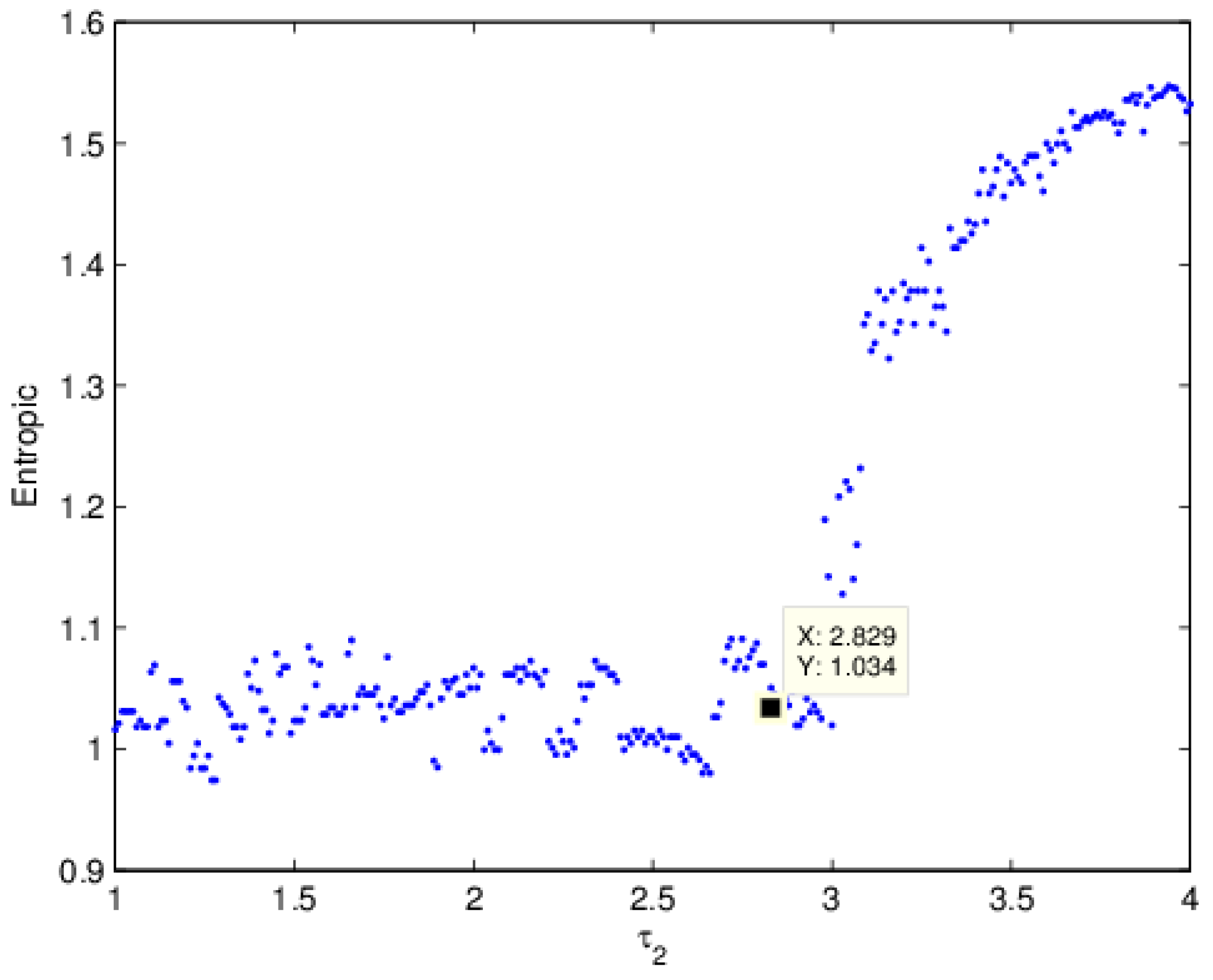
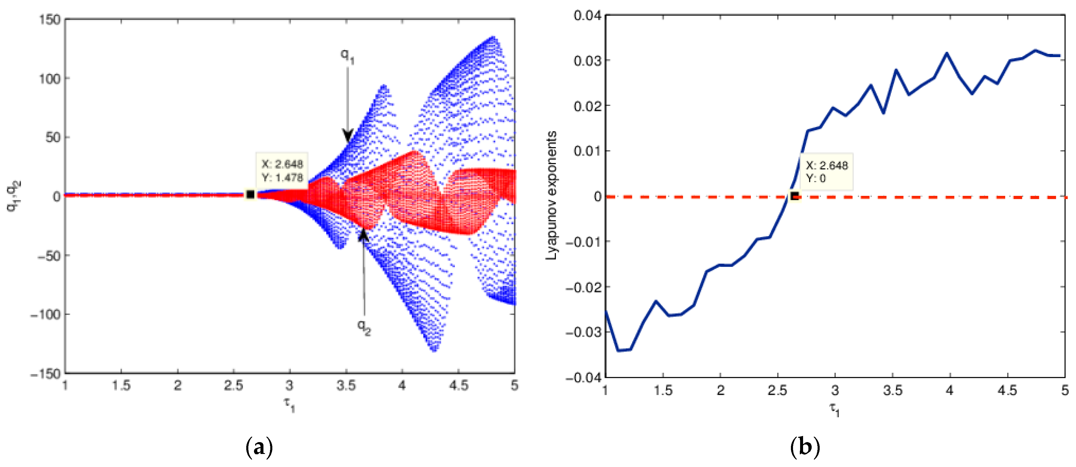
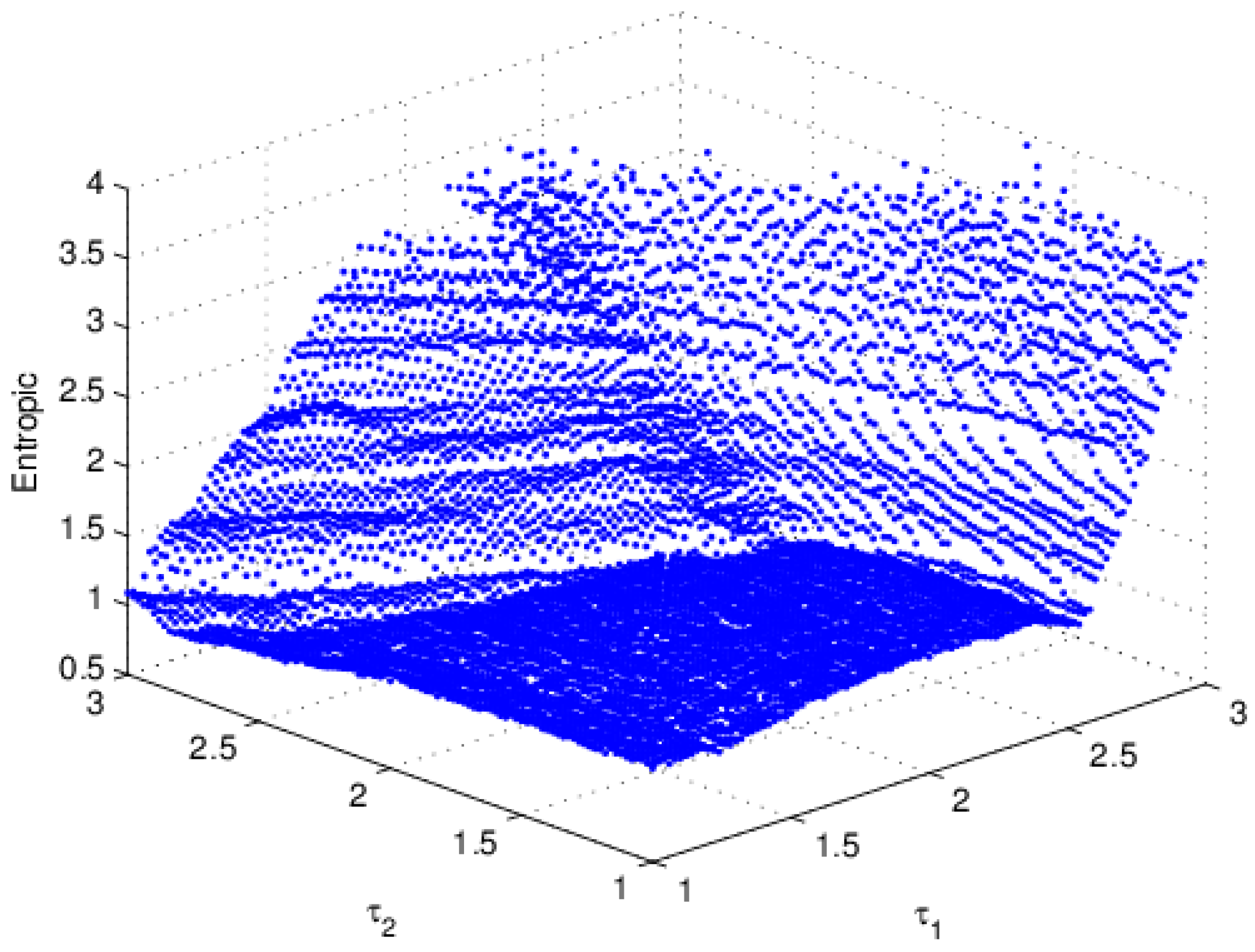
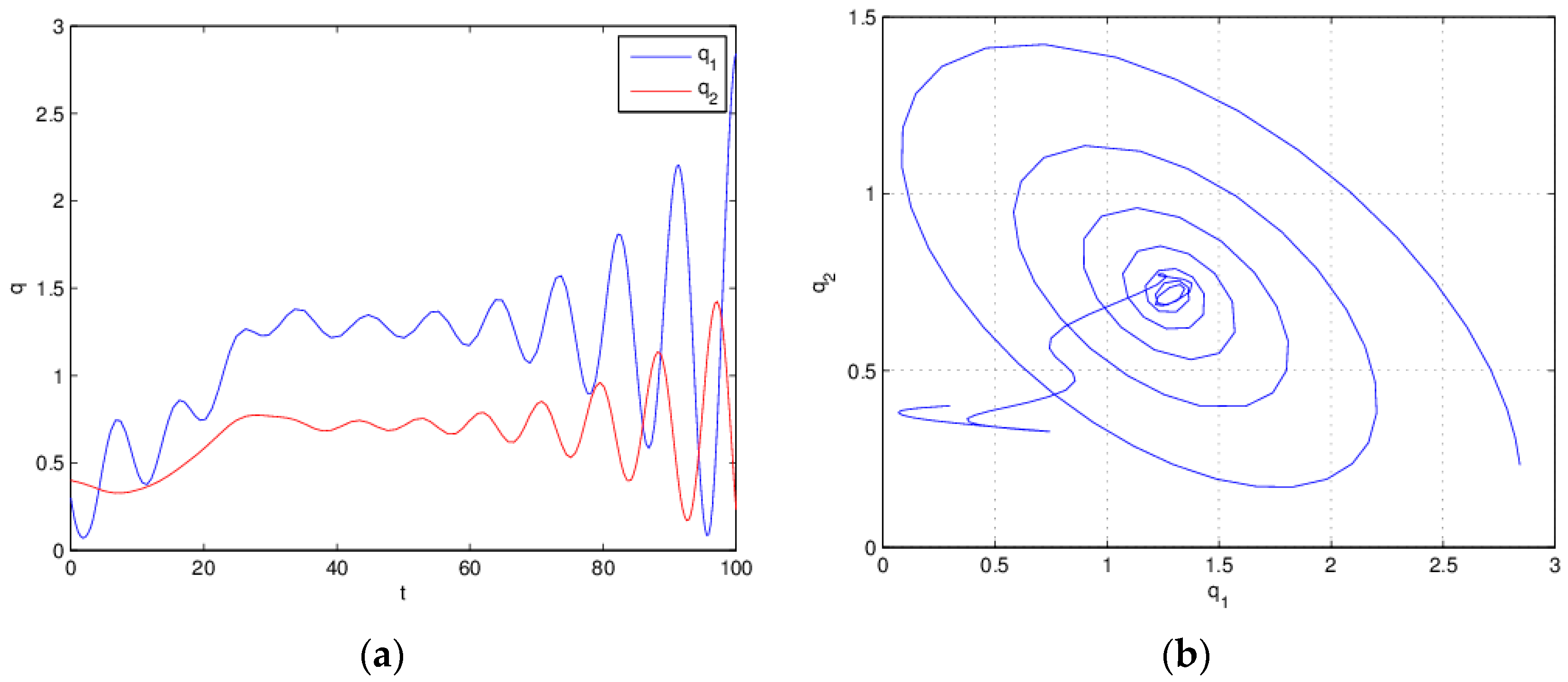
From the analysis in Section 4.2, we know that when ${\tau }_1=3,{\tau }_2=1.5$, the system is chaotic; the effect is shown in Figure 7. From Figure 10 of Section 4.3, ${\tau }_1=3,{\tau }_2=1.5$ is in the blue region; it can be clearly seen that the system is chaotic. We consider the following control system using the delayed feedback control method:

$$\{\begin{array}{l}{\dot{x}}_1=0.05x_1-q_1,\\ {\dot{x}}_2=0.05x_2-q_2,\\ {\dot{q}}_1=(-0.28q_1-0.42q_1(t-{\tau }_1)-0.32x_2+0.21x_1,\\ {\dot{q}}_2=(2.6-0.52q_1-0.78q_1(t-{\tau }_1)-0.78q_2-0.52q_2(t-{\tau }_2))\\ (-0.0084q_2-0.0056q_2(t-{\tau }_2)-0.0064x_1+0.00427x_2)-\mu (q_2-q_2(t-{\tau }_2)).\end{array}.$$

(26)

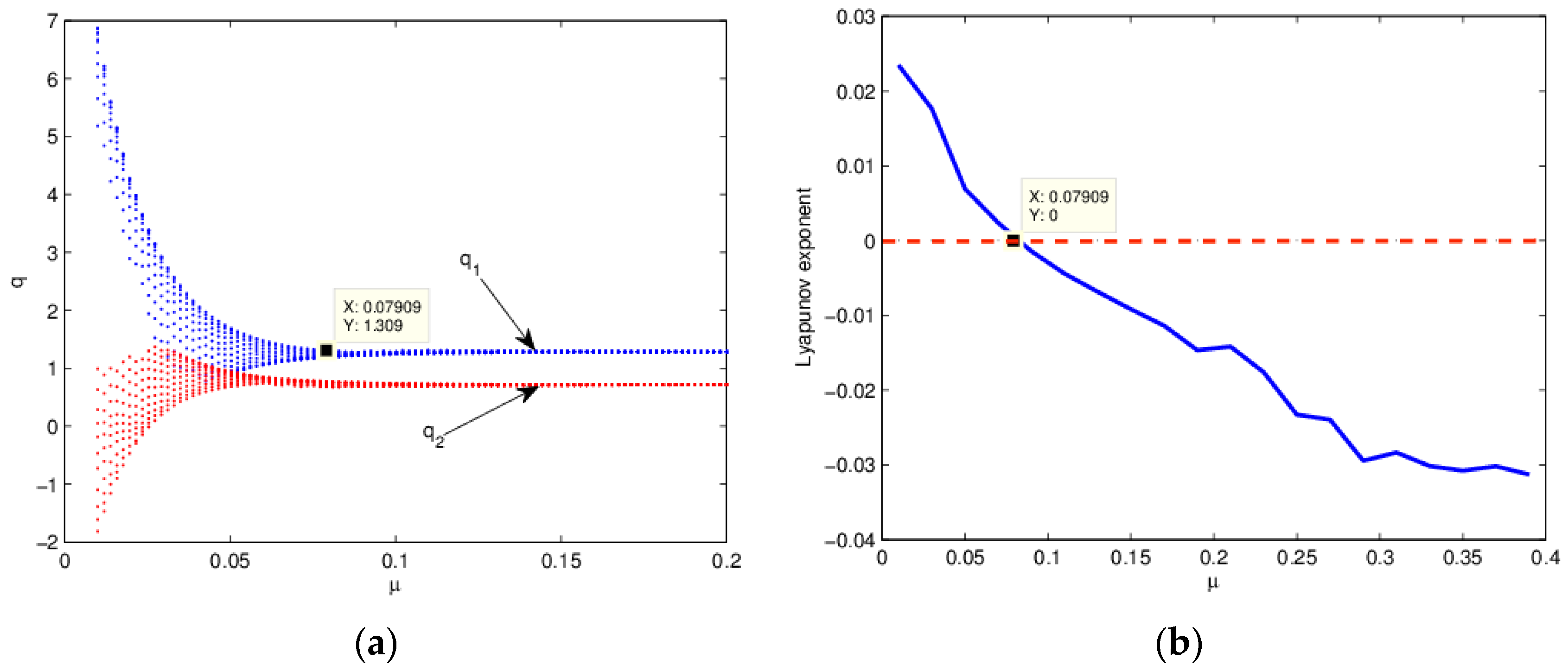
Only adjusting the control parameter $\mu$ while the other parameters are kept constant to realize the control of chaos. Similar to the derivation process in Section 3, the system can obtain bifurcation point $\mu =0.07909$ for ${\tau }_1=3$, ${\tau }_2=1.5$. From Figure 14, we can see that Equation (26) changes from a chaotic state to a steady state as $\mu$ increases. When $\mu =0.07909$, the system undergoes bifurcation. That is to say, when $\mu \in (0,0.07909)$, the system is chaotic; when $\mu \in (0.07909,0.2]$, the system is stable.

Figure 14. The influence of $\mu$ on the stability of Equation (26). (a) Bifurcation diagram; (b) the Largest Lyapunov exponent.

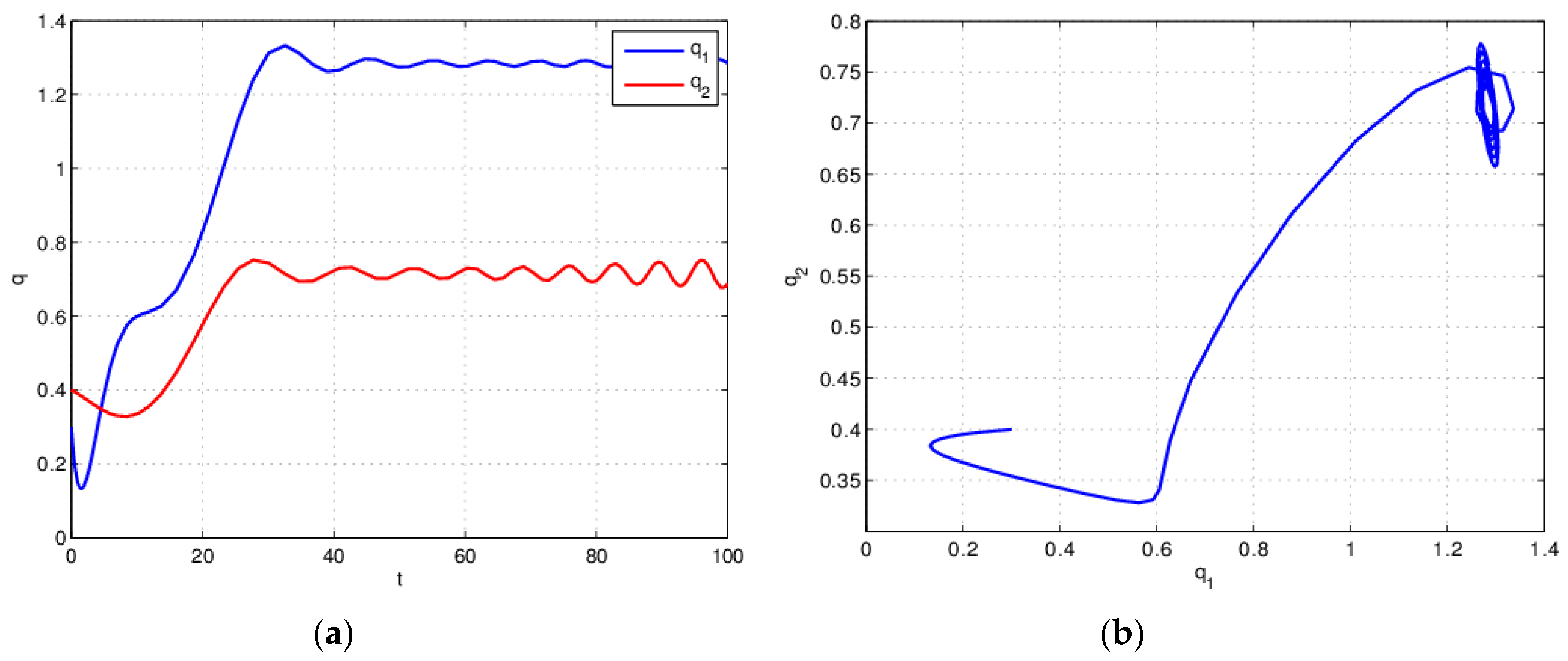
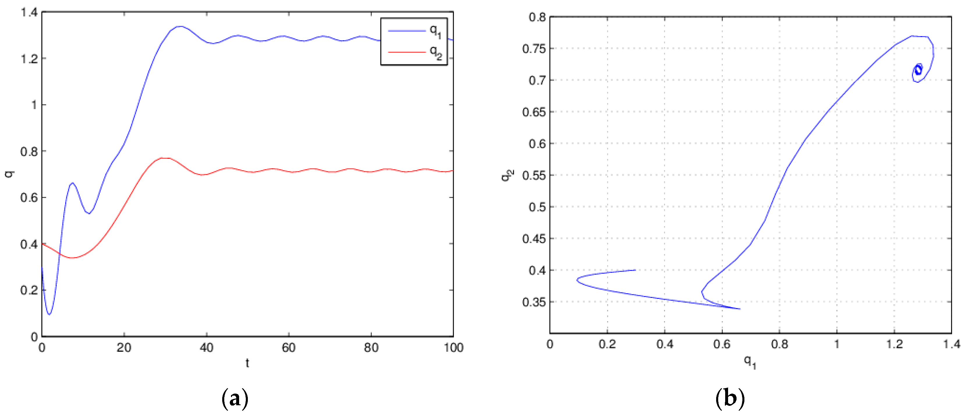
In order to verify the correctness of the above analysis, set $\mu =0.03<0.07909$; according to the analysis, the system should be chaotic at this time. Figure 15 proves the correctness of the conclusion. When we let $\mu =0.15>0.07909$, it can be seen that the system is stable at this time in Figure 16; that is, the chaotic system has been effectively controlled.

Figure 15. Equation (26) is instable when $\mu =0.03<0.07909$ for ${\tau }_1=3,{\tau }_2=1.5$. (a) Time series plot; (b) attractor.

Figure 16. Equation (26) is stable when $\mu =0.15>0.07909$ for ${\tau }_1=3,{\tau }_2=1.5$. (a) Time series plot; (b) attractor.

6. Conclusions

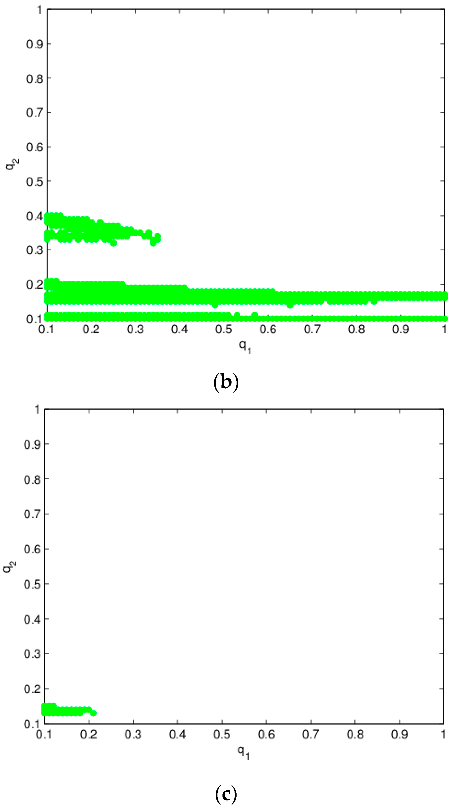
A game model of the duopoly with two delays in the hydropower market is established. The influence of time delay parameters on the stability of the game model is studied. Firstly, the existence and stability of Hopf bifurcation are studied, and the conditions of bifurcation are given. The analysis is carried out in two aspects: ${\tau }_1=0$, ${\tau }_2>0$ and ${\tau }_1>0$, ${\tau }_2>0$. Secondly, the numerical simulation and analysis are carried out on the theoretical derivation. The specific analysis is developed from four aspects: the influence of ${\tau }_2$ on the stability of the system for ${\tau }_1=0$ simulated by using time series, attractor, bifurcation diagram, Lyapunov exponent, and entropic; ${\tau }_2$ fixed, the influence of ${\tau }_1$ on the stability of the system discussed by using time series and basin of attraction; the influence of ${\tau }_1$ and ${\tau }_2$ on the stability of the system displayed by 3D surface chart, 2D parameter bifurcation diagram, and 3D entropic diagram; the influence of ${\tau }_1$, ${\tau }_2$, and ${\mu }_1$ on the stability of the system simulated through a 4D cubic chart and 3D parameter bifurcation diagram. The stability regions of the system are given for each aspect of the specific analysis. The conclusions of the above analysis can provide decision-making guidelines for enterprises to maintain market stability. Finally, the chaotic system is controlled effectively by the method of delayed feedback control, which can efficiently return a chaotic system to a stable state. For future study, we can consider the influence of more factors on the stability of the system, so that it is closer to reality.

References

- Weidou, N.; Johansson, T.B. Energy for Sustainable Development in China. Energy Policy 2004, 32, 1225–1229. [Google Scholar] [CrossRef]
- Nwaobi, G.C. Emission Policies and the Nigerian Economy: Simulations from a Dynamic Applied General Equilibrium Model. Energy Econ. 2004, 26, 921–936. [Google Scholar] [CrossRef]
- Vera, I.; Langlois, L. Energy Indicators for Sustainable Development. Energy 2007, 32, 875–882. [Google Scholar] [CrossRef]
- Omri, A. An international literature survey on energy-economic growth nexus: Evidence from country-specific studies. Renew. Sustain. Energy Rev. 2014, 38, 951–959. [Google Scholar] [CrossRef]
- Dajka, J.; Łobejko, M.; Sładkowski, J. Payoffs and Coherence of a Quantum Two-Player Game in a Thermal Environment. Entropy 2015, 17, 7736–7751. [Google Scholar] [CrossRef]
- Harré, M.S.; Bossomaier, T. Strategic islands in economic games: Isolating economies from better outcomes. Entropy 2014, 16, 5102–5121. [Google Scholar] [CrossRef]
- Ma, J.H.; Ji, W.Z. Complexity of repeated game model in electric power triopoly. Chaos Solitons Fractals 2009, 40, 1735–1740. [Google Scholar] [CrossRef]
- Batabyal, A.A.; Beladi, H. A Stackelberg Game Model of Trade in Renewable Resources with Competitive Sellers. Rev. Int. Econ. 2006, 14, 136–147. [Google Scholar] [CrossRef]
- Sun, Z.H.; Ma, J.H. Complexity of triopoly price game in Chinese cold rolled steel market. Nonlinear Dyn. 2012, 67, 2001–2008. [Google Scholar] [CrossRef]
- Halkos, G.; Papageorgiou, G. Extraction of non-renewable resources: A differential game approach. Arch. Econ. Hist. 2008, 1, 5–22. [Google Scholar]
- Liao, G.C. A novel evolutionary algorithm for dynamic economic dispatch with energy saving and emission reduction in power system integrated wind power. Energy 2011, 36, 1018–1029. [Google Scholar] [CrossRef]
- Yoon, K.H.; Ratti, R.A. Energy price uncertainty, energy intensity and firm investment. Energy Econ. 2011, 33, 67–78. [Google Scholar] [CrossRef]
- Chang-Jian, C.W.; Chang, S.M. Bifurcation and chaos analysis of spur gear pair with and without nonlinear suspension. Nonlinear Anal. Real World Appl. 2011, 12, 979–989. [Google Scholar] [CrossRef]
- Lü, J.H.; Chen, G.; Celikovský, S. Bridge the gap between the Lorenz system and the Chen system. Int. J. Bifurc. Chaos 2002, 12, 2917–2926. [Google Scholar] [CrossRef]
- Celikovský, S.; Chen, G. On a generalized Lorenz canonical form of chaotic systems. Int. J. Bifurc. Chaos 2002, 12, 1789–1812. [Google Scholar] [CrossRef]
- Sun, M.; Tian, L.X.; Fu, Y.; Qian, W. Dynamics and adaptive synchronization of the energy resource system. Chaos Solitons Fractals 2007, 31, 879–888. [Google Scholar] [CrossRef]
- Sun, M.; Tian, L.X.; Zeng, C.Y. The energy resources system with parametric perturbations and its hyperchaos control. Nonlinear Anal. Real World Appl. 2009, 10, 2620–2626. [Google Scholar] [CrossRef]
- Sun, M.; Wang, X.F.; Chen, Y.; Tian, L.X. Energy resources demand-supply system analysis and empirical research based on non-linear approach. Energy 2011, 36, 5460–5465. [Google Scholar] [CrossRef]
- Hassard, B.D.; Kazarinoff, N.D.; Wan, Y.H. Theory and Applications of Hopf Bifurcation; Cambridge University Press: Cambridge, UK, 1981. [Google Scholar]
© 2016 by the authors; licensee MDPI, Basel, Switzerland. This article is an open access article distributed under the terms and conditions of the Creative Commons Attribution (CC-BY) license (http://creativecommons.org/licenses/by/4.0/).