Abstract
Multiscale entropy (MSE) quantifies the cardiovascular complexity evaluating Sample Entropy (SampEn) on coarse-grained series at increasing scales τ. Two approaches exist, one using a fixed tolerance r at all scales (MSEFT), the other a varying tolerance r(τ) adjusted following the standard-deviation changes after coarse graining (MSEVT). The aim of this study is to clarify how the choice between MSEFT and MSEVT influences quantification and interpretation of cardiovascular MSE, and whether it affects some signals more than others. To achieve this aim, we considered 2-h long beat-by-beat recordings of inter-beat intervals and of systolic and diastolic blood pressures in male (N = 42) and female (N = 42) healthy volunteers. We compared MSE estimated with fixed and varying tolerances, and evaluated whether the choice between MSEFT and MSEVT estimators influence quantification and interpretation of sex-related differences. We found substantial discrepancies between MSEFT and MSEVT results, related to the degree of correlation among samples and more important for heart rate than for blood pressure; moreover the choice between MSEFT and MSEVT may influence the interpretation of gender differences for MSE of heart rate. We conclude that studies on cardiovascular complexity should carefully choose between fixed- or varying-tolerance estimators, particularly when evaluating MSE of heart rate.
1. Introduction
A feature of heart rate variability, potentially useful for improving the stratification of cardiovascular risk or for detecting early alterations of the cardiovascular control, is the level of unpredictability of beat-by-beat dynamics. One of the most popular estimators of heart-rate unpredictability is Sample Entropy (SampEn) [1], proposed as an unbiased variant of Approximate Entropy (ApEn) [2]. SampEn is based on the calculation of the conditional probability that any two segments of m beats that are similar remain similar when their length increases by one beat. In the estimation of SampEn or ApEn, each segment is represented as a point in an m-dimensional space and two segments are similar if their distance is lower than a given tolerance, r. The tolerance r is a fraction, ρ, of the standard deviation, SD, of the series (r = ρ × SD) with ρ typically ranging between 10% and 25% [2].
Heart rate variability reflects part of the overall complexity of cardiovascular control. The latter regulates the amount of blood flow received by individual vascular beds, which compose a fractal network of vessels, each with its own time-varying local needs. For this reason, some authors hypothesized that multiscale analyses better describe the cardiovascular complexity and proposed a multiscale estimator of entropy [3]. Their approach is based on the evaluation of SampEn on coarse-grained heart-rate series with coarse-graining order τ, in number of beats, progressively increasing from τ = 1. The tolerance r is calculated as fraction of the SD of the original series, and the same r is used for evaluating SampEn at all scales τ greater than 1.
However, this approach is matter of discussion because coarse graining changes SD, which therefore is function of the coarse graining order: SD(τ) [4]. It has been argued that if the same r is used at all the scales, SampEn incorrectly estimates entropy because the wrong threshold is used for τ > 1. Alternatively, a tolerance varying with τ: r(τ) = ρ × SD(τ) has been proposed. This criticism was rejected by the authors of the original proposal, who explained that SD changes due to coarse graining “are related to the temporal structure of the original time series, and should be accounted for” in the evaluation of multiscale entropy [5]. This debate did not clarify the issue sufficiently well and, at present, two theoretically different approaches are used for evaluating multiscale entropy (MSE). One approach, MSEFT, is based on the use of a fixed tolerance r, fraction of SD of the original series, for all the scales. The other approach, MSEVT, is based on the use of a varying tolerance r(τ), adjusted at each scale τ as fraction of the SD of the coarse-grained series.
This methodological aspect appears to have been overlooked in the literature. Often MSE estimates of heart rate variability do not explicitly indicate whether they used a fixed or a varying tolerance. Furthermore, to our knowledge, only a couple of studies directly compared the two approaches. These studies showed that MSEFT and MSEVT changed similarly in congestive heart failure patients [6] or in a rat model of hypertension and congestive heart failure [7], suggesting that at least in this clinical setting and animal model, the methodological difference is not relevant. However, the real influence of the choice between fixed and varying tolerance on MSE in healthy humans or in other classes of patients remains unknown, and it is also unclear whether possible differences between the two approaches affect MSE of heart rate and of other cardiovascular series differently.
It should be considered that this methodological issue is more general than it may appear. In fact, it regards not only the MSE algorithm as originally proposed in [3], but also successive variants based on SampEn, as Composite [8] and Refined-Composite MSE [9], Short-Time MSE [10], Modified MSE [11] and Refined MSE [12], as well as fuzzy MSE [13], being all these methods based on the definition of a tolerance that can be or not be adapted to the SD changes associated with coarse graining.
Therefore, the aim of this study is to evaluate how the choice between fixed and varying tolerances among scales actually (1) influence the estimation of MSE in healthy individuals; (2) concern some cardiovascular signals more than other; and (3) may affect the physiological interpretation of the results. For this aim, we compared MSEFT and MSEVT in male and female groups of healthy volunteers, considering cardiovascular series often recorded in physiological and clinical studies: inter-beat interval (IBI, the inverse of heart rate); systolic blood pressure (SBP) and diastolic blood pressure (DBP); and we evaluated how the choice between fixed- and varying-tolerance affects the interpretation of MSE comparisons by gender.
2. Materials and Methods
2.1. Subjects and Data Collection
We considered a subset of the continuous beat-by-beat recordings of blood pressure obtained in two previous studies aimed at evaluating the effects of dietary salt on the cardiovascular regulation in normotensive volunteers [14] and in hypertensive individuals with a never-treated mild or moderate uncomplicated essential hypertension [15]. From our database, we selected recordings of 42 female and 42 male participants matched by prevalence of hypertension (38.1% in both groups), age (34.3 ± 9.7 years in females, 34.4 ± 10.1 years in males, mean ± SD) and body mass index (22.6 ± 2.8 kg/m2 in females, 23.6 ± 2.4 kg/m2 in males). Participants had neither history nor physical or laboratory evidence of cardiovascular disease. They were studied after a low-salt diet (30 mmol NaCl per day) of 5 days, to minimize the confounding effects of sodium on cardiovascular variability. Data were collected in the morning, sitting in a quite environment. Arterial blood pressure was recorded for 2 h at the finger artery level by Portapres (Finapres Medical Systems B.V., Amsterdam, The Netherlands) deriving SBP, DBP and IBI (as time interval between SBP values) beat by beat.
2.2. Synthesized Time Series
Synthesized time series were used to test the performances of MSEFT and MSEVT estimators. The dsp.ColoredNoise (Version 9.1) routine in Matlab (R2015b) generated white noise, “1/f” noise and brown noise series of N = 8400 samples to simulate the length of cardiovascular series of 2-h duration at the average heart rate of 70 bpm. For each type of noise, 100 time series were generated.
2.3. MSE Estimators
Given a series of N beats, {x(j)} with 1 ≤ j ≤ N, we obtained the standardized series {x′(j)}, with zero mean and unit variance, as
with σ and μ standard deviation and mean of {x(j)}. Coarse-grained series of order τ for 1 ≤ τ ≤ 30 and 1 ≤ i ≤ int (N/τ) were derived as:
x′(j) = (x(j) − μ)/σ
Setting the maximum coarse graining order at τ = 30 we obtained series with length of at least 280 samples for 2-h recordings at the average heart rate of 70 bpm. The pedix “L” in (2) indicates that the coarse graining covers the series starting from the left side, i.e., from j = 1. Let’s call SDL(τ) the standard deviation of {yLτ(i)}. Because of the normalization in Equation (1), SDL(1) = 1. Multiscale entropy with fixed tolerance, MSELFT (τ,m), was evaluated as in [3], but extending the range of scales up to τ = 30 (see Appendix A) and the embedding dimension m between 1 and 3. In this study, we set ρ = 20% and thus r = 0.20.
If the length of the time series is not multiple of the coarse graining order, that is, if q = τ mod N is greater than 0, then the last data segment of q samples does not contribute to coarse graining. To also take into account the last q data, a “right-sided” coarse graining was performed:
The pedix “R” in (3) indicates that the coarse graining covers the series up to the right side, i.e., from j = q + 1 up to j = N. Multiscale entropy, MSERFT (τ,m), was calculated similarly for {yRτ(i)}. The final estimate was the average of left- and right-sided estimates:
MSEFT (τ,m) = ½ × [MSERFT (τ,m) + MSELFT (τ,m)]
Following Equation (4), multiscale entropy was also calculated separately for left-sided, MSELVT (τ,m), and right-sided, MSERVT (τ,m), coarse-grained series, with tolerance r(τ) respectively equal to ρ × SDL(τ) or ρ × SDR(τ) and ρ = 20%. The final estimate was the average of left- and right-sided estimates:
MSEVT (τ,m) = ½ × [MSERVT (τ,m) + MSELVT (τ,m)]
The MSEFT and MSEVT estimators were implemented in Matlab making use of the sampen.m code available on the physionet website [16].
2.4. Statistical Analysis
Multiscale entropies of males and females were compared by the unpaired Mann Whitney U test, a nonparametric test that allows making no assumptions on the MSE distributions at any scale τ. The threshold for statistical significance was set at α = 0.05, performing the analysis with “R: A Language and Environment for Statistical Computing” software package (R Core Team, R Foundation for Statistical Computing, Vienna, Austria, 2017).
3. Results
3.1. Synthesized Time Series
Figure 1 compares MSEFT and MSEVT estimates for the synthesized series at m = 2 (the embedding dimension more often used in heart rate variability studies). White noise has the highest entropy and brown noise the lowest entropy at scale τ = 1. At τ > 1, important differences appear between MSEFT and MSEVT for white noise: MSEVT is constant over all the scales while MSEFT decreases quickly with τ. As to “1/f” noise, differences are less marked, but while MSEVT increases with τ, MSEFT converges to a lower constant value. MSEFT and MSEVT of Brown noise are the same and increase with τ.
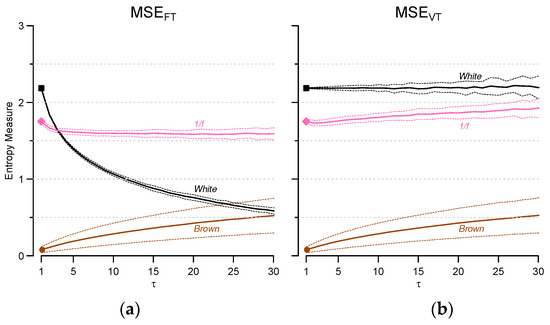
Figure 1.
Multiscale entropy (MSE) estimated for m = 2 with fixed- (a) and varying- tolerance (b) for white noise, “1/f” noise and brownian motion: mean ± SD. Results from 100 series generated for each type of noise (see methods). Note that MSEFT and MSEVT coincide at τ = 1.
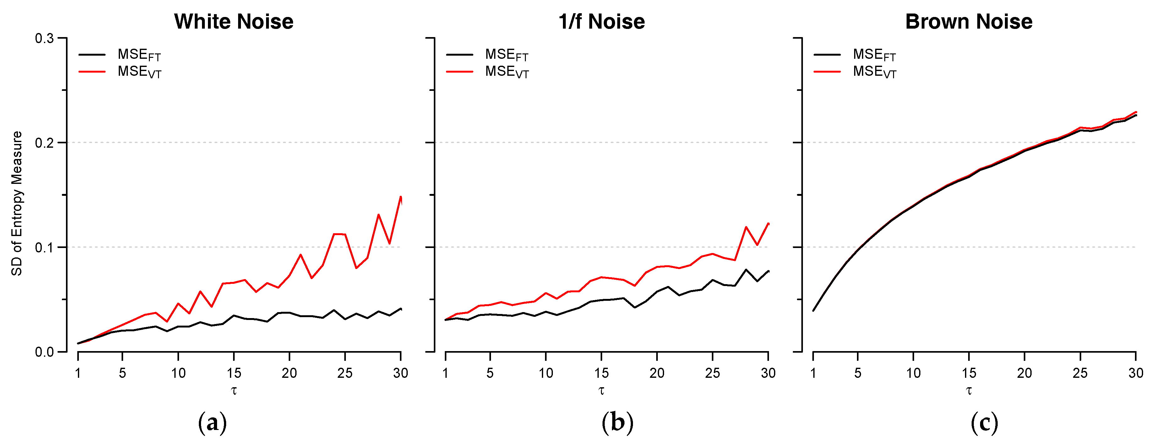
The type of estimator also influences the variability of the estimates, at least for white and “1/f” noise, and the standard deviation of the estimates is lower for MSEFT at all scales (Figure 2).
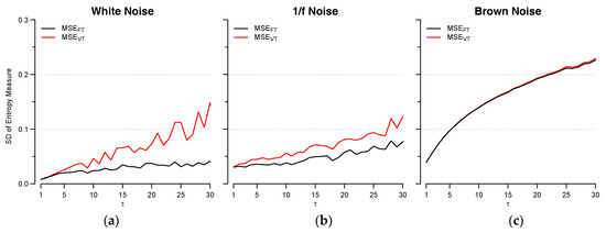
Figure 2.
Standard Deviation of MSEFT (black) and MSEVT (red) estimates for white noise (a); “1/f” noise (b) and brown noise (c). Results from the same synthesized series of Figure 1.
3.2. Cardiovascular Signals
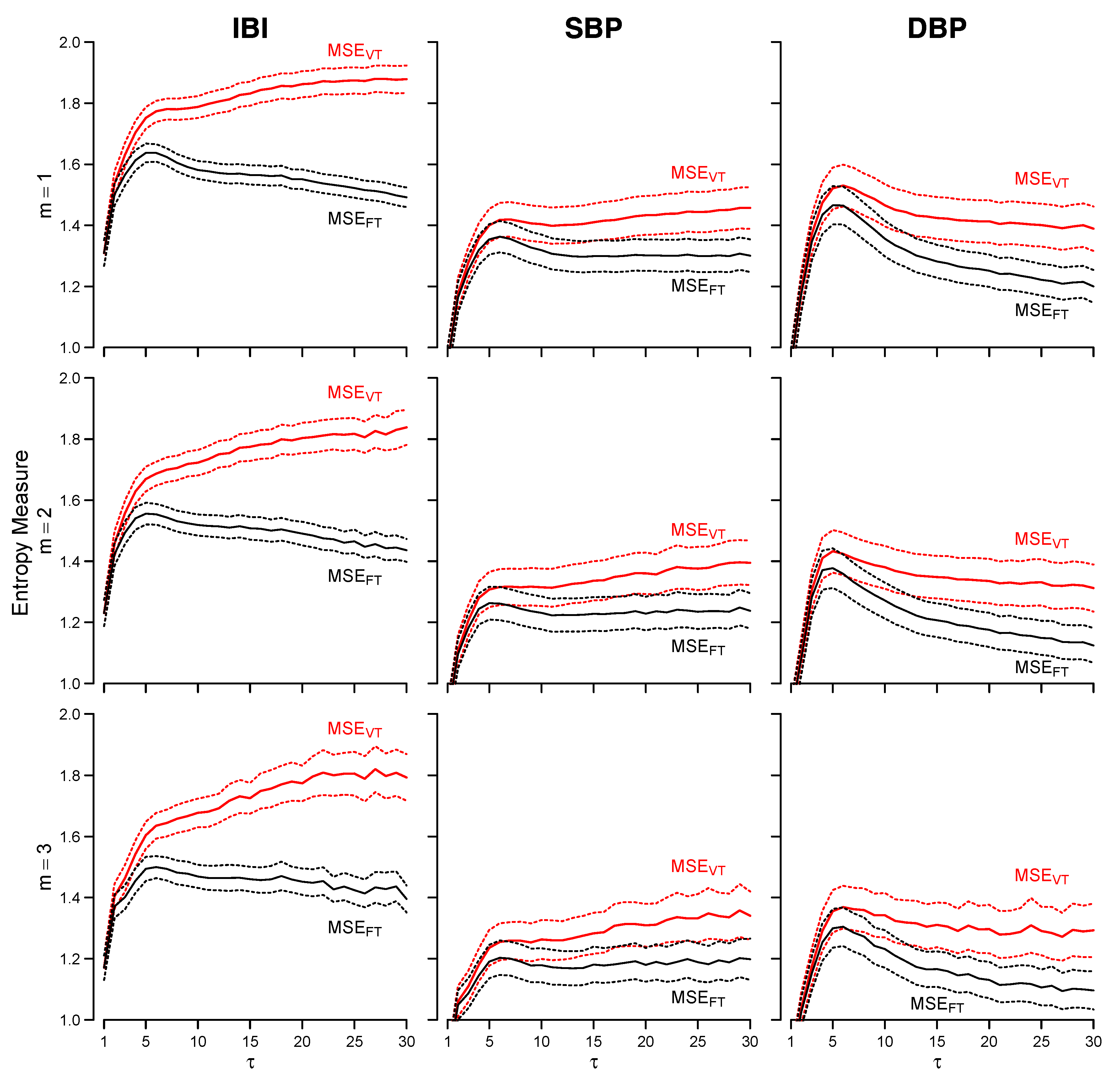
Figure 3 compares MSEFT and MSEVT for IBI, SBP and DBP. The largest discrepancies between MSEFT and MSEVT occur for IBI. MSEFT reaches its maximum at τ = 5, and decreases almost linearly at larger scales. By contrast, MSEVT monotonically increases with the scale and the maximum occurs at τ = 30. Discrepancies between MSEFT and MSEVT are less marked for SBP, but also in this case the highest entropy is reached at τ = 5 for MSEFT and at τ = 30 for MSEVT. The two estimators provide similar trends for DBP, with maximum at τ = 5. However, like for IBI and SBP, the MSEFT and MSEVT estimators diverge at the larger scales also for DBP.
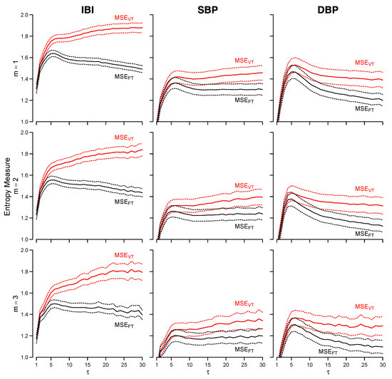
Figure 3.
MSEVT (red lines) and MSEFT (black lines) for inter-beat interval (IBI), systolic blood pressure (SBP) and diastolic blood pressure (DBP) series, and embedding dimensions m from 1 to 3. Mean ± 95% confidence intervals of the mean over the group (N = 84).
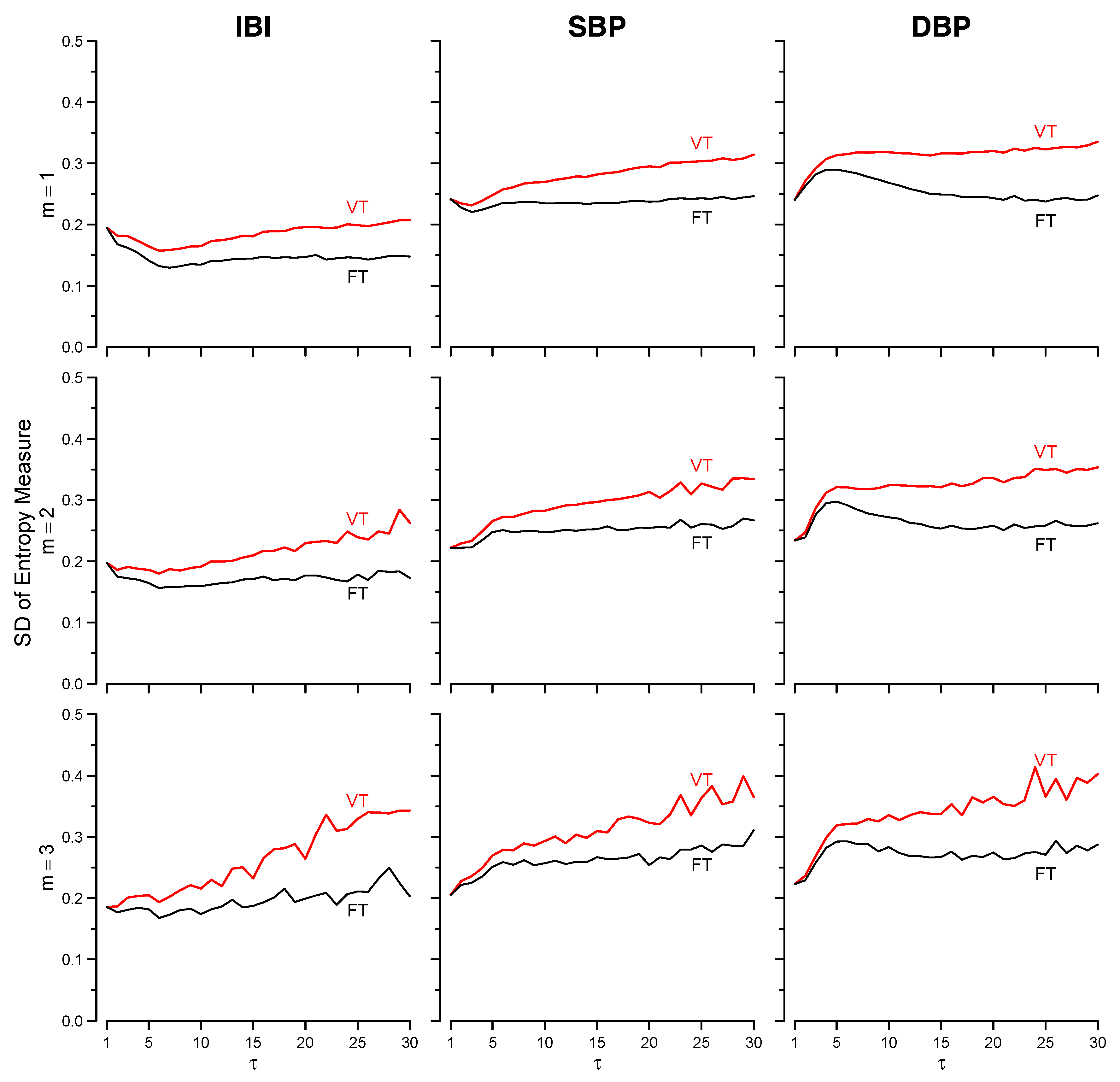
The estimator precision is greater for MSEFT because the standard deviation over the group of estimates is always lower for MSEFT than for MSEVT (Figure 4). Overall, results do not depend on the embedding dimension, but estimates appear more stable when m = 1 (Figure 3). Therefore, for concision sake, in the following only estimates for m = 1 are presented.
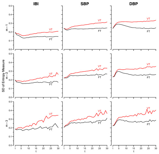
Figure 4.
Standard deviations of MSEVT (red) and MSEFT (black) estimates over the same group of volunteers of Figure 3.
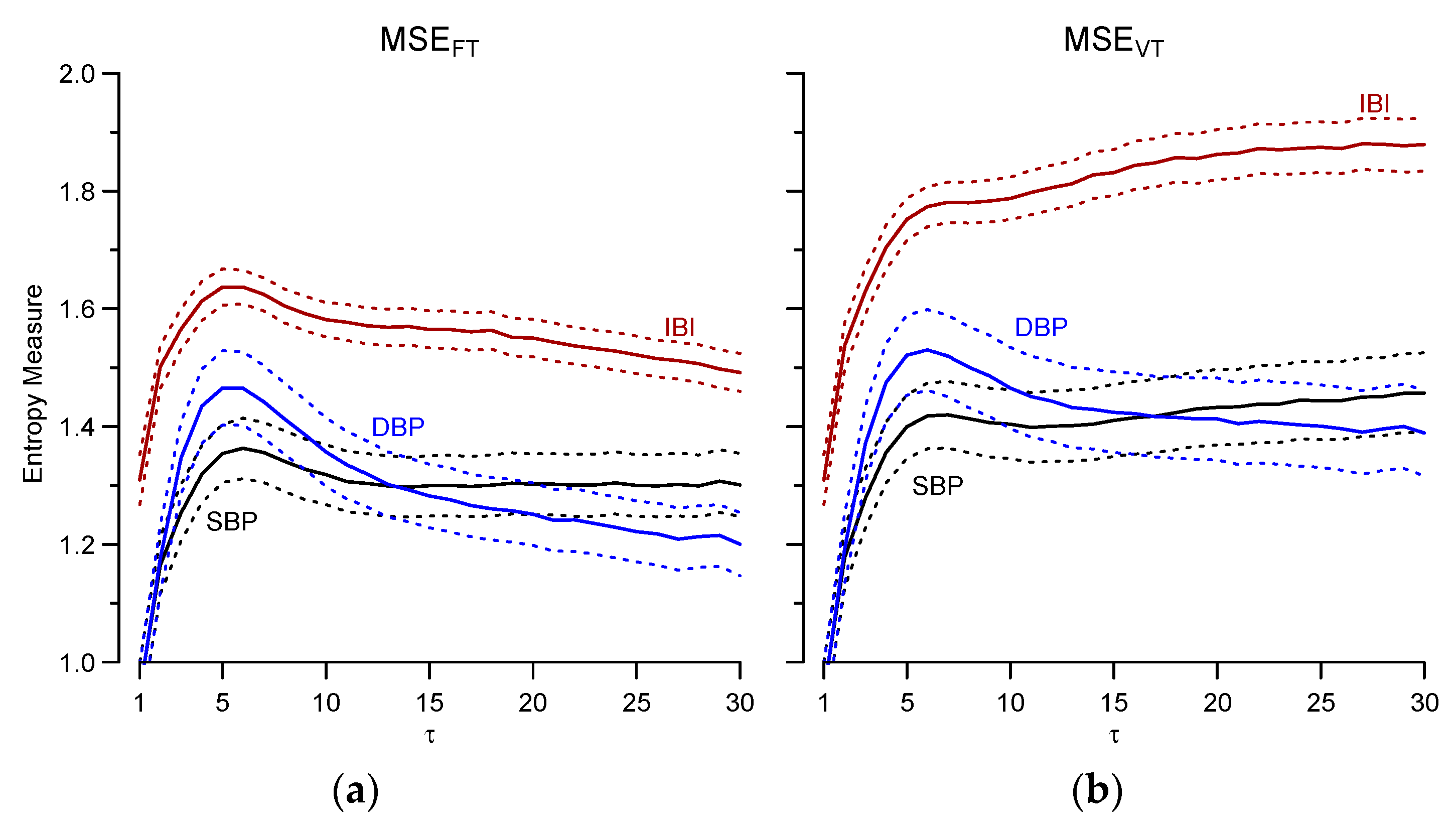
The choice between MSEFT and MSEVT also influences the relative level of entropy among signals (Figure 5). Entropy is higher for IBI than for SBP but while MSEFT estimates converge to similar values at the larger scales, MSEVT estimates do not converge because IBI and SBP entropies increase in parallel with τ. DBP entropy is higher than SBP entropy at the shorter scales, and lower than SBP entropy at the larger scales, but the crossing point occurs at τ < 15 for MSEFT, and at τ > 15 for MSEVT.
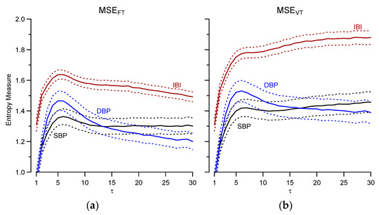
Figure 5.
Comparison among signals of MSEFT (a) and MSEFT (b). Mean ± 95% confidence intervals over the group (N = 84) for m = 1.
3.3. Gender Comparison
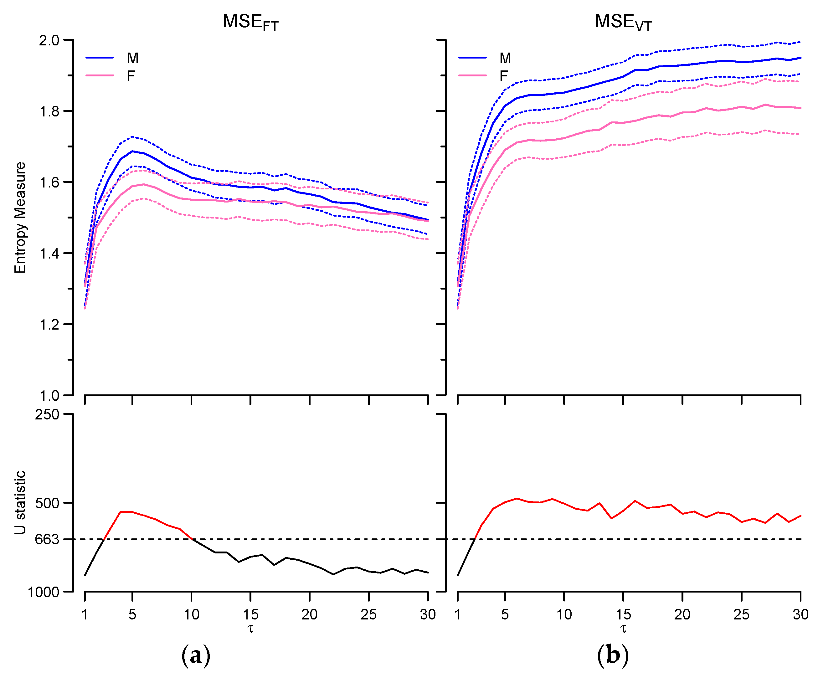
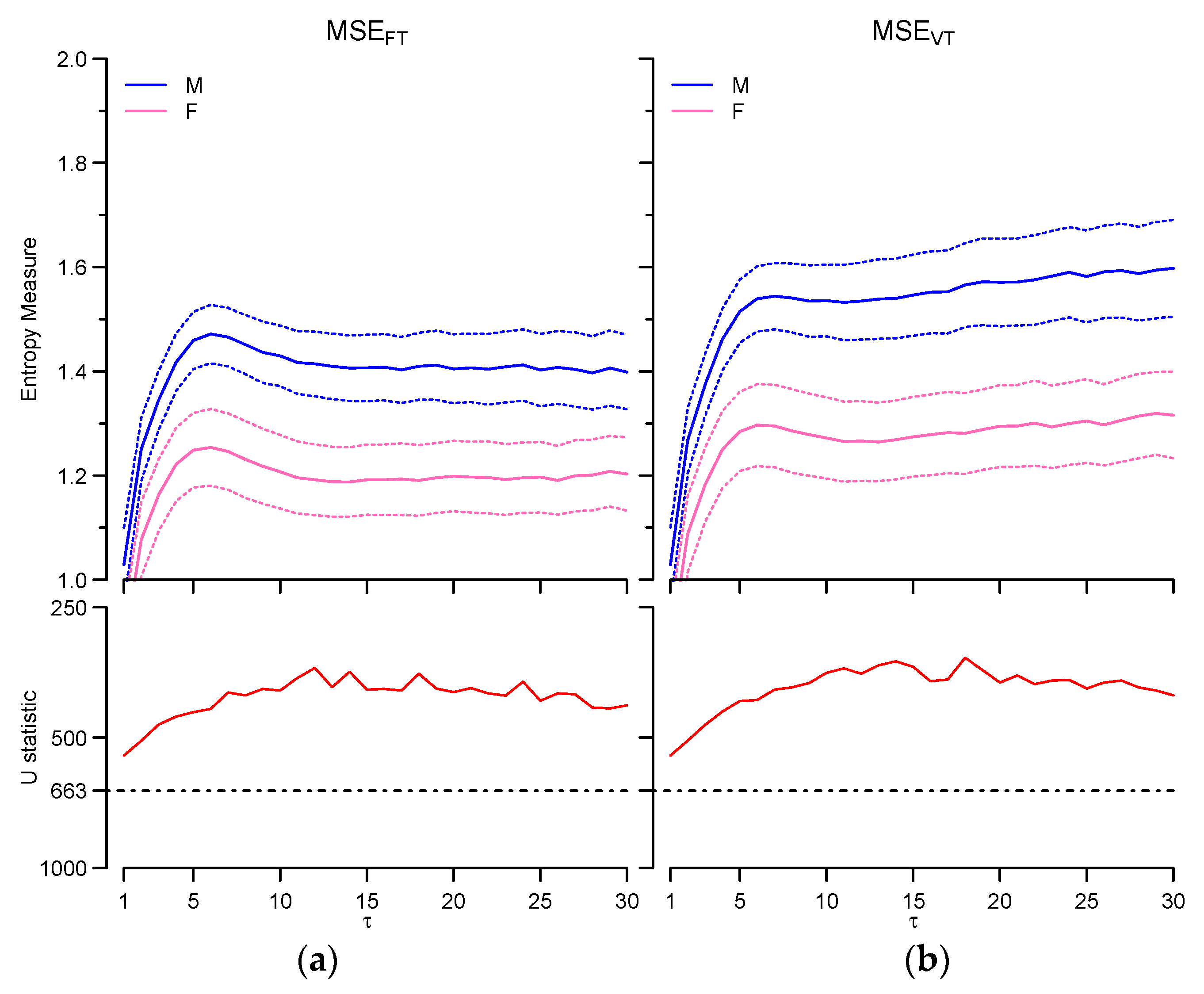
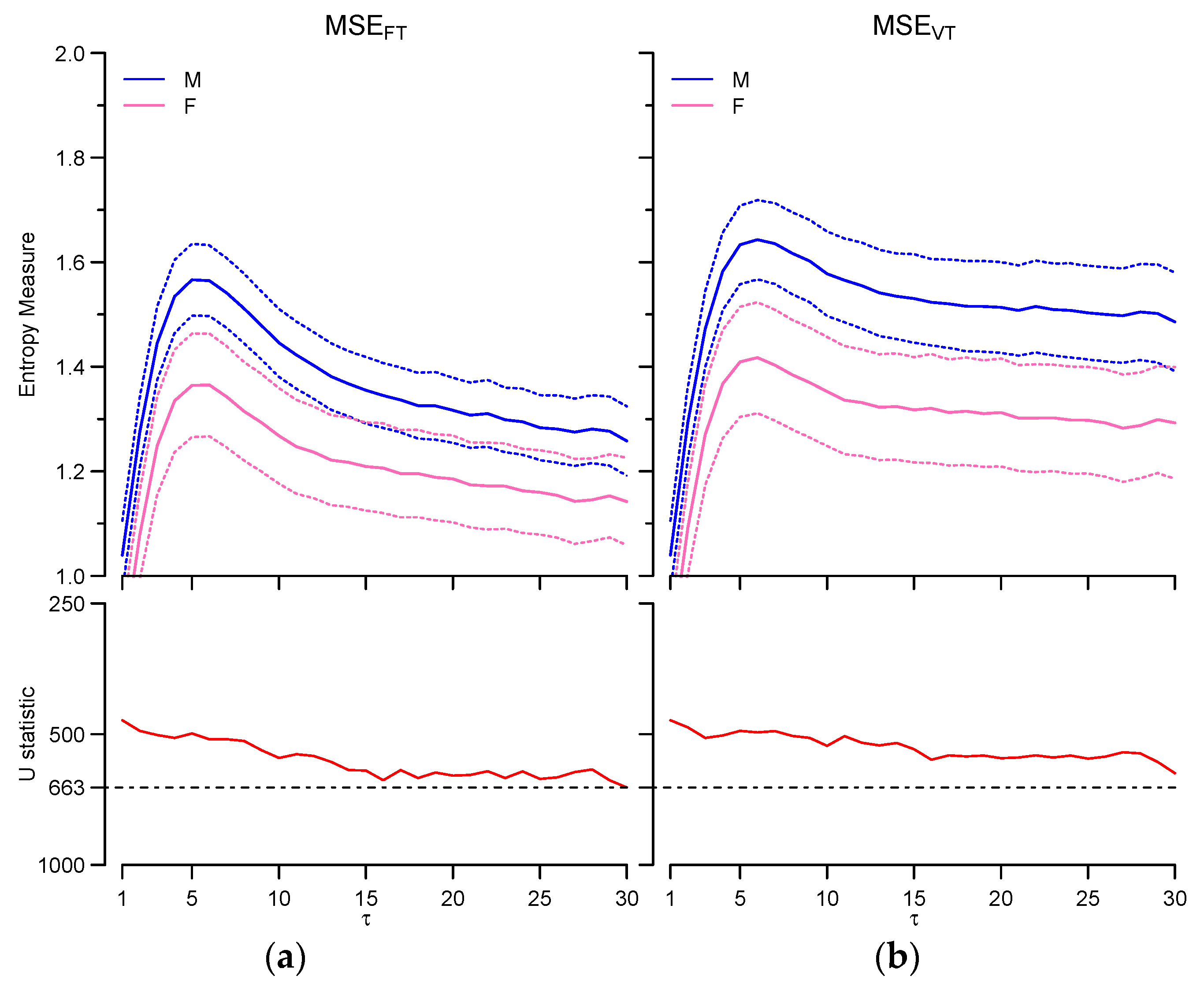
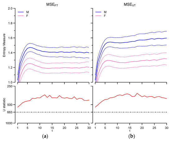
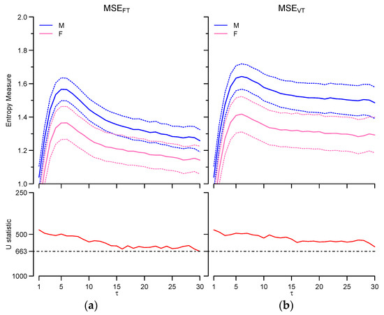
The choice between fixed and varying tolerance influences the scales where gender effects are identifiable, and has a different impact on IBI than on SBP and DBP. If IBI is considered, MSEFT detects a significant effect between τ = 3 and τ = 10 only while MSEVT points out significant differences at all scales ≥3 (Figure 6). The two estimators provide univocal results for blood pressure, and multiscale entropy is greater in males at all the scales for SBP (Figure 7) and DBP (Figure 8).
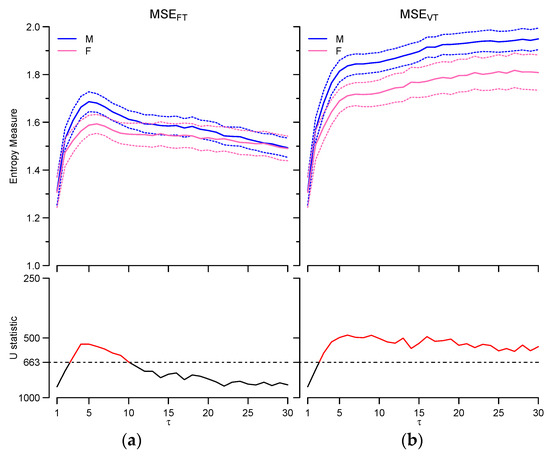
Figure 6.
IBI multiscale entropy: comparison between males (M, N = 42) and females (F, N = 42). Upper panels: MSEFT (a) and MSEVT (b) mean and 95% confidence interval for m = 1. Lower panels: Mann-Whitney U statistics for males vs. females at each τ; the dashed line is the 5% threshold of statistical significance; U values above the threshold (in red) indicate significant differences.
4. Discussion and Conclusions
This work demonstrates that in healthy individuals the choice between a fixed-tolerance and a varying-tolerance approach may substantially influence the estimates of multiscale entropy of cardiovascular time series, and that this choice affects heart rate variability more than blood pressure variability. The analysis of synthesized signals with different correlation properties helps to understand why results by MSEFT and MSEVT differ so importantly.
It has been already demonstrated that SampEn of a sequence of random numbers decreases quickly when ρ (the fraction of SD that defines the tolerance r) increases [1]. Because of SD(τ) changes, the fixed-tolerance approach actually changes ρ to maintain r constant at each coarse graining level τ. Therefore, if ρ of MSEFT increases because SD(τ) decreases with τ, while ρ of MSEVT does not change, we may expect lower entropy estimates by MSEFT than by MSEVT at τ > 1. The way SD(τ) changes with τ depends on the correlation among samples. If {x(j)} is generated by a stationary process with autocorrelation function γ(k), then SD(τ), after standardization and coarse graining of {x(j)} as in Equation (2), is [17]:
If {x(j)} is white noise, γ(k) = 0 for k ≥ 1 and SD(τ) decreases proportionally to τ1/2; if {x(j)} is a “long-memory” process with γ(k) > 0, SD(τ) decreases less steeply with τ. Therefore, for these stochastic processes, the fixed r of MSEFT, which is equal to ρ × SD(1), is greater than r(τ) = ρ × SD(τ), at all scales τ > 1. Moreover, at any τ > 1 the difference between the fixed tolerance of MSEFT and the varying tolerance of MSEVT, r − r(τ), decreases when the correlation among samples increases.
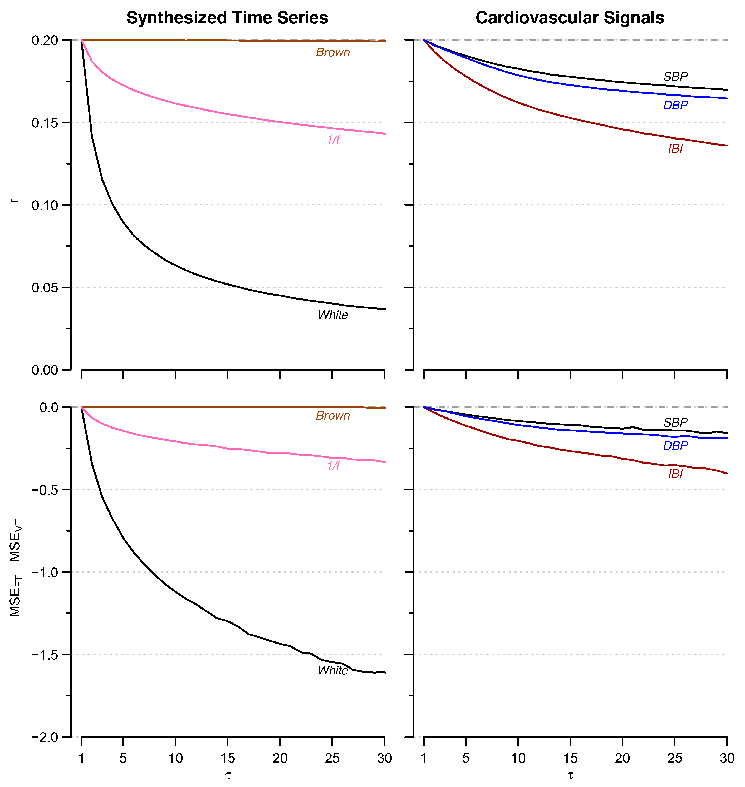
The series synthesized by running the dsp.ColoredNoise routine actually show this trend (see Figure 9, upper left panel), being the discrepancies between fixed and varying thresholds larger for white noise than for “1/f” noise, and null for Brown noise. This explains why MSEFT and MSEVT differ substantially for white noise, differ only slightly for “1/f” noise, and coincide for Brown noise (Figure 1 and Figure 9, lower left panel).
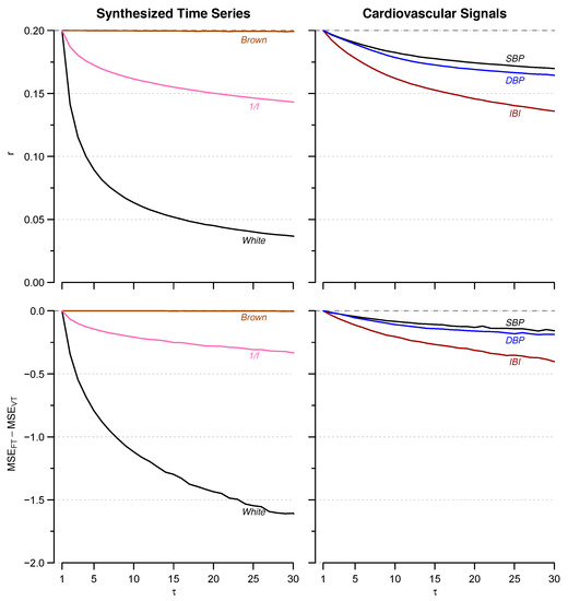
Figure 9.
Relation between changes in the varying tolerance r(τ) (upper panels) and in the difference between fixed- and varying-tolerance estimates of multiscale entropy, MSEFT − MSEVT (lower panels), with increasing τ, for synthesized signals (left) and for real cardiovascular signals (right). The fixed tolerance r = 0.20 used in MSEFT (dashed line in upper panels) is shown as reference.
Based on this analysis, we may predict that the greater MSEVT − MSEFT difference observed for heart rate than for blood pressure (Figure 3) should be associated with a varying tolerance r(τ) decreasing with τ more steeply for IBI than for SBP or DBP. As predicted, this is the trend characterizing our physiological data (Figure 9, right panels).
The vagal modulation of heart rate might explain the different behavior of SD(τ) of IBI compared with SD(τ) of SBP or DBP. In contrast with the sympathetic outflow, the vagal outflow contributes importantly to the heart rate variability and has little or no effects on SBP or DBP dynamics. Selective autonomic blockade showed that the vagal outflow contributes to heart rate variability with a “short-memory” fractal noise while the contribution of the sympathetic outflow is more similar to a long-memory Brownian motion [18]. Therefore, it is conceivable that the steeper decrease of SD(τ) and the greater discrepancy between MSEVT and MSEFT estimates for IBI compared to SBP and DBP, derive from vagal modulations of heart rate with “short-memory” fractal dynamics. This would also explain why previous studies that compared MSEVT and MSEFT in congestive heart failure patients [6] or in a rat model of hypertension and heart failure [7] did not find differences as significant as in our study. In fact, this type of patient and this animal model are both characterized by low vagal tone, compared to our healthy volunteers.
Our analysis allows extending similar conclusions to other types of physiological time series and we may expect substantial differences between MSEVT and MSEFT estimates whenever “short-memory” fractal processes prevail on “long-memory” fractal components. However, this aspect of signal dynamics could not be predicted easily because, besides the cardiovascular time series, other physiological signals, like the electroencephalogram, also may be characterized by fractal components that depend on the observational scales [19], and these signals may change between fractional Gaussian noises and fractional Brownian motions under specific physiological or clinical conditions. Therefore, future studies are needed to evaluate whether differences between the two approaches may be relevant for other physiological time series or under specific physiological or clinical conditions.
Since the choice between MSEVT and MSEFT may have an important influence on the analysis of cardiovascular signals, the question that arises is what estimator should we use? If one considers a white noise process {x(j)}, the coarse-grained series of order τ defined by Equation (2) is again a white noise process, and therefore its entropy should be exactly the same of the original series at any coarse-graining level. The varying tolerance approach estimates a constant entropy level among all scales for white noise, and therefore MSEVT should be preferred to MSEFT if one wants to estimate the correct level of entropy of a coarse-grained series. However, in physiological or clinical studies the interest is to decompose the unpredictability of the cardiovascular series separately by temporal scales. If one assumes that a process “without memory”, such as the white noise, concentrates the unpredictability at the shortest scales, while a long memory process, like the “1/f” noise, distributes unpredictability over a large range of scales, then MSEFT appears to be more useful than MSEVT for describing this aspect of cardiovascular complexity. In fact, MSEVT entrains the irregularity of white noise from the shortest to the largest scales by adjusting the tolerance as SD(τ) decreases, but in this way the multiscale profile of white noise results to be very similar to the profile of “1/f” noise (Figure 1, right). Therefore, multiscale analysis provides little information only for distinguishing the two processes in addition to the difference in Sampen, at scale 1. This is not the case for MSEFT: white noise and “1/f” noise not only have different entropy at scale 1, but also a different entropy distribution among scales.
Moreover, because of the entraining of irregularity from short to long scales, the interpretation of physiological differences may be more problematic if MSEVT rather than MSEFT is used. In fact, let’s consider the sex differences in multiscale entropy of IBI and SBP (Figure 6 and Figure 7). If MSEFT is used, sex differences affect a narrow range of IBI scales around τ = 5 beats, and all the SBP scales. This would suggest that they regard a short-memory process for IBI and a long-memory process for SBP. By contrast, if MSEVT is used, significant sex differences extend to all IBI scales greater than 3. This makes difficult to distinguish whether they are due to the entraining of entropy from the shorter to the larger scales, or to sex differences in a long-memory process, as it seems to be the case for SBP.
A further aspect that would make MSEFT preferable to MSEVT is that the dispersion of the estimates for synthesized (Figure 2) and real (Figure 4) signals is lower for the fixed-tolerance estimator. This suggests that MSEFT may give more precise estimates of multiscale entropy.
In conclusion, although our work provided evidence suggesting that MSEFT could be preferable to MSEVT, it is likely that the choice between fixed- and varying-tolerance will remain a matter of debate. Since our data showed that the choice between the two estimators may influence results and interpretation of the analysis of cardiovascular signals, particularly for heart rate, we recommend that future studies on heart rate variability explicitly indicate whether a fixed- or a varying-tolerance approach is considered, possibly reporting whether the two approaches provide discrepant results.
Acknowledgments
The research was funded by the participating Institutions, without any external support. Open access publication was supported by funds of the “Ricerca Corrente 2015–2017” grant from Italian Ministry of Health.
Author Contributions
Paolo Castiglioni and Andrea Faini designed the work, analyzed and interpreted the data, created the software used in the work and drafted the manuscript. Paolo Coruzzi and Matteo Bini acquired the data and interpreted the results. Gianfranco Parati contributed to data interpretation and manuscript revision. All authors have read and approved the final manuscript.
Conflicts of Interest
The authors declare no conflict of interest.
Appendix A. Variability of MSE Estimates at Large τ
When the time series is coarse grained for evaluating MSE at scales τ > 1, the number of samples available for SampEn estimation decreases from N to int (N/τ), possibly decreasing the quality of the estimate in terms of accuracy (bias of the estimate) and precision (variability of the estimate). While we may exclude bias at higher scales because theoretically, MSEVT of white noise should be constant at all τ and we found a constant MSEVT without any sign of bias (Figure 1b); the variability of the estimates increases with τ, as reported in Figure 2. Although the minimal number of samples for a reliable SampEn estimation is still an open question, the group of Costa et al. who originally proposed MSE extended the estimation for embedding dimension m = 2 up to scales τ that allow evaluating SampEn on at least 1000 points [5], therefore implicitly suggesting that similar lengths of the coarse-grained series should be considered for reliable estimates. In our work, the length of the coarse-grained series at the higher τ is 28% only the length suggested in [5], but we think that our estimates may provide similarly reliable results.
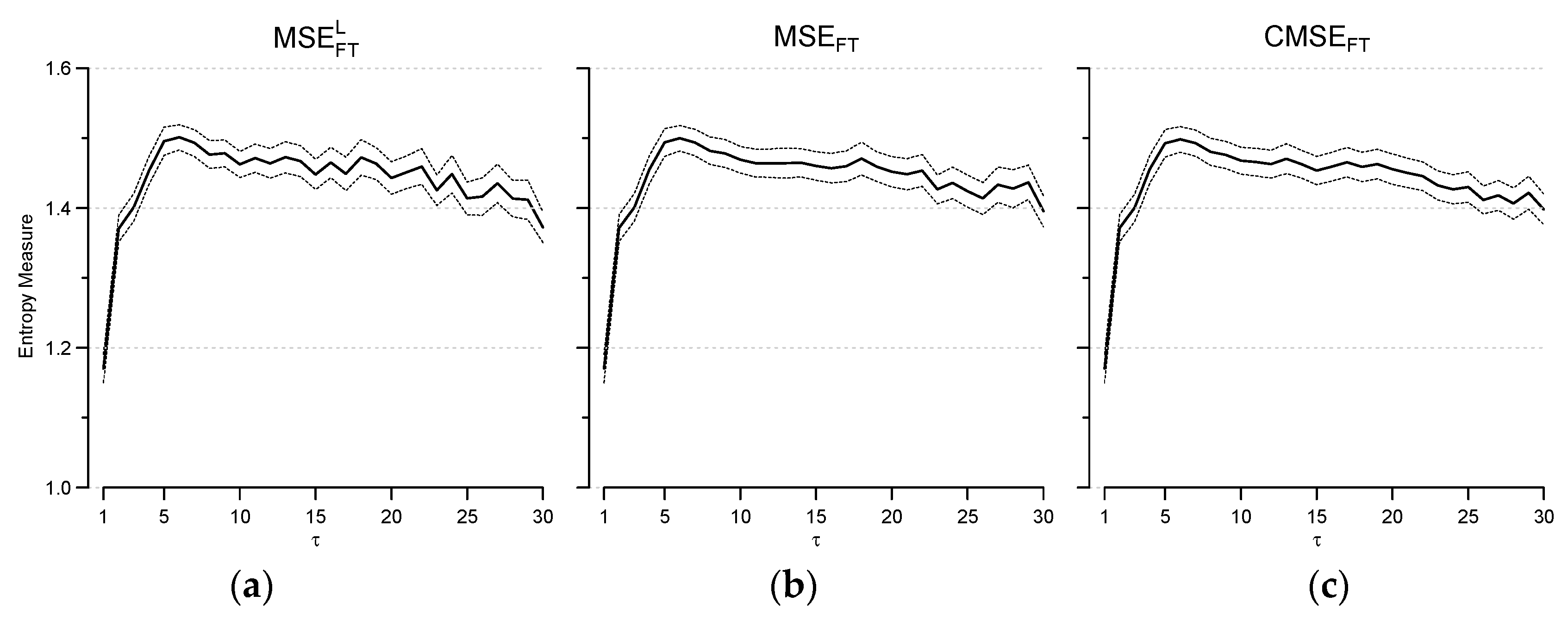
In fact, our MSEFT and MSEVT estimators average MSEs calculated after both left-sided and right-sided coarse graining (Equations (4) and (5)), and this allows better extracting the information from the original series. Our approach is somehow similar to the Composite MSE estimator proposed by Wu et al. [8]. In fact, the Composite MSE at each scale τ is the average of MSEs calculated from the coarse-grained series derived by shifting repeatedly the starting point of coarse graining by one sample. As in our approach, this allows retrieving the information contained in the last segment of data discarded when coarse graining starts from the first sample. Figure A1 compares the average over the whole group of participants of MSEFT of IBI as obtained with our approach (central panel), with the left-sided MSE corresponding to the traditional coarse graining (left panel) and with Composite MSE (right panel). Clearly, both our MSEFT approach and the Composite MSE approach reduce appreciably the instability of the estimate at the larger τ. Actually, it has been shown that the SD of Composite MSE is about 60% the SD of the traditional MSE estimator when the length of the coarse grained series is similar to the length we have for τ = 30 (Table 1 of [8]). However, we decided to implement the average between left-sided and right-sided MSE rather than the Composite MSE because of its better computational efficiency. Simulations with the synthesized series of Figure 1 showed that MSE calculation up to τ = 30 and m from 1 to 3 requires 4% only more time by MSEFT and 24% more time by Composite MSE, in comparison to the traditional estimation based on the left-sided coarse graining only.
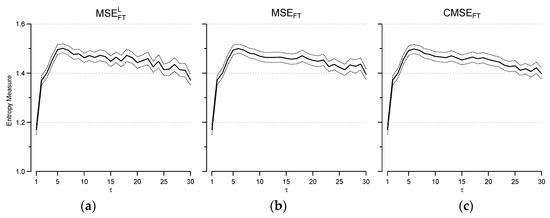
Figure A1.
Mean ± 95% confidence intervals of the mean over the group (N = 84) for fixed-tolerance MSE of IBI and m = 3 estimated by left-sided coarse grainings only (MSELFT, panel (a)); by averaging left- and right-sided coarse grainings (MSEFT, panel (b)); and by Composite MSE (CMSEFT, panel (c)).
In addition, we also found that the quality of the estimate is better for lower embedding dimensions, and for this reason the comparison among signals and between sexes was performed for m = 1, which appears to provide more stable estimates than for m = 2, this latter being the embedding dimension used in [5]. Therefore, even at the largest scales the quality of our MSE estimates may be considered comparable to that proposed in previous works.
References
- Richman, J.S.; Moorman, J.R. Physiological time-series analysis using approximate entropy and sample entropy. Am. J. Physiol. Heart Circ. Physiol. 2000, 278, H2039–H2049. [Google Scholar] [PubMed]
- Pincus, S.M.; Huang, W.M. Approximate entropy: Statistical properties and applications. Commun. Stat. Theory Methods 1992, 21, 3061–3077. [Google Scholar] [CrossRef]
- Costa, M.; Goldberger, A.L.; Peng, C.K. Multiscale entropy analysis of complex physiologic time series. Phys. Rev. Lett. 2002, 89, 068102. [Google Scholar] [CrossRef] [PubMed]
- Nikulin, V.V.; Brismar, T. Comment on “Multiscale entropy analysis of complex physiologic time series”. Phys. Rev. Lett. 2004, 92, 089803. [Google Scholar] [CrossRef] [PubMed]
- Costa, M.; Goldberger, A.L.; Peng, C.K. Multiscale entropy analysis of biological signals. Phys. Rev. E 2005, 71, 021906. [Google Scholar] [CrossRef] [PubMed]
- Angelini, L.; Maestri, R.; Marinazzo, D.; Nitti, L.; Pellicoro, M.; Pinna, G.D.; Stramaglia, S.; Tupputi, S.A. Multiscale analysis of short term heart beat interval, arterial blood pressure, and instantaneous lung volume time series. Artif. Intell. Med. 2007, 41, 237–250. [Google Scholar] [CrossRef] [PubMed]
- Silva, L.E.; Lataro, R.M.; Castania, J.A.; da Silva, C.A.; Valencia, J.F.; Murta, L.O., Jr.; Salgado, H.C.; Fazan, R., Jr.; Porta, A. Multiscale entropy analysis of heart rate variability in heart failure, hypertensive, and sinoaortic-denervated rats: Classical and refined approaches. Am. J. Physiol. Regul. Integr. Comp. Physiol. 2016, 311, R150–R156. [Google Scholar] [CrossRef] [PubMed]
- Wu, S.D.; Wu, C.W.; Lin, S.G.; Wang, C.C.; Lee, K.Y. Time Series Analysis Using Composite Multiscale Entropy. Entropy 2013, 15, 1069–1084. [Google Scholar] [CrossRef]
- Wu, S.D.; Wu, C.W.; Lin, S.G.; Lee, K.Y.; Peng, C.K. Analysis of complex time series using refined composite multiscale entropy. Phys. Lett. A 2014, 378, 1369–1374. [Google Scholar] [CrossRef]
- Chang, Y.C.; Wu, H.T.; Chen, H.R.; Liu, A.B.; Yeh, J.J.; Lo, M.T.; Tsao, J.H.; Tang, C.J.; Tsai, I.T.; Sun, C.K. Application of a Modified Entropy Computational Method in Assessing the Complexity of Pulse Wave Velocity Signals in Healthy and Diabetic Subjects. Entropy 2014, 16, 4032–4043. [Google Scholar] [CrossRef]
- Wu, S.D.; Wu, C.W.; Lee, K.Y.; Lin, S.G. Modified multiscale entropy for short-term time series analysis. Phys. A Stat. Mech. Appl. 2013, 392, 5865–5873. [Google Scholar] [CrossRef]
- Valencia, J.F.; Porta, A.; Vallverdu, M.; Claria, F.; Baranowski, R.; Orlowska-Baranowska, E.; Caminal, P. Refined multiscale entropy: Application to 24-h Holter recordings of heart period variability in healthy and aortic stenosis subjects. IEEE Trans. Biomed. Eng. 2009, 56, 2202–2213. [Google Scholar] [CrossRef] [PubMed]
- Chen, W.; Wang, Z.; Xie, H.; Yu, W. Characterization of surface EMG signal based on fuzzy entropy. IEEE Trans. Neural Syst. Rehabil. Eng. 2007, 15, 266–272. [Google Scholar] [CrossRef] [PubMed]
- Castiglioni, P.; Parati, G.; Lazzeroni, D.; Bini, M.; Faini, A.; Brambilla, L.; Brambilla, V.; Coruzzi, P. Hemodynamic and Autonomic Response to Different Salt Intakes in Normotensive Individuals. J. Am. Heart Assoc. 2016, 5. [Google Scholar] [CrossRef] [PubMed]
- Coruzzi, P.; Parati, G.; Brambilla, L.; Brambilla, V.; Gualerzi, M.; Novarini, A.; Castiglioni, P.; Di Rienzo, M. Effects of salt sensitivity on neural cardiovascular regulation in essential hypertension. Hypertension 2005, 46, 1321–1326. [Google Scholar] [CrossRef] [PubMed]
- Goldberger, A.L.; Amaral, L.A.; Glass, L.; Hausdorff, J.M.; Ivanov, P.C.; Mark, R.G.; Mietus, J.E.; Moody, G.B.; Peng, C.K.; Stanley, H.E. PhysioBank, PhysioToolkit, and PhysioNet: Components of a new research resource for complex physiologic signals. Circulation 2000, 101, E215–E220. [Google Scholar] [CrossRef] [PubMed]
- Flyvbjerg, H.; Petersen, H.G. Error estimates on averages of correlated data. J. Chem. Phys. 1989, 91, 461–466. [Google Scholar] [CrossRef]
- Castiglioni, P.; Parati, G.; Di Rienzo, M.; Carabalona, R.; Cividjian, A.; Quintin, L. Scale exponents of blood pressure and heart rate during autonomic blockade as assessed by detrended fluctuation analysis. J. Physiol. 2011, 589, 355–369. [Google Scholar] [CrossRef] [PubMed]
- Castiglioni, P. Self-similarity in Physiological Time Series: New Perspectives from the Temporal Spectrum of Scale Exponents. In Computational Intelligence Methods for Bioinformatics and Biostatistics; Biganzoli, E., Vellido, A., Ambrogi, F., Tagliaferri, R., Eds.; Revised Selected Papers; Springer: Berlin/Heidelberg, Germany, 2012; pp. 164–175. [Google Scholar]
© 2017 by the authors. Licensee MDPI, Basel, Switzerland. This article is an open access article distributed under the terms and conditions of the Creative Commons Attribution (CC BY) license (http://creativecommons.org/licenses/by/4.0/).


