Robust and Sparse Regression via γ-Divergence

Abstract

In high-dimensional data, many sparse regression methods have been proposed. However, they may not be robust against outliers. Recently, the use of density power weight has been studied for robust parameter estimation, and the corresponding divergences have been discussed. One such divergence is the $\gamma$-divergence, and the robust estimator using the $\gamma$-divergence is known for having a strong robustness. In this paper, we extend the $\gamma$-divergence to the regression problem, consider the robust and sparse regression based on the $\gamma$-divergence and show that it has a strong robustness under heavy contamination even when outliers are heterogeneous. The loss function is constructed by an empirical estimate of the $\gamma$-divergence with sparse regularization, and the parameter estimate is defined as the minimizer of the loss function. To obtain the robust and sparse estimate, we propose an efficient update algorithm, which has a monotone decreasing property of the loss function. Particularly, we discuss a linear regression problem with $L_1$ regularization in detail. In numerical experiments and real data analyses, we see that the proposed method outperforms past robust and sparse methods.

1. Introduction

In high-dimensional data, sparse regression methods have been intensively studied. The Lasso [1] is a typical sparse linear regression method with $L_1$ regularization, but is not robust against outliers. Recently, robust and sparse linear regression methods have been proposed. The robust least angle regression (RLARS) [2] is a robust version of LARS [3], which replaces the sample correlation by a robust estimate of correlation in the update algorithm. The sparse least trimmed squares (sLTS) [4] is a sparse version of the well-known robust linear regression method LTS [5] based on the trimmed loss function with $L_1$ regularization.

Recently, the robust parameter estimation using density power weight has been discussed by Windham [6], Basu et al. [7], Jones et al. [8], Fujisawa and Eguchi [9], Basu et al. [10], Kanamori and Fujisawa [11], and so on. The density power weight gives a small weight to the terms related to outliers, and then, the parameter estimation becomes robust against outliers. By virtue of this validity, some applications using density power weights have been proposed in signal processing and machine learning [12,13]. Among them, the $\gamma$-divergence proposed by Fujisawa and Eguchi [9] is known for having a strong robustness, which implies that the latent bias can be sufficiently small even under heavy contamination. The other robust methods including density power-divergence cannot achieve the above property, and the estimator can be affected by the outlier ratio. In addition, to obtain the robust estimate, an efficient update algorithm was proposed with a monotone decreasing property of the loss function.

In this paper, we propose the robust and sparse regression problem based on the $\gamma$-divergence. First, we extend the $\gamma$-divergence to the regression problem. Next, we consider a loss function based on the $\gamma$-divergence with sparse regularization and propose an update algorithm to obtain the robust and sparse estimate. Fujisawa and Eguchi [9] used a Pythagorean relation on the $\gamma$-divergence, but it is not compatible with sparse regularization. Instead of this relation, we use the majorization-minimization algorithm [14]. This idea is deeply considered in a linear regression problem with $L_1$ regularization. The MM algorithm was also adopted in Hirose and Fujisawa [15] for robust and sparse Gaussian graphical modeling. A tuning parameter selection is proposed using a robust cross-validation. We also show a strong robustness under heavy contamination even when outliers are heterogeneous. Finally, in numerical experiments and real data analyses, we show that our method is computationally efficient and outperforms other robust and sparse methods. The R language software package “gamreg”, which we use to implement our proposed method, can be downloaded at http://cran.r-project.org/web/packages/gamreg/.

2. Regression Based on $\mathit{\gamma }$-Divergence

The $\gamma$-divergence was defined for two probability density functions, and its properties were investigated by Fujisawa and Eguchi [9]. In this section, the $\gamma$-divergence is extended to the regression problem, in other words, defined for two conditional probability density functions.

2.1. $\gamma$-Divergence for Regression

We suppose that $g(x,y)$, $g(y|x)$ and $g(x)$ are the underlying probability density functions of $(x,y)$, y given x and x, respectively. Let $f(y|x)$ be another parametric conditional probability density function of y given x. Let us define the $\gamma$-cross-entropy for regression by:

$$\begin{array}{c}{d}_{\gamma }(g(y|x),f(y|x);g(x))\hfill \\ =-\frac{1}{\gamma }log\int \left(\int g(y|x)f{(y|x)}^{\gamma }dy\right)g(x)dx+\frac{1}{1+\gamma }log\int \left(\int f{(y|x)}^{1+\gamma }dy\right)g(x)dx\hfill \\ =-\frac{1}{\gamma }log\int \int f{(y|x)}^{\gamma }g(x,y)dxdy+\frac{1}{1+\gamma }log\int \left(\int f{(y|x)}^{1+\gamma }dy\right)g(x)dxfor\gamma >0.\hfill \end{array}$$

(1)

The $\gamma$-divergence for regression is defined by:

$$\begin{array}{c}{D}_{\gamma }(g(y|x),f(y|x);g(x))=-d_{\gamma }(g(y|x),g(y|x);g(x))+d_{\gamma }(g(y|x),f(y|x);g(x)).\end{array}$$

(2)

The $\gamma$-divergence for regression was first proposed by Fujisawa and Eguchi [9], and many properties were already shown. However, we adopt the definition (2), which is slightly different from the past one, because (2) satisfies the Pythagorean relation approximately (see Section 4).

Theorem 1.

We can show that:

$$\begin{array}{cc}\hfill (\mathrm{i})& D_{\gamma }(g(y|x),f(y|x);g(x))\ge 0,\hfill \\ \hfill (\mathrm{ii})& D_{\gamma }(g(y|x),f(y|x);g(x))=0\iff g(y|x)=f(y|x)(\mathrm{a}.\mathrm{e}.),\hfill \\ \hfill (\mathrm{iii})& \underset{\gamma \to 0}{lim}{D}_{\gamma }(g(y|x),f(y|x);g(x))=\int D_{KL}(g(y|x),f(y|x))g(x)dx,\hfill \end{array}$$

where $D_{KL}(g(y|x),f(y|x))=\int g(y|x)logg(y|x)dy-\int g(y|x)logf(y|x)dy.$

The proof is in Appendix A. In what follows, we refer to the regression based on the $\gamma$-divergence as the $\gamma$-regression.

2.2. Estimation for $\gamma$-Regression

Let $f(y|x;\theta )$ be the conditional probability density function of y given x with parameter $\theta$. The target parameter can be considered by:

$$\begin{array}{cc}\hfill {\theta }_{\gamma }^{*}& =\underset{\theta }{\mathrm{argmin}}{D}_{\gamma }(g(y|x),f(y|x;\theta );g(x))\hfill \\ & =\underset{\theta }{\mathrm{argmin}}{d}_{\gamma }(g(y|x),f(y|x;\theta );g(x)).\hfill \end{array}$$

(3)

When $g(y|x)=f(y|x;{\theta }^{*})$, we have ${\theta }_{\gamma }^{*}={\theta }^{*}$.

Let $(x_1,y_1),\dots ,(x_n,y_n)$ be the observations randomly drawn from the underlying distribution $g(x,y)$. Using the formula (1), the $\gamma$-cross-entropy for regression, $d_{\gamma }(g(y|x),f(y|x;\theta );g(x))$, can be empirically estimated by:

$$\begin{array}{c}{\overline{d}}_{\gamma }(f(y|x;\theta ))=-\frac{1}{\gamma }log\left\{\frac{1}{n}\sum _{i=1}^{n}f{(y_i|x_i;\theta )}^{\gamma }\right\}+\frac{1}{1+\gamma }log\left\{\frac{1}{n}\sum _{i=1}^n\int f{(y|x_i;\theta )}^{1+\gamma }dy\right\}.\hfill \end{array}$$

By virtue of (3), we define the $\gamma$-estimator by:

$$\begin{array}{c}\hfill {\widehat{\theta }}_{\gamma }=\underset{\theta }{\mathrm{argmin}}{\overline{d}}_{\gamma }(f(y|x;\theta )).\end{array}$$

(4)

In a similar way as in Fujisawa and Eguchi [9], we can show the consistency of ${\widehat{\theta }}_{\gamma }$ to ${\theta }_{\gamma }^{*}$ under some conditions.

Here, we briefly show why the $\gamma$-estimator is robust. Suppose that $y_1$ is an outlier. The conditional probability density $f(y_1|x_1;\theta )$ can be expected to be sufficiently small. We see from $f(y_1|x_1;\theta )\approx 0$ and (4) that:

$$\begin{array}{c}\underset{\theta }{\mathrm{argmin}}{\overline{d}}_{\gamma }(f(y|x;\theta ))\hfill \\ =\underset{\theta }{\mathrm{argmin}}-\frac{1}{\gamma }log\left\{\frac{1}{n}\sum _{i=1}^{n}f{(y_i|x_i;\theta )}^{\gamma }\right\}+\frac{1}{1+\gamma }log\left\{\frac{1}{n}\sum _{i=1}^n\int f{(y|x_i;\theta )}^{1+\gamma }dy\right\}\hfill \\ \approx \underset{\theta }{\mathrm{argmin}}-\frac{1}{\gamma }log\left\{\frac{1}{n-1}\sum _{i=2}^{n}f{(y_i|x_i;\theta )}^{\gamma }\right\}+\frac{1}{1+\gamma }log\left\{\frac{1}{n}\sum _{i=1}^n\int f{(y|x_i;\theta )}^{1+\gamma }dy\right\}.\hfill \end{array}$$

Therefore, the term $f(y_1|x_1;\theta )$ is naturally ignored in (4). However, for the KL-divergence, $logf(y_1|x_1;\theta )$ diverges from $f(y_1|x_1;\theta )\approx 0$. That is why the KL-divergence is not robust. The theoretical robust properties are presented in Section 4.

Moreover, the empirical estimation of the $\gamma$-cross-entropy with a penalty term can be given by:

$$\begin{array}{c}\hfill L_{\gamma }(\theta ;\lambda )={\overline{d}}_{\gamma }(f(y|x;\theta ))+\lambda P(\theta ),\end{array}$$

where $P(\theta )$ is a penalty for parameter $\theta$ and $\lambda$ is a tuning parameter for the penalty term. As an example of the penalty term, we can consider $L_1$ (Lasso, Tibshirani [1]), elasticnet [16], group Lasso [17], fused Lasso [18], and so on. The sparse $\gamma$-estimator can be proposed by:

$$\begin{array}{c}\hfill {\widehat{\theta }}_S=\underset{\theta }{\mathrm{argmin}}{L}_{\gamma }(\theta ;\lambda ).\end{array}$$

To obtain the minimizer, we propose the iterative algorithm by the majorization-minimization algorithm (MM algorithm) [14].

3. Parameter Estimation Procedure

3.1. MM Algorithm for Sparse $\gamma$-Regression

The MM algorithm is constructed as follows. Let $h(\eta )$ be the objective function. Let us prepare the majorization function $h_{MM}$ satisfying:

$$\begin{array}{cc}\hfill h_{MM}({\eta }^{(m)}|{\eta }^{(m)})& =h({\eta }^{(m)}),\hfill \\ \hfill h_{MM}(\eta |{\eta }^{(m)})& \ge h(\eta )\mathrm{for} \mathrm{all} \eta ,\hfill \end{array}$$

where ${\eta }^{(m)}$ is the parameter of the m-th iterative step for $m=0,1,2,\dots$ Let us consider the iterative algorithm by:

$$\begin{array}{c}\hfill {\eta }^{(m+1)}=\underset{\eta }{\mathrm{argmin}}{h}_{MM}(\eta |{\eta }^{(m)}).\end{array}$$

Then, we can show that the objective function $h(\eta )$ monotonically decreases at each step, because:

$$\begin{array}{cc}\hfill h({\eta }^{(m)})& =h_{MM}({\eta }^{(m)}|{\eta }^{(m)})\hfill \\ & \ge h_{MM}({\eta }^{(m+1)}|{\eta }^{(m)})\hfill \\ & \ge h({\eta }^{(m+1)}).\hfill \end{array}$$

Note that ${\eta }^{(m+1)}$ does not necessarily have to be the minimizer of $h_{MM}(\eta |{\eta }^{(m)})$. We only need:

$$\begin{array}{c}\hfill h_{MM}({\eta }^{(m)}|{\eta }^{(m)})\ge h_{MM}({\eta }^{(m+1)}|{\eta }^{(m)}).\end{array}$$

We construct the majorization function for the sparse $\gamma$-regression by the following inequality:

$$\begin{array}{cc}\hfill \kappa (z^T\eta )& \le \sum _i\frac{z_i{\eta }_i^{(m)}}{z^T{\eta }^{(m)}}\kappa \left[{\eta }_i\frac{z^T{\eta }^{(m)}}{{\eta }_i^{(m)}}\right],\hfill \end{array}$$

(5)

where $\kappa (u)$ is a convex function, $z={(z_1,\dots ,z_n)}^T$, $\eta ={({\eta }_1,\dots ,{\eta }_n)}^T$, ${\eta }^{(m)}={({\eta }_1^{(m)},\dots ,{\eta }_n^{(m)})}^T$, and $z_i$, ${\eta }_i$ and ${\eta }_i^{(m)}$ are positive. The inequality (5) holds from Jensen’s inequality. Here, we take $z_i=\frac{1}{n}$, ${\eta }_i=f{(y_i|x_i;\theta )}^{\gamma }$, ${\eta }_i^{(m)}=f{(y_i|x_i;{\theta }^{(m)})}^{\gamma }$, and $\kappa (u)=-logu$ in (5). We can propose the majorization function as follows:

$$\begin{array}{c}h(\theta )\hfill \\ =L_{\gamma }(\theta ;\lambda )\hfill \\ =-\frac{1}{\gamma }log\left\{\frac{1}{n}\sum _{i=1}^{n}f{(y_i|x_i;\theta )}^{\gamma }\right\}+\frac{1}{1+\gamma }log\left\{\frac{1}{n}\sum _{i=1}^n\int f{(y|x_i;\theta )}^{1+\gamma }dy\right\}+\lambda P(\theta )\hfill \\ \le -\frac{1}{\gamma }\sum _{i=1}^n{\alpha }_i^{(m)}log\left\{f{(y_i|x_i;\theta )}^{\gamma }\frac{\frac{1}{n}{\sum }_{l=1}^{n}f{(y_l|x_l;{\theta }^{(m)})}^{\gamma }}{f{(y_i|x_i;{\theta }^{(m)})}^{\gamma }}\right\}\hfill \\ +\frac{1}{1+\gamma }log\left\{\frac{1}{n}\sum _{i=1}^n\int f{(y|x_i;\theta )}^{1+\gamma }dy\right\}+\lambda P(\theta )\hfill \\ =-\sum _{i=1}^n{\alpha }_i^{(m)}logf(y_i|x_i;\theta )+\frac{1}{1+\gamma }log\left\{\frac{1}{n}\sum _{i=1}^n\int f{(y|x_i;\theta )}^{1+\gamma }dy\right\}+\lambda P(\theta )\hfill \\ +const\hfill \\ =h_{MM}(\theta |{\theta }^{(m)})+const,\hfill \end{array}$$

where ${\alpha }_i^{(m)}=\frac{f{(y_i|x_i;{\theta }^{(m)})}^{\gamma }}{{\sum }_{l=1}^{n}f{(y_l|x_l;{\theta }^{(m)})}^{\gamma }}$ and $const$ is a term that does not depend on the parameter $\theta$.

The first term on the original target function $h(\theta )$ is a mixture type of densities, which is not easy to optimize, while the first term on $h_{MM}(\theta |{\theta }^{(m)})$ is a weighted log-likelihood, which is often easy to optimize.

3.2. Sparse $\gamma$-Linear Regression

Let $f(y|x;\theta )$ be the conditional density with $\theta =({\beta }_0,\beta ,{\sigma }^2)$, given by:

$$\begin{array}{c}\hfill f(y|x;\theta )=\varphi (y;{\beta }_0+x^T\beta ,{\sigma }^2),\end{array}$$

where $\varphi (y;\mu ,{\sigma }^2)$ is the normal density with mean parameter $\mu$ and variance parameter ${\sigma }^2$. Suppose that $P(\theta )$ is the $L_1$ regularization ${||\beta ||}_1$. After a simple calculation, we have:

$$\begin{array}{c}\hfill h_{MM}(\theta |{\theta }^{(m)})=\frac{1}{2(1+\gamma )}log{\sigma }^2+\frac{1}{2}\sum _{i=1}^n{\alpha }_i^{(m)}\frac{{(y_i-{\beta }_0-x_i^T\beta )}^2}{{\sigma }^2}+{\lambda ||\beta ||}_1.\end{array}$$

(6)

This function is easy to optimize by an update algorithm. For a fixed value of ${\sigma }^2$, the function $h_{MM}$ is almost the same as Lasso except for the weight, so that it can be updated using the coordinate decent algorithm with a decreasing property of the loss function. For a fixed value of ${({\beta }_0,{\beta }^T)}^T$, the function $h_{MM}$ is easy to minimize. Consequently, we can obtain the update algorithm in Algorithm 1 with the decreasing property:

$$\begin{array}{c}\hfill h_{MM}({\theta }^{(m+1)}|{\theta }^{(m)})\le h_{MM}({\theta }^{(m)}|{\theta }^{(m)}).\end{array}$$

Algorithm 1 Sparse $\gamma$-linear regression.

Require: ${\beta }_0^{(0)},{\beta }^{(0)},{{\sigma }^2}^{(0)}$  repeat $m=0,1,2,\dots$   ${\alpha }_i^{(m)}\leftarrow \frac{\varphi {(y_i;{{\beta }_0}^{(m)}+x_i^T{\beta }^{(m)},{{\sigma }^2}^{(m)})}^{\gamma }}{{\sum }_{l=1}^n\varphi {(y_l;{{\beta }_0}^{(m)}+{x_l}^T{\beta }^{(m)},{{\sigma }^2}^{(m)})}^{\gamma }}(i=1,2,\dots ,n).$   ${{\beta }_0}^{(m+1)}\leftarrow {\sum }_{i=1}^n{\alpha }_i^{(m)}(y_i-{x_i}^T{\beta }^{(m)}).$   for $\mathbf{do}j=1,\dots ,p$    ${{\beta }_j}^{(m+1)}\leftarrow \frac{S\left({\sum }_{i=1}^n{\alpha }_i^{(m)}(y_i-{\beta }_0^{(m+1)}-r_{i,-j}^{(m)})x_{ij},{{\sigma }^2}^{(m)}\lambda \right)}{\left({\sum }_{i=1}^n{\alpha }_i^{(m)}{x}_{ij}^2\right)},$    where $S(t,\lambda )=\mathrm{sign}(t){(|t|-\lambda )}_{+}$ and $r_{i,-j}^{(m)}={\sum }_{k\ne j}{x}_{ik}({\mathbb{1}}_{(k<j)}{\beta }_k^{(m+1)}+{\mathbb{1}}_{(k>j)}{\beta }_k^{(m)})$.   ${{\sigma }^2}^{(m+1)}\leftarrow (1+\gamma ){\sum }_{i=1}^n{\alpha }_i^{(m)}{(y_i\alpha -{\beta }_0^{(m+1)}\alpha -x_i^T{\beta }^{(m+1)})}^2.$  until convergence Ensure: ${\widehat{\beta }}_0,\widehat{\beta },{\widehat{\sigma }}^2$

It should be noted that $h_{MM}$ is convex with respect to parameter ${\beta }_0$, $\beta$ and has the global minimum with respect to parameter ${\sigma }^2$, but the original objective function h is not convex with respect to them, so that the initial points of Algorithm 1 are important. This issue is discussed in Section 5.4.

In practice, we also use the active set strategy [19] in the coordinate decent algorithm for updating ${\beta }^{(m)}$. The active set consists of the non-zero coordinates of ${\beta }^{(m)}$. Specifically, for a given ${\beta }^{(m)}$, we only update the non-zero coordinates of ${\beta }^{(m)}$, until they are converged. Then, the non-active set parameter estimates are updated once. When they remain zero, the coordinate descent algorithm stops. If some of them do not remain zero, those are added to the active set, and the coordinate descent algorithm continues.

3.3. Robust Cross-Validation

In sparse regression, a regularization parameter is often selected via a criterion. Cross-validation is often used for selecting the regularization parameter. Ordinal cross-validation is based on the squared error, and it can also be constructed using the KL-cross-entropy with the normal density. However, the ordinal cross-validation will fail due to outliers. Therefore, we propose the robust cross-validation based on the $\gamma$-cross-entropy. Let ${\widehat{\theta }}_{\gamma }$ be the robust estimate based on the $\gamma$-cross-entropy. The cross-validation based on the $\gamma$-cross-entropy can be given by:

$$\begin{array}{c}\mathrm{RoCV}(\lambda )\hfill \\ =-\frac{1}{{\gamma }_0}log\left\{\frac{1}{n}\sum _{i=1}^{n}f{(y_i|x_i;{\widehat{\theta }}_{\gamma }^{[-i]})}^{{\gamma }_0}\right\}+\frac{1}{1+{\gamma }_0}log\left\{\frac{1}{n}\sum _{i=1}^n\int f{(y|x_i;{\widehat{\theta }}_{\gamma }^{[-i]})}^{1+{\gamma }_0}dy\right\},\hfill \end{array}$$

where ${\widehat{\theta }}_{\gamma }^{[-i]}$ is the $\gamma$-estimator deleting the i-th observation and ${\gamma }_0$ is an appropriate tuning parameter. We can also adopt the K-fold cross-validation to reduce the computational task [20].

Here, we give a small modification of the above. We often focus only on the mean structure for prediction, not on the variance parameter. Therefore, in this paper, ${\widehat{\theta }}_{\gamma }^{[-i]}=\left({\widehat{\beta }}_{\gamma }^{[-i]},{\widehat{{\sigma }^2}}_{\gamma }^{[-i]}\right)$ is replaced by $\left({\widehat{\beta }}_{\gamma }^{[-i]},{\widehat{{\sigma }^2}}_{fix}\right)$. In numerical experiments and real data analyses, we used ${{\sigma }^2}^{(0)}$ as ${\sigma }_{fix}^2$.

4. Robust Properties

In this section, the robust properties are presented from two viewpoints of latent bias and Pythagorean relation. The latent bias was discussed in Fujisawa and Eguchi [9] and Kanamori and Fujisawa [11], which is described later. Using the results obtained there, the Pythagorean relation is shown in Theorems 2 and 3.

Let $f^{*}(y|x)=f_{{\theta }^{*}}(y|x)=f(y|x;{\theta }^{*})$ and $\delta (y|x)$ be the target conditional probability density function and the contamination conditional probability density function related to outliers, respectively. Let $ϵ$ and $ϵ(x)$ denote the outlier ratios, which are independent of and dependent on x, respectively. Under homogeneous and heterogeneous contaminations, we suppose that the underlying conditional probability density function can be expressed as:

$$\begin{array}{cc}\hfill g(y|x)& =(1-ϵ)f(y|x;{\theta }^{*})+ϵ\delta (y|x),\hfill \\ \hfill g(y|x)& =(1-ϵ(x))f(y|x;{\theta }^{*})+ϵ(x)\delta (y|x).\hfill \end{array}$$

Let:

$$\begin{array}{c}\hfill {\nu }_{f,\gamma }(x)={\left\{\int \delta (y|x)f{(y|x)}^{\gamma }dy\right\}}^{\frac{1}{\gamma }}(\gamma >0),\end{array}$$

and let:

$$\begin{array}{c}\hfill {\nu }_{f,\gamma }={\left\{\int {\nu }_{f,\gamma }{(x)}^{\gamma }g(x)dx\right\}}^{\frac{1}{\gamma }}.\end{array}$$

Here, we assume that:

$$\begin{array}{c}\hfill {\nu }_{f_{{\theta }^{*}},\gamma }\approx 0,\end{array}$$

which implies that ${\nu }_{f_{{\theta }^{*}},\gamma }(x)\approx 0$ for any x (a.e.) and illustrates that the contamination conditional probability density function $\delta (y|x)$ lies on the tail of the target conditional probability density function $f(y|x;{\theta }^{*})$. For example, if $\delta (y|x)$ is the Dirac function at the outlier $y_{†}(x)$ given x, then we have ${\nu }_{f_{{\theta }^{*}},\gamma }(x)=f(y_{†}(x)|x;{\theta }^{*})$, which should be sufficiently small because $y_{†}(x)$ is an outlier. In this section, we show that ${\theta }_{\gamma }^{*}-{\theta }^{*}$ is expected to be small even if $ϵ$ or $ϵ(x)$ is not small. To make the discussion easier, we prepare the monotone transformation of the $\gamma$-cross-entropy for regression by:

$$\begin{array}{c}{\tilde{d}}_{\gamma }(g(y|x),f(y|x;\theta );g(x))\hfill \\ =-exp\left\{-\gamma d_{\gamma }(g(y|x),f(y|x;\theta );g(x))\right\}\hfill \\ =-\frac{\int \left(\int g(y|x)f{(y|x;\theta )}^{\gamma }dy\right)g(x)dx}{{\left\{\int \left(\int f{(y|x;\theta )}^{1+\gamma }dy\right)g(x)dx\right\}}^{\frac{\gamma }{1+\gamma }}}.\hfill \end{array}$$

4.1. Homogeneous Contamination

Here, we provide the following proposition, which was given in Kanamori and Fujisawa [11].

Proposition 1.

$$\begin{array}{c}{\tilde{d}}_{\gamma }(g(y|x),f(y|x;\theta );g(x))\hfill \\ =(1-ϵ){\tilde{d}}_{\gamma }(f(y|x;{\theta }^{*}),f(y|x;\theta );g(x))-\frac{ϵ{\nu }_{f_{\theta },\gamma }^{\gamma }}{{\left\{\int \left(\int f{(y|x;\theta )}^{1+\gamma }dy\right)g(x)dx\right\}}^{\frac{\gamma }{1+\gamma }}}.\hfill \end{array}$$

Recall that ${\theta }_{\gamma }^{*}$ and ${\theta }^{*}$ are also the minimizers of ${\tilde{d}}_{\gamma }(g(y|x),f(y|x;\theta );g(x))$ and ${\tilde{d}}_{\gamma }(f(y|x;{\theta }^{*})$, $f(y|x;\theta );g(x))$, respectively. We can expect ${\nu }_{f_{\theta },\gamma }\approx 0$ from the assumption ${\nu }_{f_{{\theta }^{*}},\gamma }\approx 0$ if the tail behavior of $f(y|x;\theta )$ is close to that of $f(y|x;{\theta }^{*})$. We see from Proposition 1 and the condition ${\nu }_{f_{\theta },\gamma }\approx 0$ that:

$$\begin{array}{cc}\hfill {\theta }_{\gamma }^{*}& =\underset{\theta }{\mathrm{argmin}}{\tilde{d}}_{\gamma }(g(y|x),f(y|x;\theta );g(x))\hfill \\ & =\underset{\theta }{\mathrm{argmin}}\left[(1-ϵ){\tilde{d}}_{\gamma }(f(y|x;{\theta }^{*}),f(y|x;\theta );g(x))\right.\hfill \\ & \left.-\frac{ϵ{\nu }_{f_{\theta },\gamma }^{\gamma }}{{\left\{\int \left(\int f{(y|x;\theta )}^{1+\gamma }dy\right)g(x)dx\right\}}^{\frac{\gamma }{1+\gamma }}}\right]\hfill \\ & \approx \underset{\theta }{\mathrm{argmin}}(1-ϵ){\tilde{d}}_{\gamma }(f(y|x;{\theta }^{*}),f(y|x;\theta );g(x))\hfill \\ & ={\theta }^{*}.\hfill \end{array}$$

Therefore, under homogeneous contamination, it can be expected that the latent bias ${\theta }_{\gamma }^{*}-{\theta }^{*}$ is small even if $ϵ$ is not small. Moreover, we can show the following theorem, using Proposition 1.

Theorem 2.

Let $\nu =max\{{\nu }_{f_{\theta },\gamma },{\nu }_{f_{{\theta }^{*}},\gamma }\}$. Then, the Pythagorean relation among $g(y|x)$, $f(y|x;{\theta }^{*})$, $f(y|x;\theta )$ approximately holds:

$$\begin{array}{c}{D}_{\gamma }(g(y|x),f(y|x;\theta );g(x))-D_{\gamma }(g(y|x),f(y|x;{\theta }^{*});g(x))\hfill \\ =D_{\gamma }(f(y|x;{\theta }^{*}),f(y|x;\theta );g(x))+O({\nu }^{\gamma }).\hfill \end{array}$$

The proof is in Appendix A. The Pythagorean relation implies that the minimization of the divergence from $f(y|x;\theta )$ to the underlying conditional probability density function $g(y|x)$ is approximately the same as that to the target conditional probability density function $f(y|x;{\theta }^{*})$. Therefore, under homogeneous contamination, we can see why our proposed method works well in terms of the minimization of the $\gamma$-divergence.

4.2. Heterogeneous Contamination

Under heterogeneous contamination, we assume that the parametric conditional probability density function $f(y|x;\theta )$ is a location-scale family given by:

$$\begin{array}{c}\hfill f(y|x;\theta )=\frac{1}{\sigma }s\left(\frac{y-q(x;\xi )}{\sigma }\right),\end{array}$$

where $s(y)$ is a probability density function, $\sigma$ is a scale parameter and $q(x;\xi )$ is a location function with a regression parameter $\xi$, e.g., $q(x;\xi )={\xi }^{T}x$. Then, we can obtain:

$$\begin{array}{cc}\hfill \int f{(y|x;\theta )}^{1+\gamma }dy& =\int \frac{1}{{\sigma }^{1+\gamma }}s{\left(\frac{y-q(x;\xi )}{\sigma }\right)}^{1+\gamma }dy\hfill \\ & ={\sigma }^{-\gamma }\int s{(z)}^{1+\gamma }dz.\hfill \end{array}$$

That does not depend on the explanatory variable x. Here, we provide the following proposition, which was given in Kanamori and Fujisawa [11].

Proposition 2.

$$\begin{array}{c}{\tilde{d}}_{\gamma }(g(y|x),f(y|x;\theta );g(x))\hfill \\ =c{\tilde{d}}_{\gamma }(f(y|x;{\theta }^{*}),f(y|x;\theta );\tilde{g}(x))-\frac{\int {\nu }_{f_{\theta },\gamma }{(x)}^{\gamma }ϵ(x)g(x)dx}{{\left\{{\sigma }^{-\gamma }\int s{(z)}^{1+\gamma }dz\right\}}^{\frac{\gamma }{1+\gamma }}},\hfill \end{array}$$

where $c={\left(1-\int ϵ(x)g(x)dx\right)}^{\frac{\gamma }{1+\gamma }}$ and $\tilde{g}(x)=(1-ϵ(x))g(x).$

The second term $\frac{\int {\nu }_{f_{\theta },\gamma }{(x)}^{\gamma }ϵ(x)g(x)dx}{{\left\{{\sigma }^{-\gamma }\int s{(z)}^{1+\gamma }dz\right\}}^{\frac{\gamma }{1+\gamma }}}$ can be approximated to be zero from the condition ${\nu }_{f_{\theta },\gamma }\approx 0$ and $ϵ(x)<1$ as follows:

$$\begin{array}{cc}\hfill \frac{\int {\nu }_{f_{\theta },\gamma }{(x)}^{\gamma }ϵ(x)g(x)dx}{{\left\{{\sigma }^{-\gamma }\int s{(z)}^{1+\gamma }dz\right\}}^{\frac{\gamma }{1+\gamma }}}& <\frac{\int {\nu }_{f_{\theta },\gamma }{(x)}^{\gamma }g(x)dx}{{\left\{{\sigma }^{-\gamma }\int s{(z)}^{1+\gamma }dz\right\}}^{\frac{\gamma }{1+\gamma }}}\hfill \\ & =\frac{{\nu }_{f_{\theta },\gamma }^{\gamma }}{{\left\{{\sigma }^{-\gamma }\int s{(z)}^{1+\gamma }dz\right\}}^{\frac{\gamma }{1+\gamma }}}\hfill \\ & \approx 0.\hfill \end{array}$$

(7)

We see from Proposition 2 and (7) that:

$$\begin{array}{cc}\hfill {\theta }_{\gamma }^{*}& =\underset{\theta }{\mathrm{argmin}}{\tilde{d}}_{\gamma }(g(y|x),f(y|x;\theta );g(x))\hfill \\ & =\underset{\theta }{\mathrm{argmin}}\left[c{\tilde{d}}_{\gamma }(f(y|x;{\theta }^{*}),f(y|x;\theta );\tilde{g}(x))\right.\hfill \\ & \left.-\frac{\int {\nu }_{f_{\theta },\gamma }{(x)}^{\gamma }ϵ(x)g(x)dx}{{\left\{{\sigma }^{-\gamma }\int s{(z)}^{1+\gamma }dz\right\}}^{\frac{\gamma }{1+\gamma }}}\right]\hfill \\ & \approx \underset{\theta }{\mathrm{argmin}}c{\tilde{d}}_{\gamma }(f(y|x;{\theta }^{*}),f(y|x;\theta );\tilde{g}(x))\hfill \\ & ={\theta }^{*}.\hfill \end{array}$$

Therefore, under heterogeneous contamination in a location-scale family, it can be expected that the latent bias ${\theta }_{\gamma }^{*}-{\theta }^{*}$ is small even if $ϵ(x)$ is not small. Moreover, we can show the following theorem, using Proposition 2.

Theorem 3.

Let $\nu =max\{{\nu }_{f_{\theta },\gamma },{\nu }_{f_{{\theta }^{*}},\gamma }\}$. Then, the following relation among $g(y|x)$, $f(y|x;{\theta }^{*})$, $f(y|x;\theta )$ approximately holds:

$$\begin{array}{c}{D}_{\gamma }(g(y|x),f(y|x;\theta );g(x))-D_{\gamma }(g(y|x),f(y|x;{\theta }^{*});g(x))\hfill \\ =D_{\gamma }(f(y|x;{\theta }^{*}),f(y|x;\theta );\tilde{g}(x))+O({\nu }^{\gamma }).\hfill \end{array}$$

The proof is in Appendix A. The above is slightly different from a conventional Pythagorean relation, because the base measure changes from $g(x)$ to $\tilde{g}(x)$ in part. However, it also implies that the minimization of the divergence from $f(y|x;\theta )$ to the underlying conditional probability density function $g(y|x)$ is approximately the same as that to the target conditional probability density function $f(y|x;{\theta }^{*})$. Therefore, under heterogeneous contamination in a location-scale family, we can see why our proposed method works well in terms of the minimization of the $\gamma$-divergence.

4.3. Redescending Property

First, we review a redescending property on M-estimation (see, e.g., [21]), which is often used in robust statistics. Suppose that the estimating equation is given by ${\sum }_{i=1}^n\zeta (z_i;\theta )=0$. Let $\widehat{\theta }$ be a solution of the estimating equation. The bias caused by outlier $z_o$ is expressed as ${\widehat{\theta }}_{n=\infty }-{\theta }^{*}$, where ${\widehat{\theta }}_{n=\infty }$ is the limiting value of $\widehat{\theta }$ and ${\theta }^{*}$ is the true parameter. We hope the bias is small even if the outlier $z_o$ exists. Under some conditions, the bias can be approximated to $ϵ\mathrm{IF}(z_o;{\theta }^{*})$, where $ϵ$ is a small outlier ratio and $\mathrm{IF}(z;{\theta }^{*})$ is the influence function. The bias is expected to be small when the influence function is small. The influence function can be expressed as $\mathrm{IF}(z;{\theta }^{*})=A\zeta (z;{\theta }^{*})$, where A is a matrix independent of z, so that the bias is also expected to be small when $\zeta (z_o;{\theta }^{*})$ is small. In particular, the estimating equation is said to have a redescending property if $\zeta (z;{\theta }^{*})$ goes to zero as $||z||$ goes to infinity. This property is favorable in robust statistics, because the bias is expected to be sufficiently small when $z_o$ is very large.

Here, we prove a redescending property on the sparse $\gamma$-linear regression, i.e., when $f(y|x;\theta )=\varphi (y;{\beta }_0+x^T\beta ,{\sigma }^2)$ with $\theta =({\beta }_0,\beta ,{\sigma }^2)$ for fixed x. Recall that the estimate of the sparse $\gamma$-linear regression is the minimizer of the loss function:

$$\begin{array}{c}{L}_{\gamma }(\theta ;\lambda )=-\frac{1}{\gamma }log\left\{\frac{1}{n}\sum _{i=1}^n\varphi {(y_i;{\beta }_0+{x_i}^T\beta ,{\sigma }^2)}^{\gamma }\right\}+b_{\gamma }(\theta ;\lambda ),\hfill \end{array}$$

where $b_{\gamma }(\theta ;\lambda )=\frac{1}{1+\gamma }log\left\{\frac{1}{n}{\sum }_{i=1}^n\int \varphi {(y;{\beta }_0+{x_i}^T\beta ,{\sigma }^2)}^{1+\gamma }dy\right\}+{\lambda ||\beta ||}_1$ Then, the estimating equation is given by:

$$\begin{array}{cc}\hfill 0& =\frac{\partial }{\partial \theta }{L}_{\gamma }(\theta ;\lambda )\hfill \\ & =-\frac{{\sum }_{i=1}^n\varphi {(y_i;{\beta }_0+{x_i}^T\beta ,{\sigma }^2)}^{\gamma }s(y_i|x_i;\theta )}{{\sum }_{i=1}^n\varphi {(y_i;{\beta }_0+{x_i}^T\beta ,{\sigma }^2)}^{\gamma }}+\frac{\partial }{\partial \theta }{b}_{\gamma }(\theta ;\lambda ),\hfill \end{array}$$

where $s(y|x;\theta )=\frac{\partial log\varphi (y;{\beta }_0+x^T\beta ,{\sigma }^2)}{\partial \theta }.$ This can be expressed by the M-estimation formula given by:

$$\begin{array}{c}\hfill 0=\sum _{i=1}^n\psi (y_i|x_i;\theta ),\end{array}$$

where $\psi (y|x;\theta )=\varphi {(y;{\beta }_0+x^T\beta ,{\sigma }^2)}^{\gamma }s(y|x;\theta )-\varphi {(y;{\beta }_0+x^T\beta ,{\sigma }^2)}^{\gamma }\frac{\partial }{\partial \theta }{b}_{\gamma }(\theta ;\lambda ).$ We can easily show that as $||y||$ goes to infinity, $\varphi (y;{\beta }_0+x^T\beta ,{\sigma }^2)$ goes to zero and $\varphi (y;{\beta }_0+x^T\beta ,{\sigma }^2)s(y|x;\theta )$ also goes to zero. Therefore, the function $\psi (y|x;\theta )$ goes to zero as $||y||$ goes to infinity, so that the estimating equation has a redescending property.

5. Numerical Experiment

In this section, we compare our method (sparse $\gamma$-linear regression) with the representative sparse linear regression method, the least absolute shrinkage and selection operator (Lasso) [1], and the robust and sparse regression methods, sparse least trimmed squares (sLTS) [4] and robust least angle regression (RLARS) [2].

5.1. Regression Models for Simulation

We used the simulation model given by:

$$\begin{array}{c}y={\beta }_0+{\beta }_1{x}_1+{\beta }_2{x}_2+\cdots +{\beta }_p{x}_p+e,e\sim N(0,{0.5}^2).\end{array}$$

The sample size and the number of explanatory variables were set to be $n=100$ and $p=100,200$, respectively. The true coefficients were given by:

$$\begin{array}{c}{\beta }_1=1,{\beta }_2=2,{\beta }_4=4,{\beta }_7=7,{\beta }_{11}=11,\\ {\beta }_j=0\mathrm{for}j\in \{0,\dots ,p\}\backslash \{1,2,4,7,11\}.\end{array}$$

We arranged a broad range of regression coefficients to observe sparsity for various degrees of regression coefficients. The explanatory variables were generated from a normal distribution $N(0,\mathsf{\Sigma })$ with $\mathsf{\Sigma }={({\rho }^{|i-j|})}_{1\le i,j\le p}$. We generated 100 random samples.

Outliers were incorporated into simulations. We investigated two outlier ratios ($ϵ=0.1 \mathrm{and} 0.3$) and two outlier patterns: (a) the outliers were generated around the middle part of the explanatory variable, where the explanatory variables were generated from $N(0,{0.5}^2)$ and the error terms were generated from $N(20,{0.5}^2)$; (b) the outliers were generated around the edge part of the explanatory variable, where the explanatory variables were generated from $N(-1.5,{0.5}^2)$ and the error terms were generated from $N(20,{0.5}^2)$.

5.2. Performance Measure

The root mean squared prediction error (RMSPE) and mean squared error (MSE) were examined to verify the predictive performance and fitness of regression coefficient:

$$\begin{array}{cc}\hfill \mathrm{RMSPE}(\widehat{\beta })& =\sqrt{\frac{1}{n}\sum _{i=1}^n{(y_i^{*}-{x_i^{*}}^T\widehat{\beta })}^2},\hfill \\ \hfill \mathrm{MSE}& =\frac{1}{p+1}\sum _{j=0}^p{({\beta }_j^{*}-\widehat{{\beta }_j})}^2,\hfill \end{array}$$

where $(x_i^{*},y_i^{*})$ ($i=1,\dots ,n$) is the test sample generated from the simulation model without outliers and ${\beta }_j^{*}$’s are the true coefficients. The true positive rate (TPR) and true negative rate (TNR) were also reported to verify the sparsity:

$$\begin{array}{cc}\hfill \mathrm{TPR}(\widehat{\beta })& =\frac{|\{j\in \{1,\dots ,p\}:\widehat{{\beta }_j}\ne 0\wedge {\beta }_j^{*}\ne 0\}|}{|\{j\in \{1,\dots ,p\}:{\beta }_j^{*}\ne 0\}|},\hfill \\ \hfill \mathrm{TNR}(\widehat{\beta })& =\frac{|\{j\in \{1,\dots ,p\}:\widehat{{\beta }_j}=0\wedge {\beta }_j^{*}=0\}|}{|\{j\in \{1,\dots ,p\}:{\beta }_j^{*}=0\}|}.\hfill \end{array}$$

5.3. Comparative Methods

In this subsection, we explain three comparative methods: Lasso, RLARS and sLTS.

Lasso is performed by the R-package “glmnet”. The regularization parameter ${\lambda }_{Lasso}$ is selected by grid search via cross-validation in “glmnet”. We used “glmnet” by default.

RLARS is performed by the R-package “robustHD”. This is a robust version of LARS [3]. The optimal model is selected via BIC by default.

sLTS is performed by the R-package “robustHD”. sLTS has the regularization parameter ${\lambda }_{sLTS}$ and the fraction parameter $\alpha$ of squared residuals used for trimmed squares. The regularization parameter ${\lambda }_{sLTS}$ is selected by grid search via BIC. The number of grids is 40 by default. However, we considered that this would be small under heavy contamination. Therefore, we used 80 grids under heavy contamination to obtain a good performance. The fraction parameter $\alpha$ is 0.75 by default. In the case of $\alpha =0.75$, the ratio of outlier is less than 25%. We considered this would be small under heavy contamination and large under low contamination in terms of statistical efficiency. Therefore, we used 0.65, 0.75, 0.85 as $\alpha$ under low contamination and 0.50, 0.65, 0.75 under heavy contamination.

5.4. Details of Our Method

5.4.1. Initial Points

In our method, we need an initial point to obtain the estimate, because we use the iterative algorithm proposed in Section 3.2. The estimate of other conventional robust and sparse regression methods would give a good initial point. For another choice, the estimate of RANSAC (random sample consensus) algorithm would also give a good initial point. In this experiment, we used the estimate of sLTS as an initial point.

5.4.2. How to Choose Tuning Parameters

In our method, we have to choose some tuning parameters. The parameter $\gamma$ in the $\gamma$-divergence was set to $0.1$ or $0.5$. The parameter ${\gamma }_0$ in the robust cross-validation was set to $0.5$. In our experience, the result via RoCVis not sensitive to the selection of ${\gamma }_0$ when ${\gamma }_0$ is large enough, e.g., ${\gamma }_0=0.5,1$. The parameter $\lambda$ of $L_1$ regularization is often selected via grid search. We used 50 grids in the range $[0.05{\lambda }_0,{\lambda }_0]$ with the log scale, where ${\lambda }_0$ is an estimate of $\lambda$, which would shrink regression coefficients to zero. More specifically, in a similar way as in Lasso, we can derive ${\lambda }_0$, which shrinks the coefficients $\beta$ to zero in $h_{MM}(\theta |{\theta }^{(0)})$ [6] with respect to $\beta$, and we used it. This idea was proposed by the R-package “glmnet”.

5.5. Result

Table 1 is the low contamination case with Outlier Pattern (a). For the RMSPE, our method outperformed other comparative methods (the oracle value of the RMSPE is 0.5). For the TPR and TNR, sLTS showed a similar performance to our method. Lasso presented the worst performance, because it is sensitive to outliers. Table 2 is the heavy contamination case with Outlier Pattern (a). For the RMSPE, our method outperformed other comparative methods except in the case (p, $ϵ$, $\rho$) = (100, 0.3, 0.2) for sLTS with $\alpha =0.5$. Lasso also presented a worse performance, and furthermore, sLTS with $\alpha =0.75$ showed the worst performance due to a lack of truncation. For the TPR and TNR, our method showed the best performance. Table 3 is the low contamination case with Outlier Pattern (b). For the RMSPE, our method outperformed other comparative methods (the oracle value of the RMSPE is 0.5). For the TPR and TNR, sLTS showed a similar performance to our method. Lasso presented the worst performance, because it is sensitive to outliers. Table 4 is the heavy contamination case with Outlier Pattern (b). For the RMSPE, our method outperformed other comparative methods. sLTS with $\alpha =0.5$ showed the worst performance. For the TPR and TNR, it seems that our method showed the best performance. Table 5 is the no contamination case. RLARS showed the best performance, but our method presented comparable performances. In spite of no contamination case, Lasso was clearly worse than RLARS and our method. This would be because the underlying distribution can generate a large value in simulation, although it is a small probability.

Table 1. Outlier Pattern (a) with $p=100,200$, $ϵ=0.1$ and $\rho =0.2,0.5$. RMSPE, root mean squared prediction error (RMSPE); RLARS, robust least angle regression; sLTS, sparse least trimmed squares.

	$\mathit{p}=100,$ $\mathit{ϵ}=0.1,$ $\mathit{\rho }=0.2$				$\mathit{p}=100,$ $\mathit{ϵ}=0.1,$ $\mathit{\rho }=0.5$
Methods	RMSPE	MSE	TPR	TNR	RMSPE	MSE	TPR	TNR
Lasso	3.04	9.72$\times {10}^{-2}$	0.936	0.909	3.1	1.05$\times {10}^{-1}$	0.952	0.918
RLARS	0.806	6.46$\times {10}^{-3}$	0.936	0.949	0.718	6.7$\times {10}^{-3}$	0.944	0.962
sLTS ($\alpha =0.85$, 80 grids)	0.626	1.34$\times {10}^{-3}$	1.0	0.964	0.599	1.05$\times {10}^{-3}$	1.0	0.966
sLTS ($\alpha =0.75$, 80 grids)	0.651	1.71$\times {10}^{-3}$	1.0	0.961	0.623	1.33$\times {10}^{-3}$	1.0	0.961
sLTS ($\alpha =0.65$, 80 grids)	0.685	2.31$\times {10}^{-3}$	1.0	0.957	0.668	1.76$\times {10}^{-3}$	1.0	0.961
sparse $\gamma$-linear reg ($\gamma$ = 0.1)	0.557	6.71$\times {10}^{-4}$	1.0	0.966	0.561	6.99$\times {10}^{-4}$	1.0	0.965
sparse $\gamma$-linear reg ($\gamma$ = 0.5)	0.575	8.25$\times {10}^{-4}$	1.0	0.961	0.573	9.05$\times {10}^{-4}$	1.0	0.959
	$\mathit{p}=\mathbf{200}\mathbf{,}$ $\mathit{ϵ}\mathbf{=}\mathbf{0.1}\mathbf{,}$ $\mathit{\rho }\mathbf{=}\mathbf{0.2}$				$\mathit{p}\mathbf{=}\mathbf{200}\mathbf{,}$ $\mathit{ϵ}\mathbf{=}\mathbf{0.1}\mathbf{,}$ $\mathit{\rho }\mathbf{=}\mathbf{0.5}$
Methods	RMSPE	MSE	TPR	TNR	RMSPE	MSE	TPR	TNR
Lasso	3.55	6.28$\times {10}^{-2}$	0.904	0.956	3.37	6.08$\times {10}^{-2}$	0.928	0.961
RLARS	0.88	3.8$\times {10}^{-3}$	0.904	0.977	0.843	4.46$\times {10}^{-3}$	0.9	0.986
sLTS ($\alpha =0.85$, 80 grids)	0.631	7.48$\times {10}^{-4}$	1.0	0.972	0.614	5.77$\times {10}^{-4}$	1.0	0.976
sLTS ($\alpha =0.75$, 80 grids)	0.677	1.03$\times {10}^{-3}$	1.0	0.966	0.632	7.08$\times {10}^{-4}$	1.0	0.973
sLTS ($\alpha =0.65$, 80 grids)	0.823	2.34$\times {10}^{-3}$	0.998	0.96	0.7	1.25$\times {10}^{-3}$	1.0	0.967
sparse $\gamma$-linear reg ($\gamma =0.1$)	0.58	4.19$\times {10}^{-4}$	1.0	0.981	0.557	3.71$\times {10}^{-4}$	1.0	0.977
sparse $\gamma$-linear reg ($\gamma =0.5$)	0.589	5.15$\times {10}^{-4}$	1.0	0.979	0.586	5.13$\times {10}^{-4}$	1.0	0.977

Table 2. Outlier Pattern (a) with $p=100,200$, $ϵ=0.3$ and $\rho =0.2,0.5$.

	$\mathit{p}=100,$ $\mathit{ϵ}=0.3,$ $\mathit{\rho }=0.2$				$\mathit{p}=100,$ $\mathit{ϵ}=0.3,$ $\mathit{\rho }=0.5$
Methods	RMSPE	MSE	TPR	TNR	RMSPE	MSE	TPR	TNR
Lasso	8.07	6.72$\times {10}^{-1}$	0.806	0.903	8.1	3.32$\times {10}^{-1}$	0.8	0.952
RLARS	2.65	1.54$\times {10}^{-1}$	0.75	0.963	2.09	1.17$\times {10}^{-1}$	0.812	0.966
sLTS ($\alpha =0.75$, 80 grids)	10.4	2.08	0.886	0.709	11.7	2.36	0.854	0.67
sLTS ($\alpha =0.65$, 80 grids)	2.12	3.66$\times {10}^{-1}$	0.972	0.899	2.89	5.13$\times {10}^{-1}$	0.966	0.887
sLTS ($\alpha =0.5$, 80 grids)	1.37	1.46$\times {10}^{-1}$	0.984	0.896	1.53	1.97$\times {10}^{-1}$	0.976	0.909
sparse $\gamma$-linear reg ($\gamma$ = 0.1)	1.13	9.16$\times {10}^{-2}$	0.964	0.97	0.961	5.38$\times {10}^{-2}$	0.982	0.977
sparse $\gamma$-linear reg ($\gamma$ = 0.5)	1.28	1.5$\times {10}^{-1}$	0.986	0.952	1.00	8.48$\times {10}^{-2}$	0.988	0.958
	$\mathit{p}=\mathbf{200}\mathbf{,}$ $\mathit{ϵ}=\mathbf{0.3}\mathbf{,}$ $\mathit{\rho }=\mathbf{0.2}$				$\mathit{p}=\mathbf{200}\mathbf{,}$ $\mathit{ϵ}=\mathbf{0.3}\mathbf{,}$ $\mathit{\rho }=\mathbf{0.5}$
Methods	RMSPE	MSE	TPR	TNR	RMSPE	MSE	TPR	TNR
Lasso	8.11	3.4$\times {10}^{-1}$	0.77	0.951	8.02	6.51$\times {10}^{-1}$	0.81	0.91
RLARS	3.6	1.7$\times {10}^{-1}$	0.71	0.978	2.67	1.02$\times {10}^{-1}$	0.76	0.984
sLTS ($\alpha =0.75$, 80 grids)	11.5	1.16	0.738	0.809	11.9	1.17	0.78	0.811
sLTS ($\alpha =0.65$, 80 grids)	3.34	3.01$\times {10}^{-1}$	0.94	0.929	4.22	4.08$\times {10}^{-1}$	0.928	0.924
sLTS ($\alpha =0.5$, 80 grids)	4.02	3.33$\times {10}^{-1}$	0.892	0.903	4.94	4.44$\times {10}^{-1}$	0.842	0.909
sparse $\gamma$-linear reg ($\gamma =0.1$)	2.03	1.45$\times {10}^{-1}$	0.964	0.924	3.2	2.86$\times {10}^{-1}$	0.94	0.936
sparse $\gamma$-linear reg ($\gamma =0.5$)	1.23	7.69$\times {10}^{-2}$	0.988	0.942	3.13	2.98$\times {10}^{-1}$	0.944	0.94

Table 3. Outlier Pattern (b) with $p=100,200$, $ϵ=0.1$ and $\rho =0.2,0.5$.

	$\mathit{p}=100,$ $\mathit{ϵ}=0.1,$ $\mathit{\rho }=0.2$				$\mathit{p}=100,$ $\mathit{ϵ}=0.1,$ $\mathit{\rho }=0.5$
Methods	RMSPE	MSE	TPR	TNR	RMSPE	MSE	TPR	TNR
Lasso	2.48	5.31$\times {10}^{-2}$	0.982	0.518	2.84	5.91$\times {10}^{-2}$	0.98	0.565
RLARS	0.85	6.58$\times {10}^{-3}$	0.93	0.827	0.829	7.97$\times {10}^{-3}$	0.91	0.885
sLTS ($\alpha =0.85$, 80 grids)	0.734	5.21$\times {10}^{-3}$	0.998	0.964	0.684	3.76$\times {10}^{-3}$	1.0	0.961
sLTS ($\alpha =0.75$, 80 grids)	0.66	1.78$\times {10}^{-3}$	1.0	0.975	0.648	1.59$\times {10}^{-3}$	1.0	0.961
sLTS ($\alpha =0.65$, 80 grids)	0.734	2.9$\times {10}^{-3}$	1.0	0.96	0.66	1.74$\times {10}^{-3}$	1.0	0.962
sparse $\gamma$-linear reg ($\gamma$ = 0.1)	0.577	8.54$\times {10}^{-4}$	1.0	0.894	0.545	5.44$\times {10}^{-4}$	1.0	0.975
sparse $\gamma$-linear reg ($\gamma$ = 0.5)	0.581	7.96$\times {10}^{-4}$	1.0	0.971	0.546	5.95$\times {10}^{-4}$	1.0	0.977
	$\mathit{p}\mathbf{=}\mathbf{200}\mathbf{,}$ $\mathit{ϵ}\mathbf{=}\mathbf{0.1}\mathbf{,}$ $\mathit{\rho }\mathbf{=}\mathbf{0.2}$				$\mathit{p}\mathbf{=}\mathbf{200}\mathbf{,}$ $\mathit{ϵ}\mathbf{=}\mathbf{0.1}\mathbf{,}$ $\mathit{\rho }\mathbf{=}\mathbf{0.5}$
Methods	RMSPE	MSE	TPR	TNR	RMSPE	MSE	TPR	TNR
Lasso	2.39	2.57$\times {10}^{-2}$	0.988	0.696	2.57	2.54$\times {10}^{-2}$	0.944	0.706
RLARS	1.01	5.44$\times {10}^{-3}$	0.896	0.923	0.877	4.82$\times {10}^{-3}$	0.898	0.94
sLTS ($\alpha =0.85$, 80 grids)	0.708	1.91$\times {10}^{-3}$	1.0	0.975	0.790	3.40$\times {10}^{-3}$	0.994	0.97
sLTS ($\alpha =0.75$, 80 grids)	0.683	1.06$\times {10}^{-4}$	1.0	0.975	0.635	7.40$\times {10}^{-4}$	1.0	0.977
sLTS ($\alpha =0.65$, 80 grids)	1.11	1.13$\times {10}^{-2}$	0.984	0.956	0.768	2.60$\times {10}^{-3}$	0.998	0.968
sparse $\gamma$-linear reg ($\gamma =0.1$)	0.603	5.71$\times {10}^{-4}$	1.0	0.924	0.563	3.78$\times {10}^{-3}$	1.0	0.979
sparse $\gamma$-linear reg ($\gamma =0.5$)	0.592	5.04$\times {10}^{-4}$	1.0	0.982	0.566	4.05$\times {10}^{-3}$	1.0	0.981

Table 4. Outlier Pattern (b) with $p=100,200$, $ϵ=0.3$ and $\rho =0.2,0.5$.

	$\mathit{p}=100$, $\mathit{ϵ}=0.3$, $\mathit{\rho }=0.2$				$\mathit{p}=100$, $\mathit{ϵ}=0.3$, $\mathit{\rho }=0.5$
Methods	RMSPE	MSE	TPR	TNR	RMSPE	MSE	TPR	TNR
Lasso	2.81	6.88$\times {10}^{-2}$	0.956	0.567	3.13	7.11$\times {10}^{-2}$	0.97	0.584
RLARS	2.70	7.69$\times {10}^{-2}$	0.872	0.789	2.22	6.1$\times {10}^{-2}$	0.852	0.855
sLTS ($\alpha =0.75$, 80 grids)	3.99	1.57$\times {10}^{-1}$	0.856	0.757	4.18	1.54$\times {10}^{-1}$	0.878	0.771
sLTS ($\alpha =0.65$, 80 grids)	3.2	1.46$\times {10}^{-1}$	0.888	0.854	2.69	1.08$\times {10}^{-1}$	0.922	0.867
sLTS ($\alpha =0.5$, 80 grids)	6.51	4.62$\times {10}^{-1}$	0.77	0.772	7.14	5.11$\times {10}^{-1}$	0.844	0.778
sparse $\gamma$-linear reg ($\gamma$ = 0.1)	1.75	3.89$\times {10}^{-2}$	0.974	0.725	1.47	2.66$\times {10}^{-2}$	0.976	0.865
sparse $\gamma$-linear reg ($\gamma$ = 0.5)	1.68	3.44$\times {10}^{-2}$	0.98	0.782	1.65	3.58$\times {10}^{-2}$	0.974	0.863
	$\mathit{p}=\mathbf{200}$, $\mathit{ϵ}=\mathbf{0.3}$, $\mathit{\rho }=\mathbf{0.2}$				$\mathit{p}=\mathbf{200}$, $\mathit{ϵ}=\mathbf{0.3}$, $\mathit{\rho }=\mathbf{0.5}$
Methods	RMSPE	MSE	TPR	TNR	RMSPE	MSE	TPR	TNR
Lasso	2.71	3.32$\times {10}^{-2}$	0.964	0.734	2.86	3.05$\times {10}^{-2}$	0.974	0.728
RLARS	3.03	4.59$\times {10}^{-2}$	0.844	0.876	2.85	4.33$\times {10}^{-2}$	0.862	0.896
sLTS ($\alpha =0.75$, 80 grids)	3.73	7.95$\times {10}^{-2}$	0.864	0.872	4.20	8.17$\times {10}^{-2}$	0.878	0.87
sLTS ($\alpha =0.65$, 80 grids)	4.45	1.23$\times {10}^{-1}$	0.85	0.886	3.61	8.95$\times {10}^{-2}$	0.904	0.908
sLTS ($\alpha =0.5$, 80 grids)	9.05	4.24$\times {10}^{-1}$	0.66	0.853	8.63	3.73$\times {10}^{-1}$	0.748	0.864
sparse $\gamma$-linear reg ($\gamma =0.1$)	1.78	1.62$\times {10}^{-2}$	0.994	0.731	1.82	1.62$\times {10}^{-2}$	0.988	0.844
sparse $\gamma$-linear reg ($\gamma =0.5$)	1.79	1.69$\times {10}^{-2}$	0.988	0.79	1.77	1.51$\times {10}^{-2}$	0.996	0.77

Table 5. No contamination case with $p=100,200$, $ϵ=0$ and $\rho =0.2,0.5$.

	$\mathit{p}=100$, $\mathit{ϵ}=0$, $\mathit{\rho }=0.2$				$\mathit{p}=100$, $\mathit{ϵ}=0$, $\mathit{\rho }=0.5$
Methods	RMSPE	MSE	TPR	TNR	RMSPE	MSE	TPR	TNR
Lasso	0.621	1.34$\times {10}^{-3}$	1.0	0.987	0.621	1.12$\times {10}^{-3}$	1.0	0.987
RLARS	0.551	7.15$\times {10}^{-4}$	0.996	0.969	0.543	6.74$\times {10}^{-4}$	0.996	0.971
sLTS ($\alpha =0.75$, 40 grids)	0.954	4.47$\times {10}^{-3}$	1.0	0.996	0.899	4.53$\times {10}^{-3}$	1.0	0.993
sparse $\gamma$-linear reg ($\gamma$ = 0.1)	0.564	7.27$\times {10}^{-4}$	1.0	0.878	0.565	6.59$\times {10}^{-4}$	1.0	0.908
sparse $\gamma$-linear reg ($\gamma$ = 0.5)	0.59	1.0$\times {10}^{-3}$	1.0	0.923	0.584	8.47$\times {10}^{-4}$	1.0	0.94
	$\mathit{p}=\mathbf{200}$, $\mathit{ϵ}=\mathbf{0}$, $\mathit{\rho }=\mathbf{0.2}$				$\mathit{p}=\mathbf{200}$, $\mathit{ϵ}=\mathbf{0}$, $\mathit{\rho }=\mathbf{0.5}$
Methods	RMSPE	MSE	TPR	TNR	RMSPE	MSE	TPR	TNR
Lasso	0.635	7.18$\times {10}^{-4}$	1.0	0.992	0.624	6.17$\times {10}^{-4}$	1.0	0.991
RLARS	0.55	3.63$\times {10}^{-4}$	0.994	0.983	0.544	3.48$\times {10}^{-4}$	0.996	0.985
sLTS ($\alpha =0.75$, 40 grids)	1.01	3.76$\times {10}^{-3}$	1.0	0.996	0.909	2.47$\times {10}^{-3}$	1.0	0.996
sparse $\gamma$-linear reg ($\gamma =0.1$)	0.584	4.45$\times {10}^{-4}$	1.0	0.935	0.573	3.99$\times {10}^{-4}$	1.0	0.938
sparse $\gamma$-linear reg ($\gamma =0.5$)	0.621	6.55$\times {10}^{-4}$	1.0	0.967	0.602	5.58$\times {10}^{-4}$	1.0	0.966

5.6. Computational Cost

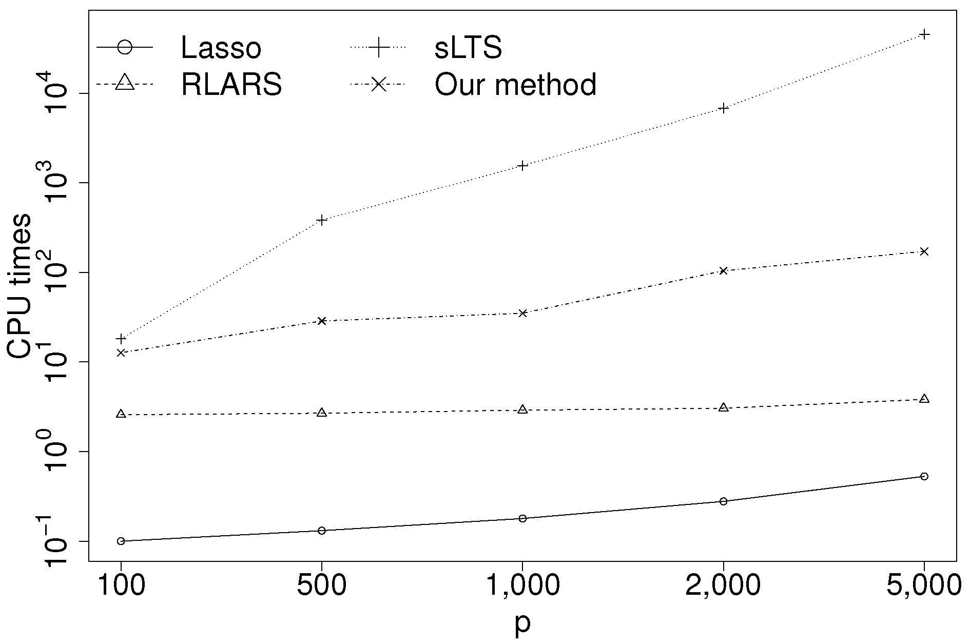
In this subsection, we consider the CPU times for Lasso, RLARS, sLTS and our method. The data were generated from the simulation model in Section 5.1. The sample size and the number of explanatory variables were set to be $n=100$ and $p=100,500,1000,2000,5000$, respectively. In Lasso, RLARS and sLTS, all parameters were used by default (see Section 5.3). Our method used the estimate of the RANSAC algorithm as an initial point. The number of candidates for the RANSAC algorithm was set to 1000. The parameters $\gamma$ and ${\gamma }_0$ were set to $0.1$ and $0.5$, respectively. No method used parallel computing methods. Figure 1 shows the average CPU times over 10 runs in seconds. All results were obtained in R Version 3.3.0 with an Intel Core i7-4790K machine. sLTS shows very high computational cost. RLARS is faster, but does not give a good estimate, as seen in Section 5.5. Our proposed method is fast enough even for $p=5000$.

Figure 1. CPU times (in seconds).

6. Real Data Analyses

In this section, we use two real datasets to compare our method with comparative methods in real data analysis. We show the best result of comparative methods among some parameter situations (e.g., Section 5.3).

6.1. NCI-60 Cancer Cell Panel

We applied our method and comparative methods to regress protein expression on gene expression data at the cancer cell panel of the National Cancer Institute. Experimental conditions were set in the same way as in Alfons et al. [4] as follows. The gene expression data were obtained with an Affymetrix HG-U133A chip and the normalized GCRMAmethod, resulting in a set of p = 22,283 explanatory variables. The protein expressions based on 162 antibodies were acquired via reverse-phase protein lysate arrays and ${log}_2$ transformed. One observation had to be removed since all values were missing in the gene expression data, reducing the number of observations to $n=59$. Then, the KRT18 antibody was selected as the response variable because it had the largest MAD among 162 antibodies, i.e., KRT18 may include a large number of outliers. Both the protein expressions and the gene expression data can be downloaded via the web application CellMiner (http://discover.nci.nih.gov/cellminer/). As a measure of prediction performance, the root trimmed mean squared prediction error (RTMSPE) was computed via leave-one-out cross-validation given by:

$$\begin{array}{c}\hfill \mathrm{RTMSPE}=\sqrt{\frac{1}{h}\sum _{i=1}^h{(e)}_{[i:n]}^2},\end{array}$$

where $e^2=({(y_1-x_1^T{\widehat{\beta }}^{[-1]})}^2,\dots ,{(y_n-x_n^T{\widehat{\beta }}^{[-n]})}^2)$ and ${(e)}_{[1:n]}^2\le \cdots \le {(e)}_{[n:n]}^2$ are the order statistics of $e^2$ and $h=\lfloor (n+1)0.75\rfloor$. The choice of h is important because it is preferable for estimating prediction performance that trimmed squares does not include outliers. We set h in the same way as in Alfons et al. [4], because the sLTS detected 13 outliers in Alfons et al. [4]. In this experiment, we used the estimate of the RANSAC algorithm as an initial point instead of sLTS because sLTS required high computational cost with such high dimensional data.

Table 6 shows that our method outperformed other comparative methods for the RTMSPE with high dimensional data. Our method presented the smallest RTMSPE with the second smallest number of explanatory variables. RLARS presented the smallest number of explanatory variables, but a much larger RTMSPE than our method.

Table 6. Root trimmed mean squared prediction error (RTMSPE) for protein expressions based on the KRT18 antibody (NCI-60 cancer cell panel data), computed from leave-one-out cross-validation.

Methods	RTMSPE	${}^1$ Selected Variables
Lasso	1.058	52
RLARS	0.936	18
sLTS	0.721	33
Our method ($\gamma =0.1$)	0.679	29
Our method ($\gamma =0.5$)	0.700	30

${}^1$ This means the number of non-zero elements.

6.2. Protein Homology Dataset

We applied our method and comparative methods to the protein sequence dataset used for KDD-Cup 2004. Experimental conditions were set in the same way as in Khan et al. [2] as follows. The whole dataset consists of $n=$ 145,751 protein sequences, which has 153 blocks corresponding to native protein. Each data point in a particular block is a candidate homologous protein. There were 75 variables in the dataset: the block number (categorical) and 74 measurements of protein features. The first protein feature was used as the response variable. Then, five blocks with a total of $n=4141$ protein sequences were selected because they contained the highest proportions of homologous proteins (and hence, the highest proportions of potential outliers). The data of each block were split into two almost equal parts to get a training sample of size $n_{tra}=2072$ and a test sample of size $n_{test}=2069$. The number of explanatory variables was $p=77$, consisting of four block indicators (Variables 1–4) and 73 features. The whole protein, training and test dataset can be downloaded from http://users.ugent.be/~svaelst/software/RLARS.html. As a measure of prediction performance, the root trimmed mean squared prediction error (RTMSPE) was computed for the test sample given by:

$$\begin{array}{c}\hfill \mathrm{RTMSPE}=\sqrt{\frac{1}{h}\sum _{i=1}^h{(e)}_{[i:n_{test}]}^2},\end{array}$$

where $e^2=({(y_1-{x_1}^T\widehat{\beta })}^2,\dots ,{(y_{n_{test}}-x_{n_{test}}^T\widehat{\beta })}^2)$ and ${(e)}_{[1:n_{test}]}^2\le \cdots \le {(e)}_{[n_{test}:n_{test}]}^2$ are the order statistics of $e^2$ and $h=\lfloor (n_{test}+1)0.99\rfloor ,\lfloor (n_{test}+1)0.95\rfloor \mathrm{or}\lfloor (n_{test}+1)0.9\rfloor$. In this experiment, we used the estimate of sLTS as an initial point.

Table 7 shows that our method outperformed other comparative methods for the RTMSPE. Our method presented the smallest RTMSPE with the largest number of explanatory variables. It might seem that other methods gave a smaller number of explanatory variables than necessary.

Table 7. Root trimmed mean squared prediction error in the protein test set.

	Trimming Fraction
Methods	1%	5%	10%	${}^{\mathbf{1}}$ Selected Variables
Lasso	10.697	9.66	8.729	22
RLARS	10.473	9.435	8.527	27
sLTS	10.614	9.52	8.575	21
Our method ($\gamma =0.1$)	10.461	9.403	8.481	44
Our method ($\gamma =0.5$)	10.463	9.369	8.419	42

${}^1$ This means the number of non-zero elements.

7. Conclusions

We proposed robust and sparse regression based on the $\gamma$-divergence. We showed desirable robust properties under both homogeneous and heterogeneous contamination. In particular, we presented the Pythagorean relation for the regression case, although it was not shown in Kanamori and Fujisawa [11]. In most of the robust and sparse regression methods, it is difficult to obtain the efficient estimation algorithm, because the objective function is non-convex and non-differentiable. Nonetheless, we succeeded to propose the efficient estimation algorithm, which has a monotone decreasing property of the objective function by using the MM-algorithm. The numerical experiments and real data analyses suggested that our method was superior to comparative robust and sparse linear regression methods in terms of both accuracy and computational costs. However, in numerical experiments, a few results of performance measure “TNR” were a little less than the best results. Therefore, if more sparsity of coefficients is needed, other sparse penalties, e.g., the Smoothly Clipped Absolute Deviations (SCAD) [22] and the Minimax Concave Penalty (MCP) [23], can also be useful.

References

- Tibshirani, R. Regression shrinkage and selection via the lasso. J. R. Stat. Soc. Ser. B 1996, 58, 267–288. [Google Scholar]
- Khan, J.A.; Van Aelst, S.; Zamar, R.H. Robust linear model selection based on least angle regression. J. Am. Stat. Assoc. 2007, 102, 1289–1299. [Google Scholar] [CrossRef]
- Efron, B.; Hastie, T.; Johnstone, I.; Tibshirani, R. Least angle regression. Ann. Stat. 2004, 32, 407–499. [Google Scholar]
- Alfons, A.; Croux, C.; Gelper, S. Sparse least trimmed squares regression for analyzing high-dimensional large data sets. Ann. Appl. Stat. 2013, 7, 226–248. [Google Scholar] [CrossRef]
- Rousseeuw, P.J. Least Median of Squares Regression. J. Am. Stat. Assoc. 1984, 79, 871–880. [Google Scholar] [CrossRef]
- Windham, M.P. Robustifying model fitting. J. R. Stat. Soc. Ser. B 1995, 57, 599–609. [Google Scholar]
- Basu, A.; Harris, I.R.; Hjort, N.L.; Jones, M.C. Robust and efficient estimation by minimising a density power divergence. Biometrika 1998, 85, 549–559. [Google Scholar] [CrossRef]
- Jones, M.C.; Hjort, N.L.; Harris, I.R.; Basu, A. A Comparison of related density-based minimum divergence estimators. Biometrika 2001, 88, 865–873. [Google Scholar] [CrossRef]
- Fujisawa, H.; Eguchi, S. Robust Parameter Estimation with a Small Bias Against Heavy Contamination. J. Multivar. Anal. 2008, 99, 2053–2081. [Google Scholar] [CrossRef]
- Basu, A.; Shioya, H.; Park, C. Statistical Inference: The Minimum Distance Approach; CRC Press: Boca Raton, FL, USA, 2011. [Google Scholar]
- Kanamori, T.; Fujisawa, H. Robust estimation under heavy contamination using unnormalized models. Biometrika 2015, 102, 559–572. [Google Scholar] [CrossRef]
- Cichocki, A.; Cruces, S.; Amari, S.I. Generalized Alpha-Beta Divergences and Their Application to Robust Nonnegative Matrix Factorization. Entropy 2011, 13, 134–170. [Google Scholar] [CrossRef]
- Samek, W.; Blythe, D.; Müller, K.R.; Kawanabe, M. Robust Spatial Filtering with Beta Divergence. In Advances in Neural Information Processing Systems 26; Burges, C.J.C., Bottou, L., Welling, M., Ghahramani, Z., Weinberger, K.Q., Eds.; Curran Associates, Inc.: Red Hook, NY, USA, 2013; pp. 1007–1015. [Google Scholar]
- Hunter, D.R.; Lange, K. A tutorial on MM algorithms. Am. Stat. 2004, 58, 30–37. [Google Scholar] [CrossRef]
- Hirose, K.; Fujisawa, H. Robust sparse Gaussian graphical modeling. J. Multivar. Anal. 2017, 161, 172–190. [Google Scholar] [CrossRef]
- Zou, H.; Hastie, T. Regularization and variable selection via the Elastic Net. J. R. Stat. Soc. Ser. B 2005, 67, 301–320. [Google Scholar] [CrossRef]
- Yuan, M.; Lin, Y. Model selection and estimation in regression with grouped variables. J. R. Stat. Soc. Ser. B 2006, 68, 49–67. [Google Scholar] [CrossRef]
- Tibshirani, R.; Saunders, M.; Rosset, S.; Zhu, J.; Knight, K. Sparsity and smoothness via the fused lasso. J. R. Stat. Soc. Ser. B 2005, 67, 91–108. [Google Scholar] [CrossRef]
- Friedman, J.; Hastie, T.; Höfling, H.; Tibshirani, R. Pathwise coordinate optimization. Ann. Appl. Stat. 2007, 1, 302–332. [Google Scholar] [CrossRef]
- Hastie, T.; Tibshirani, R.; Friedman, J. The Elements of Statistical Learning: Data Mining, Inference and Prediction; Springer: New York, NY, USA, 2010. [Google Scholar]
- Maronna, R.A.; Martin, D.R.; Yohai, V.J. Robust Statistics: Theory and Methods; John Wiley and Sons: Hoboken, NJ, USA, 2006. [Google Scholar]
- Fan, J.; Li, R. Variable Selection via Nonconcave Penalized Likelihood and its Oracle Properties. J. Am. Stat. Assoc. 2001, 96, 1348–1360. [Google Scholar]
- Zhang, C.H. Nearly unbiased variable selection under minimax concave penalty. Ann. Stat. 2010, 38, 894–942. [Google Scholar] [CrossRef]
© 2017 by the authors. Licensee MDPI, Basel, Switzerland. This article is an open access article distributed under the terms and conditions of the Creative Commons Attribution (CC BY) license (http://creativecommons.org/licenses/by/4.0/).