Reliable Approximation of Long Relaxation Timescales in Molecular Dynamics

Abstract

Many interesting rare events in molecular systems, like ligand association, protein folding or conformational changes, occur on timescales that often are not accessible by direct numerical simulation. Therefore, rare event approximation approaches like interface sampling, Markov state model building, or advanced reaction coordinate-based free energy estimation have attracted huge attention recently. In this article we analyze the reliability of such approaches. How precise is an estimate of long relaxation timescales of molecular systems resulting from various forms of rare event approximation methods? Our results give a theoretical answer to this question by relating it with the transfer operator approach to molecular dynamics. By doing so we also allow for understanding deep connections between the different approaches.

1. Introduction

The problem of accurate estimation of long relaxation timescales associated with rare events in molecular dynamics like ligand association, protein folding, or conformational changes has attracted a lot of attention recently. Often, these timescales are not accessible by direct numerical simulation. Therefore, different discrete coarse graining approaches for their approximation, like Markov state model (MSM) building [1,2] or time-lagged independent component analysis (TiCA) [3,4] have been introduced and successfully applied to various molecular systems [5,6]. These approaches are based on finite-dimensional Galerkin discretization [1] or variational approximation [7,8] of the transfer operator of the molecular dynamics process [9]. In several theoretical studies the approximation error of these numerical techniques regarding the longest relaxation timescales has been analyzed resulting in error estimates in terms of the dominant eigenvalues of the transfer operator [3,9]. In this article we first show how to obtain similar error estimates when replacing the transfer operator by the infinitesimal generator [10] associated with it. Furthermore, the analysis exhibits that the different approaches are deeply connected, that is, in the end they lead to an identical numerical problem. In addition to the different discrete coarse graining approaches, the literature contains various alternative reaction coordinate sampling approaches aiming at approximation of very long relaxation processes. In these sampling approaches, one assumes that the effective dynamical behavior of the systems on long timescales can be described by a relatively low dimensional object given by some reaction coordinates. Various advanced methods such as umbrella sampling [11,12], metadynamics [13,14], blue moon sampling [15], the adaptive biasing force method [16], or temperature-accelerated molecular dynamics (TAMD) [17], as well as trajectory-based techniques like milestoning [18], transition interface sampling [19], or forward flux sampling [20] may serve as some examples. These methods result in free energy barriers, transition rates, or first mean passage times for the rare events of interest; they are complemented by several approaches to the effective dynamics of the reaction coordinate space [21,22,23] that allow for significantly faster simulation of these rare events [24,25,26] including details of the underlying molecular mechanisms. Surprisingly, our analytic tools, originally developed for discrete coarse graining approaches, can also be utilized for evaluating the approximation quality of reaction coordinate sampling approaches to the effective dynamics. We derive an explicit error estimate for the longest timescale resulting from the choice of specific reaction coordinates.

However, estimating the approximation quality is not the only way of utilizing the analytical insights presented in this article. We also demonstrate how the new techniques for simulation of the effective dynamics can be used for efficient MSM building or TiCA applications.

Mathematically, the article is based on the analysis of the dominant timescales of reversible and ergodic diffusion processes in energy landscapes. The leading eigenvalues of the transfer operator (or, equivalently, the infinitesimal generator) and the corresponding eigenfunctions characterize the dynamical behavior of the process on long timescales [9,27]. Firstly, in several articles the approximation error with respect to these leading eigenvalues under discretization of the transfer operator has been discussed, cf. [3,7,8,28,29,30]. Following this work, we characterize the approximation quality for the (low-lying) eigenvalues of the infinitesimal generator. This permits us to study the connection between the effective dynamics considered in [23] and Galerkin discretization schemes for the transfer operator. Secondly, following the work [7,8], we study the variational approach for the infinitesimal generator. In fact, we will see that this approach leads to the same generalized matrix eigenproblem as the one resulting from Galerkin discretization. Thirdly, numerical issues related to the estimation of the coefficient matrices by means of the effective dynamics are discussed.

The paper is organized as follows. In Section 2, we introduce the various operators associated to the reversible diffusion processes and discuss the relation between eigenvalues and relaxation timescales. Next, in Section 3, we study the Galerkin discretization of generators/transfer operators for solving the eigenproblem and show that previous results can be extended to reaction coordinate subspaces. In Section 4, the variational approach to the approximation of the eigenproblem is considered and its relations to the Galerkin approach are worked out in detail. Then, in Section 5, we discuss numerical issues related to estimating the discretization matrices by means of simulating the effective dynamics for given reaction coordinates; the performance of this approach is studied numerically in Section 6. Finally, conclusions and some further remarks are given in Section 7. After being familiar with the facts in Section 2, readers who are more interested in numerical algorithmic aspects rather than detailed mathematical analysis can skip Section 3 and Section 4 and refer to Section 5 and Section 6 on first reading.

2. Diffusion Process and the Associated Operators

We consider a diffusion process given by the stochastic differential equation (SDE)

$$\begin{array}{cc}\hfill d{x}_s& =-\nabla V(x_s)ds+\sqrt{2{\beta }^{-1}}d{w}_s,s\ge 0,\hfill \\ \hfill x_0& =x,\hfill \end{array}$$

(1)

where $x_s\in {\mathbb{R}}^n$, parameter $\beta >0$ is related to the inverse of system’s temperature, and $w_s$ is an n-dimensional Brownian motion. $V:{\mathbb{R}}^n\to \mathbb{R}$ is a potential function which is assumed to be smooth and bounded from below. The results presented subsequently can be extended to more general reversible diffusion processes with a state-dependent noise intensity matrix, cf. [23]. However, for the sake of simplicity of presentation we restrict our considerations to the specific case (1) typically studied in molecular dynamics.

The infinitesimal generator of the dynamics (1) is given by,

$$\begin{array}{c}\hfill \mathcal{L}=-\nabla V·\nabla +\frac{1}{\beta }\mathrm{\Delta }.\end{array}$$

(2)

It is known that, under mild conditions on V, the solution process ${(x_s)}_{s\ge 0}$ of (1) is ergodic [31], and its unique invariant measure $\pi$ is given by $\pi (dx)=\rho (x)dx$ where,

$$\begin{array}{c}\hfill \rho (x)=\frac{1}{Z}{e}^{-\beta V(x)},\mathrm{with}Z={\int }_{{\mathbb{R}}^n}{e}^{-\beta V(x)}dx.\end{array}$$

(3)

We introduce the Hilbert space $H=L^2({\mathbb{R}}^n,\pi )$, which is endowed with the inner product,

$$\begin{array}{c}\hfill {⟨f,g⟩}_{\pi }={\int }_{{\mathbb{R}}^n}f(x)g(x)\rho (x)dx,\forall f,g\in H,\end{array}$$

(4)

and the norm ${|f|}_{\pi }=\sqrt{{⟨f,f⟩}_{\pi }}$ , $\forall f\in H$. The domain of the operator $\mathcal{L}$ will be denoted as $D(\mathcal{L})\subset H$.

It is also known that the process ${(x_s)}_{s\ge 0}$ is a reversible process and that $\mathcal{L}$ is a self-adjoint operator with respect to the inner product (4). Whenever the potential V grows to infinity fast enough at infinity, its spectrum is discrete [9]. Let ${\lambda }_i\in \mathbb{C}$ and ${\phi }_i\in D(\mathcal{L})$ be the eigenvalues and the corresponding (normalized) eigenfunctions of $-\mathcal{L}$, that is, the solutions of the eigenproblem,

$$\begin{array}{c}\hfill -\mathcal{L}f=\lambda f\end{array}$$

(5)

in H, or in weak form,

$$\begin{array}{c}\hfill -{⟨\mathcal{L}f,g⟩}_{\pi }=\lambda {⟨f,g⟩}_{\pi },\forall g\in H.\end{array}$$

(6)

Due to the self-adjointness of $\mathcal{L}$ and the fact that,

$$\begin{array}{c}\hfill {⟨-\mathcal{L}f,f⟩}_{\pi }=\frac{1}{\beta }{\int }_{{\mathbb{R}}^n}{|\nabla f(x)|}^2\rho (x)dx\ge 0,\forall f\in H,\end{array}$$

(7)

we can assume that ${\lambda }_i\in \mathbb{R}$ with,

$$\begin{array}{c}\hfill 0={\lambda }_0<{\lambda }_1\le \cdots \le {\lambda }_k\le \cdots ,\end{array}$$

(8)

with ${\phi }_0\equiv 1$.

Given $s\ge 0$, we define the operator $T_s:H\to H$ by,

$$\begin{array}{c}\hfill (T_{s}f)(x)=\mathbf{E}\left(f(x_s)|x_0=x\right),f\in H,\end{array}$$

(9)

where $\mathbf{E}$ denotes the expectation taken with respect to the paths of (1) under the initial condition that $x_0=x$. It is well-known that $u(s,x)=T_{s}f(x)$ is the solution of the Kolmogorov backward equation

$$\frac{d}{ds}u(s,·)=\mathcal{L}u(s,·),u(0,·)=f,$$

(10)

that is, the operators $T_s$, $s\ge 0$ form a one-parameter semigroup whose infinitesimal generator is $\mathcal{L}$, and therefore they are self-adjoint in H as well. Because of Equation (10), the formal expression $T_s=e^{s\mathcal{L}}$ is often used in the literature. Similarly to (8), we also know that the eigenvalues of $T_s$ are given by,

$$\begin{array}{c}\hfill 1=e^{-{\lambda }_{0}s}>e^{-{\lambda }_{1}s}\ge \cdots >0,\end{array}$$

(11)

with the same eigenfunctions ${\phi }_i$, $i=0,1,\cdots$.

In the following we introduce another operator called the transfer operator, which has been extensively considered in the literature, to investigate the metastability of molecular systems and to build Markov state models (MSM) [1,6,9]. A lag time $\tau >0$ is fixed, with $p(x,·;\tau )$ being the transition density function of the process (1) starting from $x\in {\mathbb{R}}^n$, i.e., $p(x,y;\tau )$ describes the probability density of starting from state x at time $s=0$ and arriving at $y\in {\mathbb{R}}^n$ after time $\tau$. For a bounded and continuous function $u\in H$, the transfer operator ${\mathcal{T}}_{\tau }:H\to H$ is defined by [1,27,32],

$$\begin{array}{c}\hfill ({\mathcal{T}}_{\tau }u)(y)=\frac{1}{\rho (y)}{\int }_{{\mathbb{R}}^n}p(x,y;\tau )u(x)\rho (x)dx,y\in {\mathbb{R}}^n.\end{array}$$

(12)

From (12), it follows immediately that,

$$\begin{array}{cc}\hfill {⟨{\mathcal{T}}_{\tau }u,f⟩}_{\pi }=& {\int }_{{\mathbb{R}}^n}{\int }_{{\mathbb{R}}^n}p(x,y;\tau )f(y)dyu(x)\rho (x)dx\hfill \\ \hfill =& {\int }_{{\mathbb{R}}^n}\left[\mathbf{E}\left(f(x_{\tau })|x_0=x\right)\right]u(x)\rho (x)dx\hfill \\ \hfill =& {⟨u,T_{\tau }f⟩}_{\pi }={⟨T_{\tau }u,f⟩}_{\pi },\forall f\in H,\hfill \end{array}$$

which then implies ${\mathcal{T}}_{\tau }=T_{\tau }$, i.e., the transfer operator ${\mathcal{T}}_{\tau }$ coincides with the operator $T_{\tau }$, a member within the semigroup ${(T_s)}_{s\ge 0}$. Denote the eigenvalues of ${\mathcal{T}}_{\tau }$ as ${\mu }_i$, $i\ge 0$, such that,

$$\begin{array}{c}\hfill 1={\mu }_0>{\mu }_1\ge \cdots >0.\end{array}$$

(13)

Then from the discussions above and the eigenvalues of $T_s$ in (11), we can conclude that ${\mu }_i=e^{-{\lambda }_i\tau }$ and the corresponding eigenfunctions are the same as the eigenfunctions ${\phi }_i$ of the infinitesimal generator $\mathcal{L}$. These eigenvalues and eigenfunctions encode crucial timescale information of the dynamical system. Specifically, the relaxation timescales $t_i$ of the dynamics (1) are given by [10],

$$t_i={\lambda }_i^{-1},i=1,2,\dots .$$

This means that the dominant relaxation timescales of the dynamics (1) can be obtained by computing the dominant eigenvalues of ${\mathcal{T}}_{\tau }$ (or, equivalently, $T_{\tau }$, $\mathcal{L}$), cf. [10,27].

3. Galerkin Approximation of the Eigenvalues of the Generator

In this section, we study the Galerkin method for computing the eigenvalues of the infinitesimal generator $\mathcal{L}$. While Galerkin discretization of the transfer operator has been studied to some extent [9], results on the associated infinitesimal generator are rather sparse.

3.1. Some General Results

To introduce the Galerkin method, let $H_0$ be a Hilbert subspace of H containing the constant function, and let $\mathbf{P}$ denote the orthogonal projection operator from H to $H_0$, which satisfies ${\mathbf{P}}^2=\mathbf{P}$ and,

$$\begin{array}{c}\hfill {⟨\mathbf{P}f,g⟩}_{\pi }={⟨f,g⟩}_{\pi },\forall f\in H,g\in H_0.\end{array}$$

(14)

The Galerkin method aims at approximating the solution of (6) in the subspace $H_0$. Specifically, we want to find $f\in H_0$, such that,

$$\begin{array}{c}\hfill -{⟨\mathcal{L}f,g⟩}_{\pi }=\kappa {⟨f,g⟩}_{\pi },\forall g\in H_0,\end{array}$$

(15)

for some constant $\kappa \ge 0$. Using the property (14), we know that problem (15) is equivalent to the eigenproblem for the operator $-\mathbf{P}\mathcal{L}$ on the subspace $H_0$, i.e.,

$$\begin{array}{c}\hfill -\mathbf{P}\mathcal{L}f=\kappa f.\end{array}$$

(16)

It is straightforward to verify that $-\mathbf{P}\mathcal{L}$ is a self-adjoint operator on $H_0$. Similarly to (8), let ${\zeta }_i\in H_0$ be the orthonormal eigenfunctions of the operator $-\mathbf{P}\mathcal{L}$ corresponding to eigenvalues ${\kappa }_i$, where,

$$\begin{array}{c}\hfill 0={\kappa }_0<{\kappa }_1\le {\kappa }_2\le \cdots ,\end{array}$$

(17)

and ${\zeta }_0\equiv 1$. When $H_0$ is an infinite dimensional subspace, we assume ${\kappa }_i\to +\infty$ as $i\to +\infty$.

In the following, we want to study the condition under which the eigenvalues of the projected generator $\mathbf{P}\mathcal{L}$ are reliable approximations of the eigenvalues of the full generator $\mathcal{L}$. The following approximation result was obtained in [23] and we include its proof for completeness:

Theorem 1.

For $i\ge 0$, let ${\phi }_i$ and ${\zeta }_i$ be the orthonormal eigenfunctions of the operators $-\mathcal{L}$ and $-\mathbf{P}\mathcal{L}$ corresponding to the eigenvalues ${\lambda }_i$ and ${\kappa }_i$, respectively. We have,

$$\begin{array}{c}\hfill {\lambda }_i\le {\kappa }_i\le {\lambda }_i+\frac{1}{\beta }{\int }_{{\mathbb{R}}^n}|\nabla ({\phi }_i-{\zeta }_i)(x){|}^2\rho (x)dx.\end{array}$$

(18)

Proof. 

From (15), we have ${\kappa }_i=-{⟨\mathcal{L}{\zeta }_i,{\zeta }_i⟩}_{\pi }$. Define the subspace $E_{i+1}=span\{{\zeta }_0,\dots ,{\zeta }_i\}$ for $i\ge 0$. It follows from the orthogonality of the functions ${\zeta }_i$ that $E_{i+1}$ is an $(i+1)$-dimensional subspace of H. Using (17) it is direct to verify that,

$$\begin{array}{c}\hfill {\kappa }_i=\underset{f\in E_{i+1},{|f|}_{\pi }=1}{\max }{⟨-\mathcal{L}f,f⟩}_{\pi }.\end{array}$$

(19)

Applying the min–max theorem to the eigenvalues of the operator $-\mathcal{L}$, we conclude,

$$\begin{array}{c}\hfill {\kappa }_i=\underset{f\in E_{i+1},{|f|}_{\pi }=1}{\max }{⟨-\mathcal{L}f,f⟩}_{\pi }\ge \underset{E_{i+1}^{\prime }}{\min }\underset{f\in E_{i+1}^{\prime },{|f|}_{\pi }=1}{\max }{⟨-\mathcal{L}f,f⟩}_{\pi }={\lambda }_i,\end{array}$$

(20)

where $E_{i+1}^{\prime }$ goes over all $(i+1)$-dimensional subspaces of H. For the upper bound, we can compute that,

$$\begin{array}{c}\hspace{1em}{⟨-\mathcal{L}({\phi }_i-{\zeta }_i),({\phi }_i-{\zeta }_i)⟩}_{\pi }\hfill \\ ={⟨-\mathcal{L}{\phi }_i,{\phi }_i⟩}_{\pi }+2{⟨\mathcal{L}{\phi }_i,{\zeta }_i⟩}_{\pi }+{⟨-\mathcal{L}{\zeta }_i,{\zeta }_i⟩}_{\pi }\hfill \\ ={\lambda }_i-2{\lambda }_i{⟨{\phi }_i,{\zeta }_i⟩}_{\pi }+{\kappa }_i\hfill \\ ={\kappa }_i-{\lambda }_i+2{\lambda }_i\left(1-{⟨{\phi }_i,{\zeta }_i⟩}_{\pi }\right)\ge {\kappa }_i-{\lambda }_i,\hfill \end{array}$$

where we have used the fact that ${⟨{\phi }_i,{\zeta }_i⟩}_{\pi }\le |{\phi }_i{|}_{\pi }{|{\zeta }_i|}_{\pi }=1$. The conclusion follows from (7). ☐

Previous studies on the Galerkin approximation of the dominant eigenvalues of the transfer operator have shown that the approximation error of eigenvalues can be reliably bounded by means of the projection errors of the corresponding eigenfunctions [28,29,30]. Next we will derive a similar result for the generator $\mathcal{L}$. To this end, we introduce the orthogonal projection ${\mathbf{P}}^{\perp }$ from H to the complement subspace $H_0^{\perp }$ of $H_0$, that is, ${\mathbf{P}}^{\perp }=\mathbf{I}-\mathbf{P}$. We have

Theorem 2.

Let φ be a normalized eigenfunction of the operator $-\mathcal{L}$ corresponding to the eigenvalue λ. Define constants,

$$\begin{array}{c}\hfill {\delta }_1=|\mathcal{L}{\mathbf{P}}^{\perp }{\phi |}_{\pi },{\delta }_2={|{\mathbf{P}}^{\perp }\phi |}_{\pi }\le 1,\end{array}$$

(21)

and suppose that $0<{\delta }_2<1$. Then there is an eigenvalue ${\kappa }_i$ of the operator $-\mathbf{P}\mathcal{L}$, such that,

$$\begin{array}{c}\hfill |{\kappa }_i-\lambda |\le \frac{{\delta }_1}{{(1-{\delta }_2^2)}^{\frac{1}{2}}}.\end{array}$$

(22)

Proof. 

Since ${\delta }_2={|{\mathbf{P}}^{\perp }\phi |}_{\pi }={\left(1-{|\mathbf{P}\phi |}_{\pi }^2\right)}^{\frac{1}{2}}<1$, we have $|\mathbf{P}\phi |>0$. Let $\mathbf{P}\phi ={\displaystyle \sum _{i=0}^{+\infty }}{\omega }_i{\zeta }_i$, where ${\omega }_i={⟨\phi ,{\zeta }_i⟩}_{\pi }$, and the summation consists of finite terms when $H_0$ is a finite dimensional subspace. For all $g\in H_0$, we can compute,

$$\begin{array}{c}\hspace{1em}{⟨\mathbf{P}\mathcal{L}{\mathbf{P}}^{\perp }\phi ,g⟩}_{\pi }={⟨\mathbf{P}\mathcal{L}(\phi -\mathbf{P}\phi ),g⟩}_{\pi }\hfill \\ ={⟨\mathbf{P}\mathcal{L}\phi ,g⟩}_{\pi }-⟨\mathbf{P}\mathcal{L}\left(\sum _{i=0}^{+\infty }{\omega }_i{\zeta }_i\right),g{⟩}_{\pi }\hfill \\ =-{⟨\lambda \mathbf{P}\phi ,g⟩}_{\pi }+{⟨\sum _{i=0}^{+\infty }{\omega }_i{\kappa }_i{\zeta }_i,g⟩}_{\pi }=⟨\sum _{i=0}^{+\infty }{\omega }_i({\kappa }_i-\lambda ){\zeta }_i,g{⟩}_{\pi },\hfill \end{array}$$

which implies $\mathbf{P}\mathcal{L}{\mathbf{P}}^{\perp }\phi =\sum _{i=0}^{+\infty }{\omega }_i({\kappa }_i-\lambda ){\zeta }_i$, and,

$$\begin{array}{c}\hfill |\mathbf{P}\mathcal{L}{\mathbf{P}}^{\perp }{\phi |}_{\pi }^2=\sum _{i=0}^{+\infty }{\omega }_i^2|{\kappa }_i{-\lambda |}^2\ge \left(\underset{i}{\min }{|{\kappa }_i-\lambda |}^2\right)\sum _{i=0}^{+\infty }{\omega }_i^2=\underset{i}{\min }|{\kappa }_i{-\lambda |}^2{|\mathbf{P}\phi |}_{\pi }^2.\end{array}$$

Therefore we have,

$$\begin{array}{c}\hfill \underset{i}{\min }|{\kappa }_i-\lambda |\le \frac{|\mathbf{P}\mathcal{L}{\mathbf{P}}^{\perp }{\phi |}_{\pi }}{{|\mathbf{P}\phi |}_{\pi }}\le \frac{|\mathcal{L}{\mathbf{P}}^{\perp }{\phi |}_{\pi }}{{\left(1-|{\mathbf{P}}^{\perp }{\phi |}_{\pi }^2\right)}^{\frac{1}{2}}}=\frac{{\delta }_1}{{(1-{\delta }_2^2)}^{\frac{1}{2}}}.\end{array}$$

(23)

☐

Remark 1.

Notice that our error bound above relies on both constants ${\delta }_1$ and ${\delta }_2$, while the error bound in [30] for the transfer operator only depends on one constant, the projection error ${\delta }_2$. This difference is due to the fact that the generator $\mathcal{L}$ is an unbounded operator while the transfer operator is bounded.

3.2. Finite Dimensional Subspaces

In applications, it is often assumed that $H_0$ is spanned by finitely many basis functions. In particular, this is the situation when constructing MSMs based on indicator functions of partition sets [30] or based on core sets [10].

Let $H_0$ be the finite dimensional space $H_0=span\{{\psi }_1,{\psi }_2,\cdots ,{\psi }_N\}$, where ${\psi }_i\in H$ are the basis functions, and consider the eigenproblem (15). As a direct application of Theorem 1 and Theorem 2, we have,

Corollary 1.

For Galerkin approximation of the eigenproblem (15) using the finite-dimensional ansatz space $H_0$, the following three statements are valid:

1. 

Write $f=\sum _{i=1}^N{\omega }_i{\psi }_i\in H_0$ and let $X={({\omega }_1,{\omega }_2,\cdots ,{\omega }_N)}^T\in {\mathbb{R}}^N$. Then problem (15) is equivalent to the generalized matrix eigenproblem,

$$\begin{array}{c}\hfill CX=\lambda SX,\end{array}$$

(24)

where $C,S$ are $N\times N$ matrices whose entries are given by,

$$\begin{array}{c}\hfill C_{l{l}^{\prime }}={⟨-\mathcal{L}{\psi }_l,{\psi }_{l^{\prime }}⟩}_{\pi },S_{l{l}^{\prime }}={⟨{\psi }_l,{\psi }_{l^{\prime }}⟩}_{\pi },1\le l,l^{\prime }\le N,\end{array}$$

(25)

2. 

Let $0={\kappa }_0\le {\kappa }_1\le \cdots \le {\kappa }_k$ be the $(k+1)$ smallest eigenvalues of problem (24) and,

$$\begin{array}{c}\hfill X_i={(X_{i1},X_{i2},\cdots ,X_{iN})}^T,0\le i\le k,\end{array}$$

be the orthonormal eigenvector corresponding to ${\kappa }_i$ such that $X_i^{T}S{X}_i=1$. Define ${\zeta }_i={\displaystyle \sum _{l=1}^N}{X}_{il}{\psi }_l$, then we have,

$$\begin{array}{c}\hfill {\lambda }_i\le {\kappa }_i\le {\lambda }_i+\frac{1}{\beta }{\int }_{{\mathbb{R}}^n}{|\nabla ({\phi }_i-{\zeta }_i)(x)|}^2\rho (x)dx,0\le i\le k,\end{array}$$

(26)

where ${\lambda }_i$, ${\phi }_i$ are the eigenvalues and the eigenfunctions of the operator $-\mathcal{L}$, respectively.

3. 

Let $\mathbf{P}$ be the orthogonal projection operator from H to $H_0$, and φ be an eigenfunction of the operator $-\mathcal{L}$ corresponding to the eigenvalue λ. Define constants,

$$\begin{array}{c}\hfill {\delta }_1=|\mathcal{L}{\mathbf{P}}^{\perp }{\phi |}_{\pi },{\delta }_2={|{\mathbf{P}}^{\perp }\phi |}_{\pi },\end{array}$$

and suppose that ${\delta }_2<1$. Then there is an eigenvalue ${\kappa }_i$ of problem (24) such that,

$$\begin{array}{c}\hfill |{\kappa }_i-\lambda |\le \frac{{\delta }_1}{{(1-{\delta }_2^2)}^{\frac{1}{2}}}.\end{array}$$

(27)

3.3. Infinite Dimensional Subspace: Effective Dynamics

In this subsection, we discuss Galerkin approximations based on infinite-dimensional ansatz spaces; these cases appear when studying the effective dynamics given by a so-called reaction coordinate, cf. [23]. In order to explain the relation between Galerkin approximation and effective dynamics, let us first recall some definitions and results regarding the effective dynamics. For more details, readers are referred to [21,23,33] for related work.

Let $\xi :{\mathbb{R}}^n\to {\mathbb{R}}^m$ be a reaction coordinate function, $m\ge 1$. For any function $f\in H$ and $x\in {\mathbb{R}}^n$, we define,

$$\begin{array}{c}\hfill \begin{array}{cc}\hfill \mathbf{P}f(x)=& \frac{1}{Q(z)}{\int }_{{\mathbb{R}}^n}\rho (x^{\prime })f(x^{\prime })\delta \left(\xi (x^{\prime })-z\right)d{x}^{\prime },\hfill \end{array}\end{array}$$

(28)

where $z=\xi (x)\in {\mathbb{R}}^m$, $\delta (·)$ denotes the delta function, and $Q(z)={\int }_{{\mathbb{R}}^n}\rho (x^{\prime })\delta \left(\xi (x^{\prime })-z\right)d{x}^{\prime }$ is a normalization factor satisfying ${\int }_{{\mathbb{R}}^m}Q(z)dz=1$. Define the probability measure $\nu$ on ${\mathbb{R}}^m$ given by $\nu (dz)=Q(z)dz$ for $z\in {\mathbb{R}}^m$ and consider the Hilbert space $\tilde{H}=L^2({\mathbb{R}}^m,\nu )$. $\tilde{H}$ induces a (infinite dimensional) linear subspace of H, namely,

$$\begin{array}{c}\hfill H_0=\left\{f|f\in H,f=\tilde{f}\circ \xi ,\mathrm{for} \mathrm{some}\tilde{f}\in \tilde{H}\right\}\subset H,\end{array}$$

(29)

and (28) clearly implies that $\mathbf{P}f\in H_0$.

Let $\tilde{f}\in \tilde{H}$ satisfy $\mathbf{P}f=\tilde{f}\circ \xi$. Then, using (28), we can verify that ${\mathbf{P}}^2=\mathbf{P}$ and,

$$\begin{array}{c}\hfill {⟨f,h⟩}_{\pi }={⟨\mathbf{P}f,h⟩}_{\pi }={⟨\tilde{f},\tilde{h}⟩}_{\nu },\forall h=\tilde{h}\circ \xi \in H_0.\end{array}$$

(30)

Therefore, the mapping $\mathbf{P}:H\to H_0$ actually is the orthogonal projection operator from H to the subspace $H_0$. For $f\in H$, $z\in {\mathbb{R}}^m$, in the following we will also write $\mathbf{P}f(z)$ instead of $\tilde{f}(z)$, where $\tilde{f}\in \tilde{H}$ such that $\mathbf{P}f=\tilde{f}\circ \xi$. The effective dynamics of the dynamics (1) for the reaction coordinate $\xi$ is defined on ${\mathbb{R}}^m$ and satisfies the SDE,

$$\begin{array}{c}\hfill d{z}_s=\tilde{b}(z_s)ds+\sqrt{2{\beta }^{-1}}\tilde{\sigma }(z_s)d{w}_s,\end{array}$$

(31)

where $z_s\in {\mathbb{R}}^m$, $w_s$ is a Brownian motion on ${\mathbb{R}}^m$, and the coefficients $\tilde{b}:{\mathbb{R}}^m\to {\mathbb{R}}^m$, $\tilde{\sigma }:{\mathbb{R}}^m\to {\mathbb{R}}^{m\times m}$ are given by,

$$\begin{array}{c}\hfill \begin{array}{cc}\hfill {\tilde{b}}_l(z)=& \mathbf{P}(\mathcal{L}{\xi }_l)(z)=\mathbf{P}\left(-\nabla V·\nabla {\xi }_l+\frac{1}{\beta }\mathrm{\Delta }{\xi }_l\right)(z),\hfill \\ \hfill {\tilde{a}}_{l{l}^{\prime }}(z)=& {(\tilde{\sigma }{\tilde{\sigma }}^T)}_{l{l}^{\prime }}(z)=\mathbf{P}\left(\sum _{i=1}^n\frac{\partial {\xi }_l}{\partial x_i}\frac{\partial {\xi }_{l^{\prime }}}{\partial x_i}\right)(z),\hfill \end{array}\end{array}$$

(32)

for $\forall z\in {\mathbb{R}}^m$, $1\le l,l^{\prime }\le m$. The infinitesimal generator of the process governed by (31) is given by,

$$\begin{array}{cc}\hfill \tilde{\mathcal{L}}=& \sum _{l=1}^m{\tilde{b}}_l\frac{\partial }{\partial z_l}+\frac{1}{\beta }\sum _{l,l^{\prime }=1}^m{\tilde{a}}_{l{l}^{\prime }}\frac{{\partial }^2}{\partial z_l\partial z_{l^{\prime }}},\hfill \end{array}$$

(33)

which is a self-adjoint operator on space $\tilde{H}$ with discrete spectrum under appropriate conditions on $\xi$. We consider the eigenproblem,

$$\begin{array}{c}\hfill -\tilde{\mathcal{L}}\tilde{f}=\tilde{\lambda }\tilde{f},\tilde{f}\in \tilde{H},\end{array}$$

(34)

and let ${\tilde{\phi }}_i\in \tilde{H}$ be the orthonormal eigenfunctions of the operator $-\tilde{\mathcal{L}}$ corresponding to the eigenvalues ${\tilde{\lambda }}_i$, where,

$$\begin{array}{c}\hfill 0={\tilde{\lambda }}_0<{\tilde{\lambda }}_1\le {\tilde{\lambda }}_2\le \cdots .\end{array}$$

(35)

Applying Theorems 1 and 2, we have the following result.

Corollary 2.

For the eigenproblem (34) associated with the effective dynamics, the following three statements are valid:

1. 

For $f=\tilde{f}\circ \xi \in H_0$ where $\tilde{f}\in \tilde{H}$, we have,

$$\begin{array}{c}\hfill \mathbf{P}\mathcal{L}f=\left(\tilde{\mathcal{L}}\tilde{f}\right)\circ \xi .\end{array}$$

(36)

2. 

Let ${\phi }_i$ and ${\tilde{\phi }}_i$ be the normalized eigenfunctions of the operators $-\mathcal{L}$ and $-\tilde{\mathcal{L}}$ corresponding to eigenvalues ${\lambda }_i$ and ${\tilde{\lambda }}_i$, respectively. We have,

$$\begin{array}{c}\hfill {\lambda }_i\le {\tilde{\lambda }}_i\le {\lambda }_i+\frac{1}{\beta }{\int }_{{\mathbb{R}}^n}|\nabla ({\phi }_i-{\tilde{\phi }}_i\circ \xi )(x){|}^2\rho (x)dx.\end{array}$$

(37)

3. 

Let φ be the normalized eigenfunction of the operator $-\mathcal{L}$ corresponding to the eigenvalue λ. Define constants,

$$\begin{array}{c}\hfill {\delta }_1=|\mathcal{L}{\mathbf{P}}^{\perp }{\phi |}_{\pi },{\delta }_2={|{\mathbf{P}}^{\perp }\phi |}_{\pi },\end{array}$$

and suppose ${\delta }_2<1$. Then there is an eigenvalue ${\tilde{\lambda }}_i$ of the problem (34), such that,

$$\begin{array}{c}\hfill |{\tilde{\lambda }}_i-\lambda |\le \frac{{\delta }_1}{{(1-{\delta }_2^2)}^{\frac{1}{2}}}.\end{array}$$

(38)

Proof. 

The proof of the first assertion can be found in [23]. Using (30) and (36), we can derive,

$$\begin{array}{c}\hfill -{⟨\mathbf{P}\mathcal{L}(\widetilde{{\phi }_i}\circ \xi ),f⟩}_{\pi }=-{⟨\left(\tilde{\mathcal{L}}\widetilde{{\phi }_i}\right)\circ \xi ,f⟩}_{\pi }=-{⟨\tilde{\mathcal{L}}\widetilde{{\phi }_i},\tilde{f}⟩}_{\nu }={\tilde{\lambda }}_i{⟨\widetilde{{\phi }_i}\circ \xi ,f⟩}_{\pi },\forall f=\tilde{f}\circ \xi \in H_0,\end{array}$$

(39)

i.e., ${\tilde{\lambda }}_i$ and ${\tilde{\phi }}_i\circ \xi$ are the eigenvalues and eigenfunctions of the projected operator $-\mathbf{P}\mathcal{L}$ on the subspace $H_0$, respectively. Furthermore, ${⟨{\tilde{\phi }}_i\circ \xi ,{\tilde{\phi }}_i\circ \xi ⟩}_{\pi }={⟨{\tilde{\phi }}_i,{\tilde{\phi }}_i⟩}_{\nu }=1$, i.e., ${\tilde{\phi }}_i\circ \xi$ is normalized. Therefore, the second assertion is implied by Theorem 1. The third assertion follows from Theorem 2 in the same way. ☐

Remark 2.

As an interesting conclusion of the first assertion, we can conclude that, on the infinitesimal subspace $H_0$ defined in (29), the projected operator $-\mathbf{P}\mathcal{L}$ is essentially described by another differential operator $\tilde{\mathcal{L}}$, which is defined in the Hilbert space $\tilde{H}$ and coincides with the infinitesimal generator of the effective dynamics on ${\mathbb{R}}^m$.

4. Variational Approach to Generator Eigenproblem

In this section, we study the variational approach to approximate the eigenvalues and eigenfunctions of the operator $-\mathcal{L}$. This approach has been considered in [4,7,8] to study the related eigenproblem of the transfer operator. Its main idea is to approximate the dominant eigenvalues of a self-adjoint transfer operator via an appropriate form of the Rayleigh variational principle instead via Galerkin discretization [7]. Herein, we present a similar approach to the low-lying generator eigenvalues.

4.1. Variational Principle

The main object of the variational approach is the following functional $\mathcal{F}:D{(\mathcal{L})}^{\oplus (k+1)}\to \mathbb{R}$, that acts on $k+1$ functions from $D(\mathcal{L})$.

Given arbitrary constants ${\omega }_i>0$, $0\le i\le k$, we define the functional,

$$\begin{array}{c}\hfill \mathcal{F}(f_0,f_1,\cdots ,f_k)=\sum _{i=0}^k{\omega }_i{⟨-\mathcal{L}{f}_i,f_i⟩}_{\pi },f_i\in D(\mathcal{L}).\end{array}$$

(40)

Clearly, for the (normalized) leading eigenfunctions ${\phi }_i$ of $\mathcal{L}$, we have,

$$\mathcal{F}({\phi }_0,{\phi }_1,\cdots ,{\phi }_k)=\sum _{i=0}^k{\omega }_i{\lambda }_i,$$

where ${\lambda }_i$ are the corresponding eigenvalues. The main workhorse of the variational principle is the following lower and upper bound:

Theorem 3 (Variational principle).

Let ${\omega }_i$, $i=0,1,\dots ,k$ be a decreasing sequence of positive real numbers, i.e., ${\omega }_0>{\omega }_1>\cdots >{\omega }_k>0$. For any orthonormal family of functions $f_i\in D(\mathcal{L})$, $i=0,1,\dots ,k$, we have,

$$\begin{array}{c}\hfill \mathcal{F}({\phi }_0,{\phi }_1,\cdots ,{\phi }_k)\le \mathcal{F}(f_0,f_1,\cdots ,f_k)\le \mathcal{F}({\phi }_0,{\phi }_1,\cdots ,{\phi }_k)+\mathcal{F}(f_0-{\phi }_0,f_1-{\phi }_1,\cdots ,f_k-{\phi }_k),\end{array}$$

(41)

or more explicitly,

$$\begin{array}{c}\hfill \sum _{i=0}^k{\omega }_i{\lambda }_i\le \sum _{i=0}^k{\omega }_i{⟨-\mathcal{L}{f}_i,f_i⟩}_{\pi }\le \sum _{i=0}^k{\omega }_i{\lambda }_i+\sum _{i=0}^k{\omega }_i{⟨-\mathcal{L}(f_i-{\phi }_i),(f_i-{\phi }_i)⟩}_{\pi }.\end{array}$$

(42)

In order to prove this variational principle we need the following simple lemma:

Lemma 1.

Suppose $k>0$, and let ${({\alpha }_i)}_{i=0,1,\dots ,k}$ and ${({\omega }_i)}_{i=0,1,\dots ,k}$ be two ordered sequences of real numbers such that,

$$\begin{array}{c}\hfill {\alpha }_0\le {\alpha }_1\le \cdots \le {\alpha }_k,{\omega }_0\ge {\omega }_1\ge \cdots \ge {\omega }_k.\end{array}$$

Then, for any permutation ${({\omega }_i^{\prime })}_{i=0,1,\dots ,k}$ of the sequence ${({\omega }_i)}_{i=0,1,\dots ,k}$, we have,

$$\begin{array}{c}\hfill \sum _{i=0}^k{\alpha }_i{\omega }_i^{\prime }\ge \sum _{i=0}^k{\alpha }_i{\omega }_i.\end{array}$$

(43)

Proof. 

The proof of Theorem 3 is given in two steps:

• For the lower bound, we consider the optimization problem,

  $$\begin{array}{c}\hfill \begin{array}{c}\underset{f_i}{\min }\mathcal{F}(f_0,f_1,\cdots ,f_k)=\underset{f_i}{\min }\sum _{i=0}^k{\omega }_i{⟨-\mathcal{L}{f}_i,f_i⟩}_{\pi },\hfill \\ \mathrm{subject} \mathrm{to}{⟨f_i,f_j⟩}_{\pi }={\delta }_{ij},0\le i,j\le k.\hfill \end{array}\end{array}$$

  (44)
  Next, we introduce the Lagrange multipliers ${\lambda }_{ij}$ for $0\le i\le j\le k$, and consider the auxiliary functional,

  $$\begin{array}{c}\hfill \sum _{i=0}^k{\omega }_i{⟨-\mathcal{L}{f}_i,f_i⟩}_{\pi }-\sum _{i=0}^k\sum _{j=i}^k{\lambda }_{ij}\left({⟨f_i,f_j⟩}_{\pi }-{\delta }_{ij}\right).\end{array}$$

  (45)
  Applying calculus of variation, we conclude that the minimizer of (44) satisfies,

  $$\begin{array}{c}\hfill \begin{array}{c}-2{\omega }_i\mathcal{L}{f}_i-\sum _{j=i}^k{\lambda }_{ij}{f}_j-\sum _{j=0}^i{\lambda }_{ji}{f}_j=0,\forall 0\le i\le k,\hfill \\ {⟨f_i,f_j⟩}_{\pi }={\delta }_{ij},0\le i,j\le k.\hfill \end{array}\end{array}$$

  (46)
  Multiplying $f_j$ for some $i<j\le k$ in the first equation of (46) and integrating, we obtain ${\lambda }_{ij}=-2{\omega }_i{⟨\mathcal{L}{f}_i,f_j⟩}_{\pi }$. In the same way we could also obtain ${\lambda }_{ij}=-2{\omega }_j{⟨\mathcal{L}{f}_j,f_i⟩}_{\pi }$. Using the fact that $\mathcal{L}$ is self-adjoint and ${\omega }_i>{\omega }_j$ for $i<j$, we conclude that,

  $$\begin{array}{c}\hfill {\lambda }_{ij}={⟨\mathcal{L}{f}_i,f_j⟩}_{\pi }=0,\forall 0\le i<j\le k,\end{array}$$

  (47)

  and (46) reduces to an eigenproblem,

  $$\begin{array}{c}\hfill -\mathcal{L}{f}_i=\frac{{\lambda }_{ii}}{{\omega }_i}{f}_i,0\le i\le k.\end{array}$$

  (48)
  Therefore, the minimizer of (44) is given by the orthonormal eigenfunctions. Applying Lemma 1, we can further conclude that the lower bound is obtained when $f_i={\phi }_i$, with value,

  $$\begin{array}{c}\hfill \sum _{i=0}^k{\omega }_i{⟨-\mathcal{L}{\phi }_i,{\phi }_i⟩}_{\pi }=\sum _{i=0}^k{\omega }_i{\lambda }_i.\end{array}$$

  (49)
• For the upper bound, similarly to the proof of Theorem 1, direct computation gives,

  $$\begin{array}{c}\hspace{1em}\sum _{i=0}^k{\omega }_i{⟨-\mathcal{L}(f_i-{\phi }_i),(f_i-{\phi }_i)⟩}_{\pi }\hfill \\ =\sum _{i=0}^k{\omega }_i{⟨-\mathcal{L}{f}_i,f_i⟩}_{\pi }-\sum _{i=0}^k{\omega }_i{\lambda }_i+2\sum _{i=0}^k{\omega }_i{\lambda }_i\left(1-{⟨f_i,{\phi }_i⟩}_{\pi }\right)\hfill \\ \ge \sum _{i=0}^k{\omega }_i{⟨-\mathcal{L}{f}_i,f_i⟩}_{\pi }-\sum _{i=0}^k{\omega }_i{\lambda }_i,\hfill \end{array}$$

  where we have used the fact that $-\mathcal{L}{\phi }_i={\lambda }_i{\phi }_i$ and ${⟨f_i,{\phi }_i⟩}_{\pi }\le |f_i{|}_{\pi }{|{\phi }_i|}_{\pi }=1$, since both $f_i,{\phi }_i$ are normalized functions.

☐

4.2. Optimization Problem

The variational principle of Theorem 3 allows for approximation of the low-lying eigenvalues of the generator. In order to turn it into an algorithm, we again introduce N basis functions ${\psi }_1$, ⋯, ${\psi }_N\in D(\mathcal{L})$. We want to approximate the first $k+1$ eigenvalues ${\lambda }_i$, as well as the eigenfunctions ${\phi }_i$, $0\le i\le k$ by approximating the eigenfunctions using linear combinations of the basis functions. That is, we consider the functions,

$$f_i=\sum _{l=1}^N{x}_{il}{\psi }_l,$$

(50)

where $x_{il}$ are real-valued coefficients to be determined, $0\le i\le k$, $1\le l\le N$. Inspired by Theorem 3, we wish to determine the coefficients $x_{il}$ by solving the optimization problem,

$$\begin{array}{c}\hfill \begin{array}{c}\underset{\left\{x_{il}\right\}}{\min }\mathcal{F}(f_0,f_1,\cdots ,f_k)=\underset{\left\{x_{il}\right\}}{\min }\sum _{i=0}^k{\omega }_i{⟨-\mathcal{L}{f}_i,f_i⟩}_{\pi },f_i=\sum _{l=1}^N{x}_{il}{\psi }_l,\hfill \\ \mathrm{subject} \mathrm{to}{⟨f_i,f_j⟩}_{\pi }={\delta }_{ij},0\le i,j\le k.\hfill \end{array}\end{array}$$

(51)

Recalling the matrices $C,S$ defined in (25) and defining the vectors $X_i={(x_{i1},\cdots ,x_{iN})}^T\in {\mathbb{R}}^N$, $0\le i\le k$, the optimization problem (51) can be reformulated as,

$$\begin{array}{c}\hfill \begin{array}{c}\underset{\left\{x_{il}\right\}}{\min }\sum _{i=0}^k{\omega }_i\left(\sum _{1\le l,l^{\prime }\le N}{x}_{il}{x}_{i{l}^{\prime }}{C}_{l{l}^{\prime }}\right),\hfill \\ \mathrm{subject} \mathrm{to}\sum _{1\le l,l^{\prime }\le N}{x}_{il}{S}_{l{l}^{\prime }}{x}_{j{l}^{\prime }}={\delta }_{ij},0\le i,j\le k,\hfill \end{array}\end{array}$$

(52)

or, equivalently, in matrix form,

$$\begin{array}{c}\hfill \begin{array}{c}\underset{X_0,X_1,\cdots ,X_k}{\min }\sum _{i=0}^k{\omega }_i{X}_i^{T}C{X}_i,\hfill \\ \mathrm{subject} \mathrm{to}{X}_i^{T}S{X}_j={\delta }_{ij},0\le i,j\le k.\hfill \end{array}\end{array}$$

(53)

Using a similar argument as in the proof of Theorem 3, we can obtain,

Theorem 4.

The minimum of the optimization problem (51) is achieved by the functions $f_i$ as of (50) with the coefficients from the first $k+1$ eigenvectors $X_i$ of the generalized matrix eigenproblem,

$$\begin{array}{c}\hfill CX=\lambda SX.\end{array}$$

(54)

It is supposed that the eigenvectors $X_i$ of (54) are chosen such that $X_i^{T}S{X}_j={\delta }_{ij}$ and the corresponding eigenvalues are ${\kappa }_i$ for $0\le i\le k$, where ${\kappa }_0\le {\kappa }_1\le \cdots \le {\kappa }_k$. Then, the minimum of (51) is,

$$\begin{array}{c}\hfill \sum _{i=0}^k{\omega }_i{X}_i^{T}C{X}_i=\sum _{i=0}^k{\omega }_i{\kappa }_i.\end{array}$$

(55)

Remark 3.

Combining the above result with SubSection 3.2, we see that both the Galerkin method and the variational approach lead to the same generalized matrix eigenproblem with an identical estimate for the eigenvalue error.

5. Numerical Algorithms

In this section, we consider how the matrices $C,S$ defined in (25), that is,

$$\begin{array}{c}\hfill C_{l{l}^{\prime }}={⟨-\mathcal{L}{\psi }_l,{\psi }_{l^{\prime }}⟩}_{\pi },S_{l{l}^{\prime }}={⟨{\psi }_l,{\psi }_{l^{\prime }}⟩}_{\pi },1\le l,l^{\prime }\le N\end{array}$$

(56)

can be approximated from trajectories of the diffusion process. For the transfer operator this problem has been studied in [4,7,8] using trajectories of the original diffusion process given by (1). In contrast, we herein will consider trajectories of the effective dynamics (31) instead of the original diffusion process.

5.1. Computing Coefficient Matrices Using Effective Dynamics

Similar to the setup in SubSection 3.3, we assume that a reaction coordinate function $\xi :{\mathbb{R}}^n\to {\mathbb{R}}^m$, as well as N basis functions ${\psi }_l$, $1\le l\le N$, are given. Furthermore, we suppose that the basis functions ${\psi }_l$ can be written as ${\psi }_l={\tilde{\psi }}_l\circ \xi$ for some functions ${\tilde{\psi }}_l\in \tilde{H}$, i.e., ${\psi }_l\in H_0$. In this case, it follows from the first assertion of Corollary 2 and the relation (30) that,

$$\begin{array}{c}\hfill \begin{array}{cc}\hfill S_{l{l}^{\prime }}=& {⟨{\psi }_l,{\psi }_{l^{\prime }}⟩}_{\pi }={⟨{\tilde{\psi }}_l,{\tilde{\psi }}_{l^{\prime }}⟩}_{\nu },\hfill \\ \hfill C_{l{l}^{\prime }}=& {⟨-\mathcal{L}{\psi }_l,{\psi }_{l^{\prime }}⟩}_{\pi }={⟨-\mathcal{L}{\psi }_l,\mathbf{P}{\psi }_{l^{\prime }}⟩}_{\pi }={⟨-\mathbf{P}\mathcal{L}{\psi }_l,{\psi }_{l^{\prime }}⟩}_{\pi }\hfill \\ \hfill =& {⟨-(\tilde{\mathcal{L}}\widetilde{{\psi }_l})\circ \xi ,{\psi }_{l^{\prime }}⟩}_{\pi }={⟨-\tilde{\mathcal{L}}\widetilde{{\psi }_l},{\tilde{\psi }}_{l^{\prime }}⟩}_{\nu }.\hfill \end{array}\end{array}$$

(57)

These equalities, though simple, are quite interesting, because they relate the entries of the coefficient matrices $C,S$ to the infinitesimal generator $\tilde{\mathcal{L}}$ of the effective dynamics in (33). Since ν is the unique invariant measure of the effective dynamics [23], we can apply the ergodic theorem and get,

$$\begin{array}{c}\hfill S_{l{l}^{\prime }}=\underset{T\to +\infty }{\lim }\frac{1}{T}{\int }_0^T{\tilde{\psi }}_l(z_s){\tilde{\psi }}_{l^{\prime }}(z_s)ds\approx \frac{1}{M-M_0}\sum _{i=M_0+1}^M{\tilde{\psi }}_l(z_{i\mathrm{\Delta }t}){\tilde{\psi }}_{l^{\prime }}(z_{i\mathrm{\Delta }t}),\end{array}$$

(58)

where $z_s$ denotes a realization of the effective dynamics (31), $\mathrm{\Delta }t>0$ is the step size, $M\in \mathbb{N}$ is a large integer, and only the parts of trajectories after time $M_0\mathrm{\Delta }t$ are used for estimation.

For the matrix C, using (57), the definition of the infinitesimal generator $\tilde{\mathcal{L}}$, as well as the ergodic theorem, we can derive,

$$\begin{array}{c}\hfill \begin{array}{cc}\hfill C_{l{l}^{\prime }}=& {⟨-\tilde{\mathcal{L}}\widetilde{{\psi }_l},{\tilde{\psi }}_{l^{\prime }}⟩}_{\nu }\hfill \\ \hfill =& -{\int }_{{\mathbb{R}}^m}\underset{s\to 0}{\lim }\frac{\mathbf{E}\left({\tilde{\psi }}_l(z_s)|z_0=z\right)-{\tilde{\psi }}_l(z)}{s}{\tilde{\psi }}_{l^{\prime }}(z)d\nu (z)\hfill \\ \hfill =& -\underset{s\to 0}{\lim }{\int }_{{\mathbb{R}}^m}\frac{\mathbf{E}\left({\tilde{\psi }}_l(z_s)|z_0=z\right)-{\tilde{\psi }}_l(z)}{s}{\tilde{\psi }}_{l^{\prime }}(z)d\nu (z)\hfill \\ \hfill =& -\underset{s\to 0}{\lim }\mathbf{E}\left[\frac{{\tilde{\psi }}_l(z_s)-{\tilde{\psi }}_l(z_0)}{s}{\tilde{\psi }}_{l^{\prime }}(z_0)|z_0\sim \nu \right]\hfill \\ \hfill =& -\underset{s\to 0}{\lim }\underset{T\to +\infty }{\lim }\frac{1}{T}{\int }_0^T\frac{{\tilde{\psi }}_l(z_{t+s})-{\tilde{\psi }}_l(z_t)}{s}{\tilde{\psi }}_{l^{\prime }}(z_t)dt\hfill \\ \hfill =& -\underset{s\to 0}{\lim }\underset{T\to +\infty }{\lim }\frac{1}{T}{\int }_0^T\frac{{\tilde{\psi }}_{l^{\prime }}(z_{t+s})-{\tilde{\psi }}_{l^{\prime }}(z_t)}{s}{\tilde{\psi }}_l(z_t)dt.\hfill \end{array}\end{array}$$

(59)

In the above, $\mathbf{E}$ denotes the mathematical expectation with respect to the effective dynamics $z_s$, and the last equality follows from the symmetry of the matrix C.

To compute $C_{l{l}^{\prime }}$ numerically, we further introduce a parameter $\tau \ll 1$, and approximate (59) by,

$$\begin{array}{c}\hfill \begin{array}{ccc}\hfill C_{l{l}^{\prime }}& \approx \hfill & -\frac{1}{2(M-M_0)}[\sum _{i=M_0+1}^M\frac{{\tilde{\psi }}_l(z_{i\mathrm{\Delta }t+\tau })-{\tilde{\psi }}_l(z_{i\mathrm{\Delta }t})}{\tau }{\tilde{\psi }}_{l^{\prime }}(z_{i\mathrm{\Delta }t})\hfill \\ & & +\sum _{i=M_0+1}^M\frac{{\tilde{\psi }}_{l^{\prime }}(z_{i\mathrm{\Delta }t+\tau })-{\tilde{\psi }}_{l^{\prime }}(z_{i\mathrm{\Delta }t})}{\tau }{\tilde{\psi }}_l(z_{i\mathrm{\Delta }t})]\hfill \\ & \hfill =& -\frac{1}{2(M-M_0)}\sum _{i=M_0+1}^M\frac{{\tilde{\psi }}_l(z_{i\mathrm{\Delta }t+\tau }){\tilde{\psi }}_{l^{\prime }}(z_{i\mathrm{\Delta }t})+{\tilde{\psi }}_l(z_{i\mathrm{\Delta }t}){\tilde{\psi }}_{l^{\prime }}(z_{i\mathrm{\Delta }t+\tau })-2{\tilde{\psi }}_l(z_{i\mathrm{\Delta }t}){\tilde{\psi }}_{l^{\prime }}(z_{i\mathrm{\Delta }t})}{\tau }.\hfill \end{array}\end{array}$$

(60)

Formulas (58) and (60) can be used to estimate the coefficient matrices $C,S$, provided that we can obtain a long trajectory of the effective dynamics (31).

Remark 4.

From the discussions in Section 2, we know that the eigenvalues of the transfer operator ${\mathcal{T}}_{\tau }$ and those of the operator $-\mathcal{L}$ satisfy the relation ${\mu }_i=e^{-{\lambda }_i\tau }$, $i\ge 0$. When the lag time τ is small, the approximation ${\mu }_i\approx 1-{\lambda }_i\tau$ holds for the leading eigenvalues since ${\lambda }_i$ is small. In fact, estimating the matrix C using the last expression in (60), we will have $C=\frac{S-\overline{C}}{\tau }$, where the matrix $\overline{C}$ is given by,

$$\begin{array}{cc}\hfill {\overline{C}}_{l{l}^{\prime }}=& \frac{1}{2(M-M_0)}\sum _{i=M_0+1}^M\left[{\tilde{\psi }}_l(z_{i\mathrm{\Delta }t+\tau }){\tilde{\psi }}_{l^{\prime }}(z_{i\mathrm{\Delta }t})+{\tilde{\psi }}_l(z_{i\mathrm{\Delta }t}){\tilde{\psi }}_{l^{\prime }}(z_{i\mathrm{\Delta }t+\tau })\right].\hfill \end{array}$$

(61)

It is easy to observe that the eigenvalue estimations resulting from problem (54) are related to those of the problem $\overline{C}X=\mu SX$ by $\mu =1-\lambda \tau$. Note that (61) is very similar to the estimator derived in [3] except for the fact that here we use trajectories of the effective dynamics instead of the original dynamics. To summarize, when the lag time τ is small, the above discussion implies that after solving the problem (54) we can approximate the leading eigenvalues of the transfer operator by ${\mu }_i=1-{\lambda }_i\tau$.

5.2. Algorithms for Simulating the Effective Dynamics

In order to utilize the above results we have to be able to efficiently compute (long) realizations of the effective dynamics (31). In this subsection, we discuss two numerical algorithms for realizing this.

5.2.1. Algorithm 1

The first algorithm is based on the following formula for the coefficients $\tilde{b},\tilde{a}$ given in (32):

$$\begin{array}{c}\hfill \begin{array}{cc}\hfill {\tilde{b}}_l(z)=& \underset{s\to 0+}{\lim }\mathbf{E}\left(\frac{{\xi }_l(x_s)-z_l}{s}|x_0\sim {\mu }_z\right),1\le l\le m,\hfill \\ \hfill {\tilde{a}}_{l{l}^{\prime }}(z)=& \frac{\beta }{2}\underset{s\to 0+}{\lim }\mathbf{E}\left(\frac{\left({\xi }_l(x_s)-z_l\right)\left({\xi }_{l^{\prime }}(x_s)-z_{l^{\prime }}\right)}{s}|x_0\sim {\mu }_z\right),1\le l,l^{\prime }\le m,\hfill \end{array}\end{array}$$

(62)

where $x_s$ is a realization of the original diffusive dynamics (1) and ${\mu }_z$ is the restriction of the invariant measure π to the submanifold ${\xi }^{-1}(z)=\left\{x\in {\mathbb{R}}^n|\xi (x)=z\right\}$. We refer readers to [23] for more details.

In order to utilize this for simulation, we fix two parameters $0<\mathrm{\Delta }s\ll \mathrm{\Delta }t$ and proceed as follows:

• At step $k\ge 0$, starting from $x_0\sim {\mu }_z$, generate N trajectories $x_{\mathrm{\Delta }s}^{(i)}$ of length $\mathrm{\Delta }s$ of the (unconstrained) full dynamics $x_s$ by discretizing (1). Compute the coefficients $\tilde{b},\tilde{a}$ by,

  $$\begin{array}{c}\hfill \begin{array}{cc}\hfill {\tilde{b}}_l=& \frac{1}{N}\sum _{i=1}^N\frac{{\xi }_l(x_{\mathrm{\Delta }s}^{(i)})-z_{k\mathrm{\Delta }t,l}}{\mathrm{\Delta }s},\hfill \\ \hfill {\tilde{a}}_{l{l}^{\prime }}=& \frac{\beta }{2}\left[\frac{1}{N}\sum _{i=1}^N\frac{\left({\xi }_l(x_{\mathrm{\Delta }s}^{(i)})-z_{k\mathrm{\Delta }t,l}\right)\left({\xi }_{l^{\prime }}(x_{\mathrm{\Delta }s}^{(i)})-z_{k\mathrm{\Delta }t,l^{\prime }}\right)}{\mathrm{\Delta }s}-{\tilde{b}}_l{\tilde{b}}_{l^{\prime }}\mathrm{\Delta }s\right],\hfill \end{array}\end{array}$$

  (63)

  where $1\le l,l^{\prime }\le m$.
• Compute $\tilde{\sigma }$ from $\tilde{a}=\tilde{\sigma }{\tilde{\sigma }}^T$ by matrix decomposition. Update $z_{(k+1)\mathrm{\Delta }t}$ by,

  $$\begin{array}{c}\hfill z_{(k+1)\mathrm{\Delta }t,l}=z_{k\mathrm{\Delta }t,l}+{\tilde{b}}_l\mathrm{\Delta }t+\sqrt{\frac{2\mathrm{\Delta }t}{\beta }}\sum _{i=1}^m{\tilde{\sigma }}_{li}{\eta }_i^{(k)},1\le l\le m,\end{array}$$

  (64)

  where ${\eta }_i^{(k)}$ are independent standard Gaussian variables, $1\le i\le m$.

In the above, $z_{k\mathrm{\Delta }t,l}$ denotes the lth components of $z_{k\mathrm{\Delta }t}\in {\mathbb{R}}^m$. The initial states $x_0$ are sampled from the probability measure ${\mu }_z$; this can be achieved by using the numerical schemes proposed in [15,34,35], which simulate the original dynamics (1) and then project the state onto the submanifold ${\xi }^{-1}(z)$.

5.2.2. Algorithm 2

The second algorithm is inspired by the TAMD method proposed in [17]. In the following we provide a slightly different argument which motivates the method. The main idea is to consider the extended dynamics,

$$\begin{array}{cc}\hfill d{x}_{s,i}=& -\frac{\partial V}{\partial x_i}(x_s)ds-\kappa \sum _{j=1}^m\left({\xi }_j(x_s)-z_{s,j}\right)\frac{\partial {\xi }_j}{\partial x_i}(x_s)ds+\sqrt{2{\beta }^{-1}}d{w}_{s,i},1\le i\le n,\hfill \\ \hfill d{z}_{s,l}=& \kappa \sum _{k=1}^m\left({\xi }_k(x_s)-z_{s,k}\right)\sum _{j=1}^n\frac{\partial {\xi }_k}{\partial x_j}(x_s)\frac{\partial {\xi }_l}{\partial x_j}(x_s)ds+\sqrt{2{\beta }^{-1}}\sum _{j=1}^n\frac{\partial {\xi }_l}{\partial x_j}(x_s)d{\overline{w}}_{s,j},1\le l\le m,\hfill \end{array}$$

(65)

where κ is a large constant, $w_s$, ${\overline{w}}_s$ are independent Brownian motions on ${\mathbb{R}}^n$, and $x_{s,i}$ denotes the ith component of the state $x_s$ (similar notations for $z_s,w_s,{\overline{w}}_s$). Note that the invariant measure of the dynamics (65) has a probability density,

$$\begin{array}{c}\hfill {\rho }_{\kappa }(x,z)\propto e^{-\beta \left(V(x)+\frac{\kappa }{2}{|\xi (x)-z|}^2\right)},(x,z)\in {\mathbb{R}}^{n+m},\end{array}$$

(66)

with respect to the Lebesgue measure on the extended space ${\mathbb{R}}^{n+m}$. If we choose $(x,z)\to z$ as the reaction coordinate function of (65) and derive the effective dynamics following [21,23], we can obtain,

$$\begin{array}{cc}\hfill d{z}_s=& {\tilde{b}}^{(\kappa )}(z_s)ds+\sqrt{2{\beta }^{-1}}{\tilde{\sigma }}^{(\kappa )}(z_s)d{w}_s,\hfill \end{array}$$

(67)

where $w_s$ is a Brownian motion on ${\mathbb{R}}^m$, and,

$$\begin{array}{c}\hfill \begin{array}{cc}\hfill {\tilde{b}}_l^{(\kappa )}(z)=& \kappa {\int }_{{\mathbb{R}}^n}\sum _{k=1}^m\left({\xi }_k(x)-z_k\right)\sum _{i=1}^n\frac{\partial {\xi }_k}{\partial x_i}(x)\frac{\partial {\xi }_l}{\partial x_i}(x){\rho }_{\kappa }(x,z)dx={\int }_{{\mathbb{R}}^n}\mathcal{L}{\xi }_l(x){\rho }_{\kappa }(x,z)dx\hfill \\ \hfill {\tilde{a}}_{l{l}^{\prime }}^{(\kappa )}(z)=& {\left({\tilde{\sigma }}^{(\kappa )}{({\tilde{\sigma }}^{(\kappa )})}^T\right)}_{l{l}^{\prime }}(z)={\int }_{{\mathbb{R}}^n}\sum _{i=1}^n\frac{\partial {\xi }_l}{\partial x_i}(x)\frac{\partial {\xi }_{l^{\prime }}}{\partial x_i}(x){\rho }_{\kappa }(x,z)dx,\hfill \end{array}\end{array}$$

(68)

for $z\in {\mathbb{R}}^m$, $1\le l,l^{\prime }\le m$. Note that in (68), $\mathcal{L}$ is the generator given in (2) and integration by parts has been used to derive the second expression for ${\tilde{b}}^{(\kappa )}$. It is not difficult to show that ${\tilde{b}}^{(\kappa )}\to \tilde{b}$ and ${\tilde{a}}^{(\kappa )}\to \tilde{a}$, when $\kappa \to +\infty$. Therefore (67) is an approximation of the effective dynamics (31) when $\kappa \gg 1$. For numerical simulations, we can express (68) as time averages,

$$\begin{array}{c}\hfill \begin{array}{cc}\hfill {\tilde{b}}_l^{(\kappa )}(z)=& \underset{T\to \infty }{\lim }\frac{\kappa }{T}{\int }_0^T\sum _{k=1}^m\left({\xi }_k(x_s)-z_k\right)\sum _{i=1}^n\frac{\partial {\xi }_l}{\partial x_i}(x_s)\frac{\partial {\xi }_k}{\partial x_i}(x_s)ds,1\le l\le m,\hfill \\ \hfill {\tilde{a}}_{l{l}^{\prime }}^{(\kappa )}(z)=& \underset{T\to \infty }{\lim }\frac{1}{T}{\int }_0^T\sum _{i=1}^n\frac{\partial {\xi }_l}{\partial x_i}(x_s)\frac{\partial {\xi }_{l^{\prime }}}{\partial x_i}(x_s)ds,1\le l,l^{\prime }\le m,\hfill \end{array}\end{array}$$

(69)

where $x_s$ satisfies the SDE (65) with fixed $z_s=z$, i.e.,

$$\begin{array}{cc}\hfill d{x}_{s,i}=& -\frac{\partial V}{\partial x_i}(x_s)ds-\kappa \sum _{j=1}^m\left({\xi }_j(x_s)-z_j\right)\frac{\partial {\xi }_j}{\partial x_i}(x_s)ds+\sqrt{2{\beta }^{-1}}d{w}_{s,i},1\le i\le n.\hfill \end{array}$$

(70)

The main steps of the algorithm can be summarized as follows:

• Denote $z=z_{k\mathrm{\Delta }t}$ at step $k\ge 0$. Simulate dynamics (70) for M steps with time step size $\mathrm{\Delta }s$. Compute the coefficients,

  $$\begin{array}{c}\hfill \begin{array}{cc}\hfill {\tilde{b}}_l=& \frac{\kappa }{M-M_0}\sum _{j=M_0+1}^M\sum _{l^{\prime }=1}^m\left({\xi }_{l^{\prime }}(x_{j\mathrm{\Delta }s})-z_{l^{\prime }}\right)\sum _{i=1}^n\frac{\partial {\xi }_l}{\partial x_i}(x_{j\mathrm{\Delta }s})\frac{\partial {\xi }_{l^{\prime }}}{\partial x_i}(x_{j\mathrm{\Delta }s}),1\le l\le m,\hfill \\ \hfill {\tilde{a}}_{l{l}^{\prime }}=& \frac{1}{M-M_0}\sum _{j=M_0+1}^M\sum _{i=1}^n\frac{\partial {\xi }_l}{\partial x_i}(x_{j\mathrm{\Delta }s})\frac{\partial {\xi }_{l^{\prime }}}{\partial x_i}(x_{j\mathrm{\Delta }s}),1\le l,l^{\prime }\le m.\hfill \end{array}\end{array}$$

  (71)
• Compute $\tilde{\sigma }$ from $\tilde{a}=\tilde{\sigma }{\tilde{\sigma }}^T$ by matrix decomposition. Update the state $z_{(k+1)\mathrm{\Delta }t}$ according to,

  $$\begin{array}{c}\hfill z_{(k+1)\mathrm{\Delta }t,l}=z_{k\mathrm{\Delta }t,l}+{\tilde{b}}_l\mathrm{\Delta }t+\sqrt{\frac{2\mathrm{\Delta }t}{\beta }}\sum _{i=1}^m{\tilde{\sigma }}_{li}{\eta }_i^{(k)},1\le l\le m,\end{array}$$

  (72)

  where ${\eta }_i^{(k)}$ are independent standard Gaussian variables, $1\le i\le m$.

6. Illustrative Example

In order to illustrate the analysis and the performance of the numerical methods presented in the previous sections, we study simple two-dimensional dynamics:

$$\begin{array}{c}\hfill \begin{array}{cc}\hfill d{x}_{s,1}& =-\frac{\partial V(x_s)}{\partial x_1}ds+\sqrt{2{\beta }^{-1}}d{w}_{s,1},\hfill \\ \hfill d{x}_{s,2}& =-\frac{\partial V(x_s)}{\partial x_2}ds+\sqrt{2{\beta }^{-1}}d{w}_{s,2},\hfill \end{array}\end{array}$$

(73)

where $\beta >0$, $x_s=(x_{s,1},x_{s,2})\in {\mathbb{R}}^2$ and $w_{s,1},w_{s,2}$ are two independent one-dimensional Brownian motions.

The potential V in dynamics (73) is defined as,

$$\begin{array}{c}\hfill V(x)=V_1(\theta )+\frac{1}{ϵ}{V}_2(r,\theta ),\end{array}$$

(74)

where $ϵ>0$,

$$\begin{array}{c}\hfill V_1(\theta )=\left\{\begin{array}{cc}{\left[1-\frac{9}{{\pi }^2}{\left(\theta -\frac{\pi }{3}\right)}^2\right]}^2\hfill & \theta >\frac{\pi }{3},\hfill \\ \frac{3}{5}-\frac{2}{5}\cos 3\theta \hfill & -\frac{\pi }{3}\le \theta \le \frac{\pi }{3},\hfill \\ {\left[1-\frac{9}{{\pi }^2}{\left(\theta +\frac{\pi }{3}\right)}^2\right]}^2\hfill & \theta <-\frac{\pi }{3},\hfill \end{array}\right.V_2(r,\theta )={\left(r^2-1-\frac{1}{1+4r{\theta }^2}\right)}^2,\end{array}$$

and $(r,\theta )$ is the polar coordinate of the state $x=(x_1,x_2)$ satisfying,

$$\begin{array}{c}\hfill \begin{array}{c}{x}_1=r\cos \theta ,x_2=r\sin \theta ,\hfill \\ \theta \in [-\pi ,\pi ],r\ge 0.\hfill \end{array}\end{array}$$

(75)

Under the polar coordinate, it is easy to see that the potential V contains three local minima at linebreak $\theta =0,\pm \frac{2\pi }{3}$ where the radius is determined by the relation $r^2=1+\frac{1}{1+4r{\theta }^2}$. Furthermore, when parameter ϵ is small, one can expect that the dynamics (73) will be mainly confined in the neighbourhood of the curve defined by the relation $r^2=1+\frac{1}{1+4r{\theta }^2}$, where the potential is relatively flat. Profiles of the potentials $V_1$ and V are displayed in Figure 1.

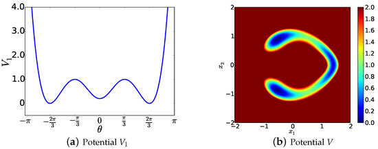
Figure 1. (a) Function $V_1$ as a function of angle θ; (b) Potential V defined in (74) with parameter $ϵ=0.05$.

The main purpose of this numerical experiment is to demonstrate that the leading eigenvalues of the operator $-\mathcal{L}$ corresponding to dynamics (73) can be approximated with the help of its effective dynamics, provided that the reaction coordinate function as well as the basis functions are chosen appropriately.

We choose parameters $\beta =4.0$ and $ϵ=0.05$ in the following numerical experiment. In fact, for this two-dimensional problem, it is possible to directly solve the eigenproblem (5) by discretizing the operator $\mathcal{L}$. First of all, we note that the generator can be written as $\mathcal{L}=\frac{e^{\beta V}}{\beta }\nabla (e^{-\beta V}\nabla )$. Defining the operator $\mathcal{D}$ such that $\mathcal{D}f=e^{-\frac{\beta }{2}V}f$ for a function f, it is straightforward to see that the operator $-{\mathcal{L}}_{\mathcal{D}}=-\mathcal{D}\mathcal{L}{\mathcal{D}}^{-1}$ has the same eigenvalues ${\lambda }_i$ as $-\mathcal{L}$ and the corresponding eigenfunctions are given by ${\phi }_i^{\mathcal{D}}=\mathcal{D}{\phi }_i=e^{-\frac{\beta }{2}V}{\phi }_i$, where ${\phi }_i$ are the eigenfunctions of $-\mathcal{L}$. Furthermore, ${\mathcal{L}}_{\mathcal{D}}$ is a self-adjoint operator under the standard $L^2$ inner product. Instead of $-\mathcal{L}$, we will work with $-{\mathcal{L}}_{\mathcal{D}}$ and solve the eigenproblem $-{\mathcal{L}}_{\mathcal{D}}f=\lambda f$ because the discretized matrix will be symmetric and the corresponding eigenfunctions ${\phi }_i^{\mathcal{D}}$ decay rapidly.

Taking into account the profile of the potential V in Figure 1b, we truncate the whole space ${\mathbb{R}}^2$ into a finite domain $[-2,2]\times [-2,2]$, which is then discretized using a $500\times 500$ uniform mesh, leading to the cell resolution $\mathrm{\Delta }{x}_1=\mathrm{\Delta }{x}_2=\frac{4}{500}=0.008$. For $1\le i,j\le 500$, let $f_{i,j},V_{i,j}$ denote the values of the functions f, V evaluated at state $\left(-2.0+(i-\frac{1}{2})\mathrm{\Delta }{x}_1,-2.0+(j-\frac{1}{2})\mathrm{\Delta }{x}_2\right)$, respectively. Other notations such as $V_{i\pm \frac{1}{2},j}$ are defined in a similar way. Approximating $-{\mathcal{L}}_{\mathcal{D}}f=-\frac{1}{\beta }{e}^{\frac{\beta }{2}V}\nabla \left(e^{-\beta V}\nabla (e^{\frac{\beta }{2}V}f)\right)$ by the centered finite difference scheme, we obtain,

$$\begin{array}{c}\hfill \begin{array}{cc}\hfill -{({\mathcal{L}}_{\mathcal{D}}f)}_{i,j}\approx & \frac{e^{\frac{\beta }{2}{V}_{i,j}}}{\beta }[\frac{e^{-\beta V_{i-\frac{1}{2},j}}}{\mathrm{\Delta }{x}_1}\frac{e^{\frac{\beta }{2}{V}_{i,j}}{f}_{i,j}-e^{\frac{\beta }{2}{V}_{i-1,j}}{f}_{i-1,j}}{\mathrm{\Delta }{x}_1}-\frac{e^{-\beta V_{i+\frac{1}{2},j}}}{\mathrm{\Delta }{x}_1}\frac{e^{\frac{\beta }{2}{V}_{i+1,j}}{f}_{i+1,j}-e^{\frac{\beta }{2}{V}_{i,j}}{f}_{i,j}}{\mathrm{\Delta }{x}_1}\hfill \\ & +\frac{e^{-\beta V_{i,j-\frac{1}{2}}}}{\mathrm{\Delta }{x}_2}\frac{e^{\frac{\beta }{2}{V}_{i,j}}{f}_{i,j}-e^{\frac{\beta }{2}{V}_{i,j-1}}{f}_{i,j-1}}{\mathrm{\Delta }{x}_2}-\frac{e^{-\beta V_{i,j+\frac{1}{2}}}}{\mathrm{\Delta }{x}_2}\frac{e^{\frac{\beta }{2}{V}_{i,j+1}}{f}_{i,j+1}-e^{\frac{\beta }{2}{V}_{i,j}}{f}_{i,j}}{\mathrm{\Delta }{x}_2}],\hfill \end{array}\end{array}$$

(76)

for $1<i,j<500$. For boundary cells, the Neumann condition is applied when the neighboring cells are lying outside of the truncated domain. From (76), it can be observed that the resulting discretization matrix is both symmetric and sparse. Solving the eigenvalues of this matrix (of order 250,000 ) using the Krylov–Schur method through the numerical package SLEPc [36], we obtain the first four eigenvalues,

$$\begin{array}{c}\hfill {\lambda }_0=0.000,{\lambda }_1=0.010,{\lambda }_2=0.044,{\lambda }_3=1.458,\end{array}$$

(77)

with relative residual errors smaller than $1.1\times {10}^{-6}$. The corresponding eigenvectors are shown in Figure 2.

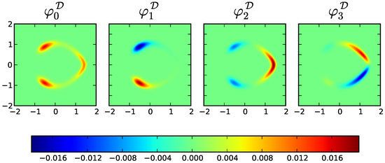
Figure 2. Eigenfunctions ${\phi }_i^{\mathcal{D}}$ of operator $-{\mathcal{L}}_{\mathcal{D}}$ corresponding to the first four eigenvalues in (77).

With the above reference result at hand, we continue to study the approximation quality of the effective dynamics with respect to the leading eigenvalues. For this purpose, we choose the reaction coordinate function as $\xi (x)=\theta (x)\in [-\pi ,\pi ]$, i.e., our reaction coordinate is the angle of the polar coordinate representation. Direct calculation shows that the coefficients $\tilde{b},\tilde{\sigma }$ in (32) reduces to,

$$\begin{array}{c}\hfill \begin{array}{c}\hfill \tilde{b}(z)=\mathbf{P}\left(-\nabla V·\nabla \theta \right)(z),\tilde{a}(z)=(\tilde{\sigma }{\tilde{\sigma }}^T)(z)=\mathbf{P}\left(\frac{1}{r^2}\right)(z),z\in [-\pi ,\pi ].\end{array}\end{array}$$

(78)

Discretizing the interval $[-\pi ,\pi ]$ into 1000 subintervals and applying the projection scheme proposed in [34] for each fixed $z=-\pi +\frac{2\pi j}{1000}$, $0\le j\le 1000$, we can compute the coefficients of the effective dynamics; the resulting profiles are shown in Figure 3a,b. After these preparations, we can generate trajectories of the effective dynamics by simulating the SDE (31) using standard time stepping schemes. As shown in Figure 3c, the effective dynamics spend long times around values $-\frac{2\pi }{3},0$ and $\frac{2\pi }{3}$, which is accordance with the behavior of dynamics (73) as well as with the profile of the potential V in Figure 1b. Since the effective dynamics is one-dimensional, we can also discretize its infinitesimal generator $\tilde{\mathcal{L}}$ in (33) and compute the eigenvalues of $-\tilde{\mathcal{L}}$ which gives,

$$\begin{array}{c}\hfill {\tilde{\lambda }}_0=0.000,{\tilde{\lambda }}_1=0.012,{\tilde{\lambda }}_2=0.044,{\tilde{\lambda }}_3=2.068.\end{array}$$

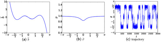
Figure 3. (a,b) Coefficients $\tilde{b}$ and $\tilde{\sigma }$ as given in (78). For each $z=-\pi +\frac{2\pi j}{1000}$, $0\le j\le 1000$, the coefficients $\tilde{b}(z)$, $\tilde{\sigma }(z)$ are estimated by generating a trajectory of the constrained version of dynamics (73) using the projection scheme proposed in [34] with the time step size $2\times {10}^{-5}$, and $3\times {10}^6$ steps are simulated; (c) A typical sample trajectory of the effective dynamics for dynamics (73) with reaction coordinate function $\xi (x)=\theta (x)$.

Comparing to (77), we conclude that the eigenvalues ${\lambda }_0,{\lambda }_1,{\lambda }_2$ of the original dynamics (73) are quite well approximated by those of the effective dynamics.

As the final step of our experiment, we test the trajectory-based method proposed in SubSection 5.1. First of all, we define basis functions ${\tilde{\psi }}_1(z)\equiv 1.0$ and ${\tilde{\psi }}_i(z)=\exp \left(-\frac{{(z-c_i)}^2}{2{\gamma }_i^2}\right)$, $2\le i\le 7$, where,

$$\begin{array}{c}\hfill c_i=\left\{-\frac{2\pi }{3},-\frac{2\pi }{3},0,0,\frac{2\pi }{3},\frac{2\pi }{3}\right\},r_i=\left\{0.4,0.7,0.4,0.7,0.4,0.7\right\}.\end{array}$$

That is, we have located two Gaussian-like basis functions with different radiuses ($0.4$ and $0.7$) at each of the three local minima $\theta =0,\pm \frac{2\pi }{3}$. The matrices S and C are then estimated according to (58) and (60) by generating four long trajectories of the effective dynamics with time step size $\mathrm{\Delta }t=5\times {10}^{-4}$, and parameters $\tau =20\mathrm{\Delta }t$, $M_0=1000$, $M=2\times {10}^7$ are used for each trajectories. Solving the generalized matrix eigenproblem $CX=\lambda SX$, we obtain the leading eigenvalues,

$$\begin{array}{c}\hfill {\tilde{\lambda }}_0=0.000,{\tilde{\lambda }}_1=0.013,{\tilde{\lambda }}_2=0.045,{\tilde{\lambda }}_3=3.776.\end{array}$$

As before, we conclude that the eigenvalues ${\lambda }_0$, ${\lambda }_1$, ${\lambda }_2$ of the original dynamics are relatively well approximated.

7. Conclusions

In this work we have studied the approximation of eigenvalues and eigenfunctions of the infinitesimal generator associated with the longest relaxation processes of diffusive processes in energy landscapes. Following the previous studies on transfer operators, we consider the Galerkin discretization method, the variational approach and the effective dynamics given by a low-dimensional reaction coordinate for solving the eigenvalue problem in application to the generator. It turns out that: (1) there are rather similar results for the approximation error of the three methods; and (2) the first two methods lead to the same generalized matrix eigenproblem while the third can be used for efficient estimation of the associated coefficient matrices.

Before we conclude, it is worth mentioning several issues which go beyond the scope of our current work. Firstly, while we have assumed that the dynamics are driven by the gradient of a potential function, we emphasize that the analysis in the current work can be directly applied to more general reversible processes (see [23] for details). Secondly, for non-reversible dynamics, as, for example, for Langevin dynamics, it is not immediately clear how the results in the current work can be applied. However, the approach in [9] (Section 5.3), shows that the extended reversibility of Langevin dynamics may well allow for a generalization of our results. Thirdly, for the numerical algorithms which are briefly outlined in Section 5, both the numerical analysis and their applications to more complicated systems need to be further investigated. Lastly, both the analysis and the algorithms in our current work depend on the choice of the reaction coordinate function. Different choices will have different approximation qualities of the eigenvalues/eigenfunctions of the system [21,23,37]. Algorithmic identification of reaction coordinate functions for high-dimensional systems is a challenging problem and has attracted considerable attention; most approaches utilize machine learning approaches [38], while the relation between identification and effective dynamics has only been explored recently [39]. All of these issues are topics of ongoing research.

References

- Schütte, C.; Fischer, A.; Huisinga, W.; Deuflhard, P. A direct approach to conformational dynamics based on hybrid Monte Carlo. J. Comput. Phys. 1999, 151, 146–168. [Google Scholar]
- Pande, V.S.; Beauchamp, K.; Bowman, G.R. Everything you wanted to know about Markov state models but were afraid to ask. Methods 2010, 52, 99–105. [Google Scholar]
- Pérez-Hernández, G.; Paul, F.; Giorgino, T.; De Fabritiis, G.; Noé, F. Identification of slow molecular order parameters for Markov model construction. J. Chem. Phys. 2013, 139, 015102. [Google Scholar]
- Nüske, F.; Schneider, R.; Vitalini, F.; Noé, F. Variational tensor approach for approximating the rare-event kinetics of macromolecular systems. J. Chem. Phys. 2016, 144, 054105. [Google Scholar]
- Noé, F.; Schütte, C.; Vanden-Eijnden, E.; Reich, L.; Weikl, T.R. Constructing the full ensemble of folding pathways from short off-equilibrium simulations. Proc. Natl. Acad. Sci. USA 2009, 106, 19011–19016. [Google Scholar]
- Bowman, G.R.; Pande, V.S.; Noé, F. (Eds.) Advances in Experimental Medicine and Biology. In An Introduction to Markov State Models and Their Application to Long Timescale Molecular Simulation; Springer: Dordrecht, The Netherlands, 2014; Volume 797. [Google Scholar]
- Noé, F.; Nüske, F. A variational approach to modeling slow processes in stochastic dynamical systems. Multiscale Model. Simul. 2013, 11, 635–655. [Google Scholar]
- Nüske, F.; Keller, B.G.; Pérez-Hernández, G.; Mey, A.; Noé, F. Variational approach to molecular kinetics. J. Chem. Theory Comput. 2014, 10, 1739–1752. [Google Scholar]
- Schütte, C.; Sarich, M. Metastability and Markov State Models in Molecular Dynamics: Modeling, Analysis, Algorithmic Approaches; Courant Lecture Notes; American Mathematical Society/Courant Institute of Mathematical Science: New York, NY, USA, 2014. [Google Scholar]
- Schütte, C.; Noé, F.; Lu, J.; Sarich, M.; Vanden-Eijnden, E. Markov state models based on milestoning. J. Chem. Phys. 2011, 134, 204105. [Google Scholar]
- Torrie, G.M.; Valleau, J.P. Nonphysical sampling distributions in Monte Carlo free-energy estimation: Umbrella sampling. J. Comput. Phys. 1977, 23, 187–199. [Google Scholar]
- Kumar, S.; Rosenberg, J.M.; Bouzida, D.; Swendsen, R.H.; Kollman, P.A. THE weighted histogram analysis method for free-energy calculations on biomolecules. I. The method. J. Comput. Chem. 1992, 13, 1011–1021. [Google Scholar]
- Laio, A.; Parrinello, M. Escaping free-energy minima. Proc. Natl. Acad. Sci. USA 2002, 99, 12562–12566. [Google Scholar]
- Laio, A.; Gervasio, F.L. Metadynamics: A method to simulate rare events and reconstruct the free energy in biophysics, chemistry and material science. Rep. Prog. Phys. 2008, 71, 126601. [Google Scholar]
- Ciccotti, G.; Kapral, R.; Vanden-Eijnden, E. Blue moon sampling, vectorial eeaction coordinates, and unbiased constrained dynamics. ChemPhysChem 2005, 6, 1809–1814. [Google Scholar]
- Darve, E.; Rodríguez-Gömez, D.; Pohorille, A. Adaptive biasing force method for scalar and vector free energy calculations. J. Chem. Phys. 2008, 128, 144120. [Google Scholar]
- Maragliano, L.; Vanden-Eijnden, E. A temperature accelerated method for sampling free energy and determining reaction pathways in rare events simulations. Chem. Phys. Lett. 2006, 426, 168–175. [Google Scholar]
- Faradjian, A.K.; Elber, R. Computing time scales from reaction coordinates by milestoning. J. Chem. Phys. 2004, 120, 10880–10889. [Google Scholar]
- Moroni, D.; van Erp, T.; Bolhuis, P. Investigating rare events by transition interface sampling. Physica A 2004, 340, 395–401. [Google Scholar]
- Becker, N.B.; Allen, R.J.; ten Wolde, P.R. Non-stationary forward flux sampling. J. Chem. Phys. 2012, 136, 174118. [Google Scholar]
- Legoll, F.; Lelièvre, T. Effective dynamics using conditional expectations. Nonlinearity 2010, 23, 2131–2163. [Google Scholar]
- Froyland, G.; Gottwald, G.A.; Hammerlindl, A. A computational method to extract macroscopic variables and their dynamics in multiscale systems. SIAM J. Appl. Dyn. Syst. 2014, 13, 1816–1846. [Google Scholar]
- Zhang, W.; Hartmann, C.; Schutte, C. Effective dynamics along given reaction coordinates, and reaction rate theory. Faraday Discuss. 2016, 195, 365–394. [Google Scholar]
- Kevrekidis, I.G.; Gear, C.W.; Hummer, G. Equation-free: The computer-aided analysis of complex multiscale systems. AIChE J. 2004, 50, 1346–1355. [Google Scholar]
- Kevrekidis, I.G.; Samaey, G. Equation-free multiscale computation: Algorithms and applications. Annu. Rev. Phys. Chem. 2009, 60, 321–344. [Google Scholar]
- Kevrekidis, I.G.; Gear, C.W.; Hyman, J.M.; Kevrekidid, P.G.; Runborg, O.; Theodoropoulos, C. Equation-free, coarse-grained multiscale computation: Enabling mocroscopic simulators to perform system-level analysis. Commun. Math. Sci. 2003, 1, 715–762. [Google Scholar]
- Prinz, J.H.; Wu, H.; Sarich, M.; Keller, B.; Senne, M.; Held, M.; Chodera, J.D.; Schütte, C.; Noé, F. Markov models of molecular kinetics: Generation and validation. J. Chem. Phys. 2011, 134, 174105. [Google Scholar]
- Djurdjevac, N.; Sarich, M.; Schütte, C. Estimating the eigenvalue error of Markov state models. Multiscale Model. Simul. 2012, 10, 61–81. [Google Scholar]
- Sarich, M.; Noé, F.; Schütte, C. On the approximation quality of Markov state models. Multiscale Model. Simul. 2010, 8, 1154–1177. [Google Scholar]
- Sarich, M.; Schütte, C. Approximating selected non-dominant timescales by Markov state models. Comm. Math. Sci. 2012, 10, 1001–1013. [Google Scholar]
- Mattingly, J.C.; Stuart, A.M.; Higham, D.J. Ergodicity for SDEs and approximations: locally Lipschitz vector fields and degenerate noise. Stoch. Proc. Appl. 2002, 101, 185–232. [Google Scholar]
- Schütte, C.; Huisinga, W.; Deuflhard, P. Transfer operator approach to conformational dynamics in biomolecular systems. In Ergodic Theory, Analysis, and Efficient Simulation of Dynamical Systems; Fiedler, B., Ed.; Springer: Berlin/Heidelberg, Germany, 2001; pp. 191–223. [Google Scholar]
- Gyöngy, I. Mimicking the one-dimensional marginal distributions of processes having an Ito differential. Probab. Theory Relat. Fields 1986, 71, 501–516. [Google Scholar]
- Ciccotti, G.; Lelièvre, T.; Vanden-Eijnden, E. Projection of diffusions on submanifolds: Application to mean force computation. Commun. Pure Appl. Math. 2008, 61, 371–408. [Google Scholar]
- Lelièvre, T.; Rousset, M.; Stoltz, G. Langevin dynamics with constraints and computation of free energy differences. Math. Comput. 2012, 81, 2071–2125. [Google Scholar]
- Hernandez, V.; Roman, J.E.; Vidal, V. SLEPc: A scalable and flexible toolkit for the solution of eigenvalue problems. ACM Trans. Math. Softw. 2005, 31, 351–362. [Google Scholar]
- Hartmann, C.; Schütte, C.; Zhang, W. Model reduction algorithms for optimal control and importance sampling of diffusions. Nonlinearity 2016, 29, 2298–2326. [Google Scholar]
- Rohrdanz, M.A.; Zheng, W.; Maggioni, M.; Clementi, C. Determination of reaction coordinates via locally scaled diffusion map. J. Chem. Phys. 2011, 134, 124116. [Google Scholar]
- Bittracher, A.; Koltai, P.; Klus, S.; Banisch, R.; Dellnitz, M.; Schütte, C. Transition manifolds of complex metastable systems: Theory and data-driven computation of effective dynamics. J. Nonlinear Sci. 2017, submitted. [Google Scholar]
© 2017 by the authors. Licensee MDPI, Basel, Switzerland. This article is an open access article distributed under the terms and conditions of the Creative Commons Attribution (CC BY) license (http://creativecommons.org/licenses/by/4.0/).