Matrix Information Geometry for Signal Detection via Hybrid MPI/OpenMP
Abstract
1. Introduction
2. The Matrix Information Geometric Signal Detection Method
2.1. Mapping from the Sample Data to an HPD Manifold
2.2. Derivation of the Riemannian Mean Matrix
2.3. Computational Complexity of the Algorithm
| Algorithm 1MIGSD (M, K, PFA, Pd_D) |
 |
3. High-Performance Computing-Based MIGSD Method
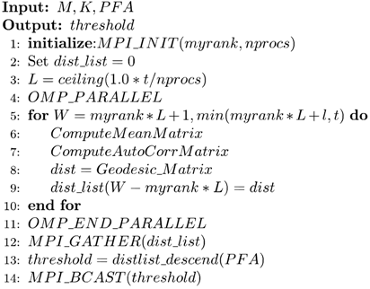
3.1. Our Efforts in the Training Step
| Algorithm 2 Training (M, K, PFA, threshold) |
 |
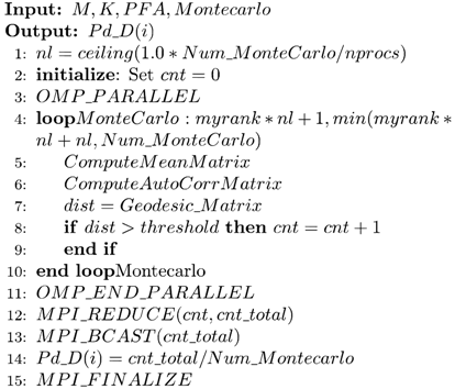
3.2. Our Efforts in the Working Step
| Algorithm 3 Working (M, K, threshold, Montecarlo) |
 |
4. Numerical Experiments
4.1. Time Cost in the Serial MIGSD Program
4.2. Parallel Performance in HPC-BASED MIGSD Program
4.3. Detection Performances for Various Dimensions of the Matrix
5. Discussion
Author Contributions
Funding
Conflicts of Interest
References
- Amrouche, N.; Khenchaf, A.; Berkani, D. Detection and tracking targets under low SNR. In Proceedings of the International Conference on Industrial Technology, Toronto, ON, Canada, 22–25 March 2017. [Google Scholar]
- Amrouche, N.; Khenchaf, A.; Berkani, D. Tracking and Detecting moving weak Targets. J. Adv. Sci. Technol. Eng. Syst. J. 2018, 3, 467–471. [Google Scholar] [CrossRef][Green Version]
- Amari, S. Information geometry of the EM and em algorithms for neural networks. Neural Netw. 1995, 8, 1379–1408. [Google Scholar] [CrossRef]
- Cao, W.; Liu, N.; Kong, Q.; Feng, H. Content-based image retrieval using high-dimensional information geometry. Sci. China Inf. Sci. 2014, 57, 1–11. [Google Scholar] [CrossRef]
- Mio, W.; Badlyans, D.; Liu, X. A computational approach to Fisher information geometry with applications to image analysis. In Proceedings of the International Workshop on Energy Minimization Methods in Computer Vision and Pattern Recognition, St. Augustine, FL, USA, 9–11 November 2005; pp. 18–33. [Google Scholar]
- Formont, P.; Ovarlez, J.P.; Pascal, F. On the use of matrix information geometry for polarimetric SAR image classification. In Matrix Information Geometry; Springer: Berlin/Heidelberg, Germany, 2013; pp. 257–276. [Google Scholar]
- Hua, X.; Shi, Y.; Zeng, Y.; Chen, C.; Lu, W.; Cheng, Y.; Wang, H. A divergence mean-based geometric detector with a pre-processing procedure. Measurement 2019, 131, 640–646. [Google Scholar] [CrossRef]
- Hua, X.; Cheng, Y.; Wang, H.; Qin, Y.; Chen, D. Geometric target detection based on total Bregman divergence. Digit. Signal Process. 2018, 75, 232–241. [Google Scholar] [CrossRef]
- Hua, X.; Cheng, Y.; Li, Y.; Shi, Y.; Wang, H.; Qin, Y. Information Geometry for Covariance Estimation in Heterogeneous Clutter with Total Bregman Divergence. Entropy 2018, 20, 258. [Google Scholar] [CrossRef]
- Hua, X.; Cheng, Y.; Wang, H.; Qin, Y.; Li, Y. Geometric means and medians with applications to target detection. IET Signal Process. 2017, 11, 711–720. [Google Scholar] [CrossRef]
- Hua, X.; Cheng, Y.; Li, Y.; Shi, Y.; Wang, H.; Qin, Y. Target detection in sea clutter via weighted averaging filter on the Riemannian manifold. Aerosp. Sci. Technol. 2017, 70, 47–54. [Google Scholar] [CrossRef]
- Hua, X.; Fan, H.; Cheng, Y.; Wang, H.; Qin, Y. Information Geometry for Radar Target Detection with Total Jensen–Bregman Divergence. Entropy 2018, 20, 256. [Google Scholar] [CrossRef]
- Cherian, A.; Sra, S. Riemannian dictionary learning and sparse coding for positive definite matrices. IEEE Trans. Neural Netw. Learn. Syst. 2016, 28, 2859–2871. [Google Scholar] [CrossRef]
- Amari, S.I.; Han, T. Statistical inference under multiterminal rate restrictions: A differential geometric approach. IEEE Trans. Inf. Theory 1989, 35, 217–227. [Google Scholar] [CrossRef]
- Kass, R.E.; Vos, P.W. Geometrical Foundations of Asymptotic Inference; John Wiley & Sons: Hoboken, NJ, USA, 2011; Volume 908. [Google Scholar]
- Amari, S.I. Information geometry on hierarchy of probability distributions. IEEE Trans. Inf. Theory 2001, 47, 1701–1711. [Google Scholar] [CrossRef]
- Barbaresco, F. New foundation of radar Doppler signal processing based on advanced differential geometry of symmetric spaces: Doppler matrix CFAR and radar application. In Proceedings of the International Radar Conference, Bordeaux, France, 12–16 October 2009. [Google Scholar]
- Lapuyade-Lahorgue, J.; Barbaresco, F. Radar detection using Siegel distance between autoregressive processes, application to HF and X-band radar. In Proceedings of the IEEE Radar Conference, Rome, Italy, 26–30 May 2008; pp. 1–6. [Google Scholar]
- Barbaresco, F. Robust statistical radar processing in Fréchet metric space: OS-HDR-CFAR and OS-STAP processing in Siegel homogeneous bounded domains. In Proceedings of the 12th International Radar Symposium (IRS), Leipzig, Germany, 7–9 September 2011; pp. 639–644. [Google Scholar]
- Hua, X.; Cheng, Y.; Wang, H.; Qin, Y.; Li, Y.; Zhang, W. Matrix CFAR detectors based on symmetrized Kullback–Leibler and total Kullback–Leibler divergences. Digit. Signal Process. 2017, 69, 106–116. [Google Scholar] [CrossRef]
- Hua, T.; Jianchun, B.; Hong, Y. Parallelization of the semi-Lagrangian shallow-water model using MPI techniques. Q. J. Appl. Meteorol. 2004, 4, 417–426. [Google Scholar]
- Jordi, A.; Wang, D.P. sbPOM: A parallel implementation of Princenton Ocean Model. Environ. Model. Softw. 2012, 38, 59–61. [Google Scholar] [CrossRef]
- Cowles, G.W. Parallelization of the FVCOM coastal ocean model. Int. J. High Perform. Comput. Appl. 2008, 22, 177–193. [Google Scholar] [CrossRef]
- Chandra, R.; Dagum, L.; Kohr, D.; Maydan, D.; McDonald, J.; Menon, R. Parallel Programming in OpenMP; Morgan Kaufmann: San Francisco, CA, USA, 2001. [Google Scholar]
- Breshears, C.P.; Luong, P. Comparison of openmp and pthreads within a coastal ocean circulation model code. In Proceedings of the Workshop on OpenMP Applications and Tools, San Diego, CA, USA, 13 July 2000. [Google Scholar]
- Malfetti, P. Application of OpenMP to weather, wave and ocean codes. Sci. Program. 2001, 9, 99–107. [Google Scholar] [CrossRef]
- Jang, H.; Park, A.; Jung, K. Neural network implementation using cuda and openmp. In Proceedings of the Digital Image Computing: Techniques and Applications, Canberra, Australia, 1–3 December 2008; pp. 155–161. [Google Scholar]
- Tarmyshov, K.B.; Müller-Plathe, F. Parallelizing a molecular dynamics algorithm on a multiprocessor workstation using OpenMP. J. Chem. Inf. Model. 2005, 45, 1943–1952. [Google Scholar] [CrossRef]
- Ayguade, E.; Gonzalez, M.; Martorell, X.; Jost, G. Employing nested OpenMP for the parallelization of multi-zone computational fluid dynamics applications. In Proceedings of the 18th International Parallel and Distributed Processing Symposium, Santa Fe, NM, USA, 26–30 April 2004; p. 6. [Google Scholar]
- Jacobsen, D.; Thibault, J.; Senocak, I. An MPI-CUDA implementation for massively parallel incompressible flow computations on multi-GPU clusters. In Proceedings of the 48th AIAA Aerospace Sciences Meeting Including the New Horizons Forum and Aerospace Exposition, Oriando, FL, USA, 4–7 January 2010. [Google Scholar]
- Namekata, D.; Iwasawa, M.; Nitadori, K.; Tanikawa, A.; Muranushi, T.; Wang, L.; Hosono, N.; Nomura, K.; Makino, J. Fortran interface layer of the framework for developing particle simulator FDPS. Publ. Astron. Soc. Jpn. 2018, 70, 70. [Google Scholar] [CrossRef]
- Gordon, A. A quick overview of OpenMP for multi-core programming. J. Comput. Sci. Coll. 2012, 28, 48. [Google Scholar]
- Mallón, D.A.; Taboada, G.L.; Teijeiro, C.; Tourino, J.; Fraguela, B.B.; Gómez, A.; Doallo, R.; Mourino, J.C. Performance evaluation of MPI, UPC and OpenMP on multicore architectures. In Proceedings of the·European Parallel Virtual Machine/Message Passing Interface Users’ Group Meeting, Espoo, Finland, 7–10 September 2009; pp. 174–184. [Google Scholar]
- Drosinos, N.; Koziris, N. Performance comparison of pure MPI vs hybrid MPI-OpenMP parallelization models on SMP clusters. In Proceedings of the 18th International Parallel and Distributed Processing Symposium, Santa Fe, NM, USA, 26–30 April 2004; p. 15. [Google Scholar]
- Chorley, M.J.; Walker, D.W. Performance analysis of a hybrid MPI/OpenMP application on multi-core clusters. J. Comput. Sci. 2010, 1, 168–174. [Google Scholar] [CrossRef]
- Rabenseifner, R.; Hager, G.; Jost, G. Hybrid MPI/OpenMP parallel programming on clusters of multi-core SMP nodes. In Proceedings of the 17th Euromicro international conference on parallel, distributed and network-based processing, Weimar, Germany, 18–20 February 2009; pp. 427–436. [Google Scholar]
- Rabenseifner, R.; Hager, G.; Jost, G.; Keller, R. Hybrid MPI and OpenMP parallel programming. In Proceedings of the PVM/MPI, Bonn, Germany, 17–20 September 2006; p. 11. [Google Scholar]
- Šipková, V.; Lúcny, A.; Gazák, M. Experiments with a Hybrid-Parallel Model of Weather Research and Forecasting (WRF) System. In Proceedings of the 6th International Workshop on Grid Computing for Complex Problems, Bratislava, Slovakia, 8–10 November 2010; p. 37. [Google Scholar]
- Geng, D.; Shen, W.; Cui, J.; Quan, L. The implementation of KMP algorithm based on MPI + OpenMP. In Proceedings of the 9th International Conference on Fuzzy Systems and Knowledge Discovery, Sichuan, China, 29–31 May 2012; pp. 2511–2514. [Google Scholar]
- Luong, P.; Breshears, C.P.; Ly, L.N. Application of multiblock grid and dual-level parallelism in coastal ocean circulation modeling. J. Sci. Comput. 2004, 20, 257–275. [Google Scholar] [CrossRef]
- Woodsend, K.; Gondzio, J. Hybrid MPI/OpenMP parallel linear support vector machine training. J. Mach. Learn. Res. 2009, 10, 1937–1953. [Google Scholar]
- Lee, D.; Vuduc, R.; Gray, A.G. A distributed kernel summation framework for general-dimension machine learning. In Proceedings of the SIAM International Conference on Data Mining, Anaheim, CA, USA, 26–28 April 2012; pp. 391–402. [Google Scholar]
- Mohanavalli, S.; Jaisakthi, S.; Aravindan, C. Strategies for parallelizing kmeans data clustering algorithm. In Proceedings of the International Conference on Advances in Information Technology and Mobile Communication, Anaheim, CA, USA, 3–7 December 2011; pp. 427–430. [Google Scholar]
- Götz, M.; Richerzhagen, M.; Bodenstein, C.; Cavallaro, G.; Glock, P.; Riedel, M.; Benediktsson, J.A. On scalable data mining techniques for earth science. Procedia Comput. Sci. 2015, 51, 2188–2197. [Google Scholar] [CrossRef]
- Peng, Y.; Wang, F. Cloud computing model based on MPI and OpenMP. In Proceedings of the 2nd International Conference on Computer Engineering and Technology, Chengdu, China, 16–18 April 2010. [Google Scholar]
- Arnaudon, M.; Barbaresco, F.; Yang, L. Medians and means in Riemannian geometry: Existence, uniqueness and computation. In Matrix Information Geometry; Springer: Berlin/Heidelberg, Germany, 2013; pp. 169–197. [Google Scholar]
- Bhatia, R.; Holbrook, J. Riemannian geometry and matrix geometric means. Linear Algebr. Appl. 2006, 413, 594–618. [Google Scholar] [CrossRef]


| Operation | Complexity |
|---|---|
| Vector addition | O(n) |
| Vector multiplication | O(n2) |
| Matrix addition | O(n2) |
| Matrix multiplication | O(n3) |
| Matrix eigenvalue | O(n3) |
| Matrix logarithm | O(n3) |
| Matrix inversion | O(n3) |
| Item | Values |
|---|---|
| 2 × CPU | Intel(R) Xeon(R) CPU E5-2692 v2 @ 2.20 GHz |
| Operating System | Kylin Linux |
| Kernel | 2.6.32-279-TH2 |
| MPI Version | MPICH Version 3.1.3 |
| GCC Version | GCC 4.4.7 |
| Compiler | Intel-compilers/15.0.1 |
| Experimental Groups | Elapsed Time (s) | Speed-Up |
|---|---|---|
| (a) 1 thread, 24 processes | 39.49 | 20.44 |
| (b) 2 thread, 12 processes | 41.61 | 19.40 |
| (c) 3 threads, 8 processes | 41.3 | 19.54 |
| (d) 4 threads, 6 processes | 41.50 | 19.54 |
| (e) 6 threads, 4 processes | 42.46 | 19.01 |
| (f) 8 threads, 3 processes | 42.53 | 19.00 |
| (g) 12 threads, 2 processes | 80.7 | 10.01 |
| (h) 24 threads, 1 process | 51.53 | 15.67 |
© 2019 by the authors. Licensee MDPI, Basel, Switzerland. This article is an open access article distributed under the terms and conditions of the Creative Commons Attribution (CC BY) license (http://creativecommons.org/licenses/by/4.0/).
Share and Cite
Feng, S.; Hua, X.; Wang, Y.; Lan, Q.; Zhu, X. Matrix Information Geometry for Signal Detection via Hybrid MPI/OpenMP. Entropy 2019, 21, 1184. https://doi.org/10.3390/e21121184
Feng S, Hua X, Wang Y, Lan Q, Zhu X. Matrix Information Geometry for Signal Detection via Hybrid MPI/OpenMP. Entropy. 2019; 21(12):1184. https://doi.org/10.3390/e21121184
Chicago/Turabian StyleFeng, Sheng, Xiaoqiang Hua, Yongxian Wang, Qiang Lan, and Xiaoqian Zhu. 2019. "Matrix Information Geometry for Signal Detection via Hybrid MPI/OpenMP" Entropy 21, no. 12: 1184. https://doi.org/10.3390/e21121184
APA StyleFeng, S., Hua, X., Wang, Y., Lan, Q., & Zhu, X. (2019). Matrix Information Geometry for Signal Detection via Hybrid MPI/OpenMP. Entropy, 21(12), 1184. https://doi.org/10.3390/e21121184


