Modulo Periodic Poisson Stable Solutions of Quasilinear Differential Equations

Abstract

In this paper, modulo periodic Poisson stable functions have been newly introduced. Quasilinear differential equations with modulo periodic Poisson stable coefficients are under investigation. The existence and uniqueness of asymptotically stable modulo periodic Poisson stable solutions have been proved. Numerical simulations, which illustrate the theoretical results are provided.

1. Introduction

The theory of differential equations is a doctrine on oscillations and recurrence, which are basic in science and technique. Oscillations are most preferable in engineering [1], while recurrence originates in celestial mechanics [2]. The ultimate recurrence is the Poisson stability [3,4,5]. Presently, needs for functions with irregular behavior are exceptionally strong in neuroscience and celestial dynamics, which is still in the developing mode. In the present research, we have decided to combine periodic dynamics with the phenomenon of Poisson stability. That is, one of simplest forms of oscillations is amalgamated with the most sophisticated type of recurrence. We hope that the choice can give a new push for the nonlinear analysis, which faces challenging problems of the real world and industry. The present product of the design are modulo periodic Poisson stable functions.

In paper [6], to strengthen the role of recurrence as a chaotic ingredient we have extended the Poisson stability to the unpredictability property. Thus, the Poincaré chaos has been determined, and one can say that the unpredictability implies chaos now. The unpredictable point of the Bebutov dynamics is the unpredictable function. In papers [7,8,9,10,11,12,13,14,15], we provided a dynamical method, how to construct Poisson stable functions. Deterministic and stochastic dynamics have been used. Deterministically unpredictable functions have been constructed as solutions of hybrid systems, consisting of discrete and differential equations [9,13,14], and randomly they are results of the Bernoulli process inserted into a linear differential equation [7,10,16]. Unpredictable oscillations in neural networks have been researched in [7,13,17,18,19].

In papers [8,9,10,14] and books [7,13], discussing existence of unpredictable solutions, we have developed a new method how to approve Poisson stable solutions, since unpredictable functions are a subset of Poisson stable functions, and to verify the unpredictability one must check, if the Poisson stability is valid. The method is distinctly different than the comparability method by character of recurrence, which was introduced in [20] and later has been realized in several articles [21,22,23,24,25,26,27]. Unlike papers [7,8,9,10,13,14,15,16,17,18,19], the present research is busy with the new type of Poisson stable functions. Correspondingly, it is the first time in literature, when quasilinear equations with Poisson stable coefficients are under investigation. Finally, the systems are approved with modulo periodic Poisson stable solutions. The newly invented method of verification of the Poisson stability joined with the presence of the periodic components in the recurrence has made possible the extension for the class of studied differential equations. In papers [21,22,23,24], quasilinear systems are with constant matrices of coefficients, and in our case, we research systems with periodic and, even with Poisson stable coefficients. Another significant novelty is the numerical simulation of the Poisson stable functions and solutions [7,9,13,14]. We believe that altogether, the present suggestions can shape a new interesting science direction, not only in the theoretical study of differential equations, but also they provide rich opportunities for applications in mechanics, electronics, artificial neural networks, neuroscience.

2. Preliminaries

Throughout the paper, $\mathbb{R}$ and $\mathbb{N}$ will stand for the set of real and natural numbers, respectively. Additionally, the norm ${\parallel u\parallel }_1={sup}_{t\in \mathbb{R}}\parallel u\left(t\right)\parallel ,$ where ${\displaystyle ∥u∥=\underset{1\le i\le n}{max}\left|u_i\right|,}$ $u=(u_1,\dots ,u_n),u_i\in \mathbb{R},i=1,2,...,n,$ will be used. Correspondingly, for a square matrix $A=\left\{a_{ij}\right\},i,j=1,2,...,n,$ the norm ${\displaystyle \parallel A\parallel =\underset{i=1,\dots ,n}{max}\sum _{j=1}^n\left|a_{ij}\right|}$ will be used.

Definition 1

([5]). A continuous and bounded function $\psi \left(t\right):\mathbb{R}\to {\mathbb{R}}^n$ is called Poisson stable, if there exists a sequence $t_k,$ which diverges to infinity such that the sequence $\psi (t+t_k)$ converges to $\psi \left(t\right)$ uniformly on bounded intervals of $\mathbb{R}.$

The sequence $t_k$ in the last definition is said to be Poisson sequence of the function $\psi \left(t\right).$

By Lemma A1 in the Appendix A, for a positive fixed $\omega$ there exist a subsequence $t_{k_l}$ of the Poisson sequence $t_k$ and a number ${\tau }_{\omega }$ such that $t_{k_l}\to {\tau }_{\omega }\left(mod\omega \right)$ as $l\to \infty .$ We shall call the number ${\tau }_{\omega }$ as the Poisson shift for the Poisson sequence $t_k$ with respect to the $\omega .$ It is not difficult to find that for the fixed $\omega$ the set of all Poisson shifts, $T_{\omega },$ is not empty, and it can consist of several and even infinite number elements. The number ${\kappa }_{\omega }=inf{T}_{\omega },$ $0\le {\kappa }_{\omega }<\omega ,$ is said to be the Poisson number for the Poisson sequence $t_k$ with respect to the number $\omega .$

Definition 2.

The sum $\varphi \left(t\right)+\psi \left(t\right)$ is said to be a modulo periodic Poisson stable ($MPPS$) function, if $\varphi \left(t\right)$ is a continuous periodic and $\psi \left(t\right)$ is a Poisson stable functions.

We shall call the function $\varphi \left(t\right)$ the periodic component and the function $\psi \left(t\right)$ the Poisson component of the $MPPS$ function in what follows.

Remark 1.

Duo to Lemma A3, an $MPPS$ function is a Poisson stable if ${\kappa }_{\omega }$ equals zero. Otherwise, without loss of generality, the sequence $\varphi (t+t_k)+\psi (t+t_k)$ converges on all compact subsets of the real axis to the function $\varphi (t+{\tau }_{\omega })+\psi \left(t\right),$ where ${\tau }_{\omega }$ is a nonzero Poisson shift for the sequence $t_k.$ Since of the periodicity of the function $\varphi \left(t\right),$ one can accept the last convergence as a special form of recurrence. In the next section, we shall consider it as a result of Theorem 1.

3. Main Results

3.1. Linear System of Differential Equations

Consider the following system

$$\begin{array}{c}\hfill x^{\prime }\left(t\right)=A\left(t\right)x\left(t\right)+\varphi \left(t\right)+\psi \left(t\right),\end{array}$$

(1)

where $t\in \mathbb{R},$ $x\in {\mathbb{R}}^n,$ $n\in \mathbb{N},$ $\varphi \left(t\right):\mathbb{R}\to {\mathbb{R}}^n$ and $\psi \left(t\right):\mathbb{R}\to {\mathbb{R}}^n$ are continuous functions, $A\left(t\right)$ is a continuous $n\times n$ matrix.

We assume that the following conditions are satisfied.

(C1) 

$A\left(t\right)$ is an $\omega -$ periodic matrix for a fixed positive $\omega ;$

(C2) 

$\varphi \left(t\right)$ is an $\omega -$ periodic function, and $\psi \left(t\right)$ is a Poisson stable function with a Poisson sequence $t_k;$

(C3) 

the Poisson number ${\kappa }_{\omega }$ for the sequence $t_k$ is equal to zero.

According to Definition 2 and condition (C2), the sum $\varphi \left(t\right)+\psi \left(t\right)$ is an $MPPS$ function, i.e., the linear system (1) is with $MPPS$ perturbation.

Let us consider the homogeneous system, associated with (1),

$$\begin{array}{c}\hfill x^{\prime }\left(t\right)=A\left(t\right)x\left(t\right).\end{array}$$

(2)

Let $X\left(t\right)$, $t\in \mathbb{R},$ is the fundamental matrix of the system (2) such that $X\left(0\right)=I,$ and I is the $n\times n$ identical matrix. Moreover, $X(t,s)$ is transition matrix of the system (2), which equal to $X\left(t\right)X^{-1}\left(s\right),$ and $X(t+\omega ,s+\omega )=X(t,s)$ for all $t,s\in \mathbb{R}.$

We assume that the following additional assumption is valid.

(C4) 

The multipliers of the system (2) in modulus are less than one.

It follows from the last condition that there exist positive numbers $K\ge 1$ and $\alpha$ such that

$$\begin{array}{c}\hfill \parallel X(t,s)\parallel \le K{e}^{-\alpha (t-s)},\end{array}$$

(3)

for $t\ge s$ [28].

Lemma 1.

If the inequality (3) is satisfied, then the following estimation is correct

$$\begin{array}{ccc}\hfill & & {\displaystyle \parallel X(t+\tau ,s+\tau )-X(t,s)\parallel \le \underset{t\in \mathbb{R}}{max}\parallel A(t+\tau )-A\left(t\right)\parallel \frac{2K^2}{{\alpha }^{2}e}{e}^{-\frac{\alpha }{2}(t-s)},}\hfill \end{array}$$

(4)

for $t\ge s$ and arbitrary real number $\tau .$

Proof. 

Since

$$\begin{array}{ccc}& & {\displaystyle \frac{dX(t+\tau ,s+\tau )}{dt}=A\left(t\right)X(t+\tau ,s+\tau )+(A(t+\tau )-A\left(t\right))X(t+\tau ,s+\tau ),}\hfill \end{array}$$

we have that

$$\begin{array}{ccc}& & {\displaystyle X(t+\tau ,s+\tau )=X(t,s)+{\int }_s^{t}X(t,u)(A(u+\tau )-A\left(u\right))X(u+\tau ,s+\tau )du.}\hfill \end{array}$$

That is why,

$$\begin{array}{ccc}& & {\displaystyle \parallel X(t+\tau ,s+\tau )-X(t,s)\parallel \le }\hfill \\ & & {\displaystyle {\int }_s^t\parallel X(t,u)\parallel \parallel A(u+\tau )-A\left(u\right)\parallel \parallel X(u+\tau ,s+\tau )\parallel du\le }\hfill \\ & & {\displaystyle \underset{t\in \mathbb{R}}{max}\parallel A(t+\tau )-A\left(t\right)\parallel {\int }_s^t{K}^2{e}^{-\alpha (t-s)}du=}\hfill \\ & & {\displaystyle \underset{t\in \mathbb{R}}{max}\parallel A(t+\tau )-A\left(t\right)\parallel \frac{K^2}{\alpha }{e}^{-\alpha (t-s)}(t-s)=}\hfill \\ & & {\displaystyle \underset{t\in \mathbb{R}}{max}\parallel A(t+\tau )-A\left(t\right)\parallel \frac{K^2}{\alpha }{e}^{-\frac{\alpha }{2}(t-s)}{e}^{-\frac{\alpha }{2}(t-s)}(t-s).}\hfill \end{array}$$

Since ${\displaystyle \underset{u\ge 0}{sup}{e}^{-\frac{\alpha }{2}u}u=\frac{2}{\alpha e},}$ the lemma is proved.  □

Theorem 1.

Assume that conditions (C1), (C2) and (C4) are valid. Then the system (1) admits a unique asymptotically stable $MPPS$ solution.

Proof. 

The bounded solution of system (1) has the form [28]

$$\begin{array}{ccc}\hfill & & x\left(t\right)={\int }_{-\infty }^{t}X(t,s)[\varphi \left(s\right)+\psi \left(s\right)]ds,t\in \mathbb{R}.\hfill \end{array}$$

(5)

One can write that $x\left(t\right)=x_{\varphi }\left(t\right)+x_{\psi }\left(t\right),$ where ${\displaystyle x_{\varphi }\left(t\right)={\int }_{-\infty }^{t}X(t,s)\varphi \left(s\right)ds}$ and ${\displaystyle x_{\psi }\left(t\right)={\int }_{-\infty }^{t}X(t,s)\psi \left(s\right)ds.}$

It is not difficult to show that the function $x_{\varphi }\left(t\right)$ is $\omega -$ periodic [29].

Next, we prove that the function $x_{\psi }\left(t\right)$ is Poisson stable. Fix arbitrary positive number $ϵ$ and interval $[a,b],$ $-\infty <a<b<\infty .$ We will show that for a large k it is true that $\parallel x_{\psi }(t+t_k)-x_{\psi }\left(t\right)\parallel <ϵ$ on $[a,b].$ Let us choose two numbers c and $\xi$ such that $c<a$ and $\xi$ is positive, satisfying the following inequalities,

$$\begin{array}{ccc}\hfill & & {\displaystyle \frac{4K^2{m}_{\psi }}{{\alpha }^{3}e}\xi <\frac{ϵ}{3},}\hfill \end{array}$$

(6)

$$\begin{array}{ccc}\hfill & & {\displaystyle \frac{2K{m}_{\psi }}{\alpha }{e}^{-\alpha (a-c)}<\frac{ϵ}{3},}\hfill \end{array}$$

(7)

and

$$\begin{array}{ccc}\hfill & & {\displaystyle \frac{K\xi }{\alpha }[1-e^{-\alpha (b-c)}]<\frac{ϵ}{3},}\hfill \end{array}$$

(8)

with ${\displaystyle m_{\psi }=\underset{t\in \mathbb{R}}{sup}\parallel \psi \left(t\right)\parallel .}$ By applying condition (C4), without loss of generality, for sufficiently large k we obtain that $\parallel A(t+t_k)-A\left(t\right)\parallel <\xi$ for all $t\in \mathbb{R},$ and $\parallel \psi (t+t_k)-\psi \left(t\right)\parallel <\xi$ for $t\in [c,b].$ Using Lemma 1 we attain that

$$\begin{array}{ccc}\hfill & & \parallel x_{\psi }(t+t_k)-x_{\psi }\left(t\right)\parallel = \parallel {\int }_{-\infty }^t\left(X(t+t_k,s+t_k)\psi (s+t_k)-X(t,s)\psi \left(s\right)\right)ds\parallel \le \hfill \\ & & {\int }_{-\infty }^t\parallel X(t+t_k,s+t_k)-X(t,s)\parallel \parallel \psi (s+t_k)\parallel ds +\hfill \\ & & {\int }_{-\infty }^t\parallel X(t,s)\parallel \parallel \psi (s+t_k)-\psi \left(s\right)\parallel ds=\hfill \\ & & {\int }_{-\infty }^t\parallel X(t+t_k,s+t_k)-X(t,s)\parallel \parallel \psi (s+t_k)\parallel ds +\hfill \\ & & {\int }_{-\infty }^c\parallel X(t,s)\parallel \parallel \psi (s+t_k)-\psi \left(s\right)\parallel ds +{\int }_c^t\parallel X(t,s)\parallel \parallel \psi (s+t_k)-\psi \left(s\right)\parallel ds\le \hfill \\ & & {\int }_{-\infty }^t\frac{2K^2\xi }{{\alpha }^{2}e}{e}^{-\frac{\alpha }{2}(t-s)}{m}_{\psi }ds+{\int }_{-\infty }^{t}2K{e}^{-\alpha (t-s)}{m}_{\psi }ds+{\int }_{-\infty }^{t}K{e}^{-\alpha (t-s)}\xi ds\le \hfill \\ & & \frac{4K^2\xi }{{\alpha }^{3}e}{m}_{\psi }+\frac{2K{m}_{\psi }}{\alpha }{e}^{-\alpha (a-c)}+\frac{K\xi }{\alpha }[1-e^{-\alpha (b-c)}].\hfill \end{array}$$

Now, the inequalities (6) to (8) imply that $\parallel x_{\psi }(t+t_k)-x_{\psi }\left(t\right)\parallel <ϵ,$ for $t\in [a,b].$ Therefore, the sequence $x_{\psi }(t+t_k)$ uniformly converges to $x_{\psi }\left(t\right)$ on each bounded interval. Thus, according to the Definition 2 the solution $x\left(t\right)$ of the system (1) is $MPPS$ function with the periodic component $x_{\varphi }\left(t\right)$ and the Poisson component $x_{\psi }\left(t\right).$ The asymptotic stability of the $MPPS$ solution can be verified in the same way as for the bounded solution of a linear inhomogeneous system [29].  □

The following examples show the validity of the obtained theoretical result.

Example 1.

Let us consider the following linear inhomogeneous system,

$$\begin{array}{c}\hfill \begin{array}{c}{x}_1^{\prime }=(-1+0.5sin\left(2t\right))x_1+2.5cos\left(t\right)+5.5{\Theta }^2\left(t\right),\hfill \\ x_2^{\prime }=(-2+0.25cos\left(t\right))x_2+2sin\left(2t\right)+1.7\Theta \left(t\right),\hfill \end{array}\end{array}$$

(9)

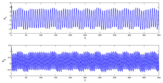
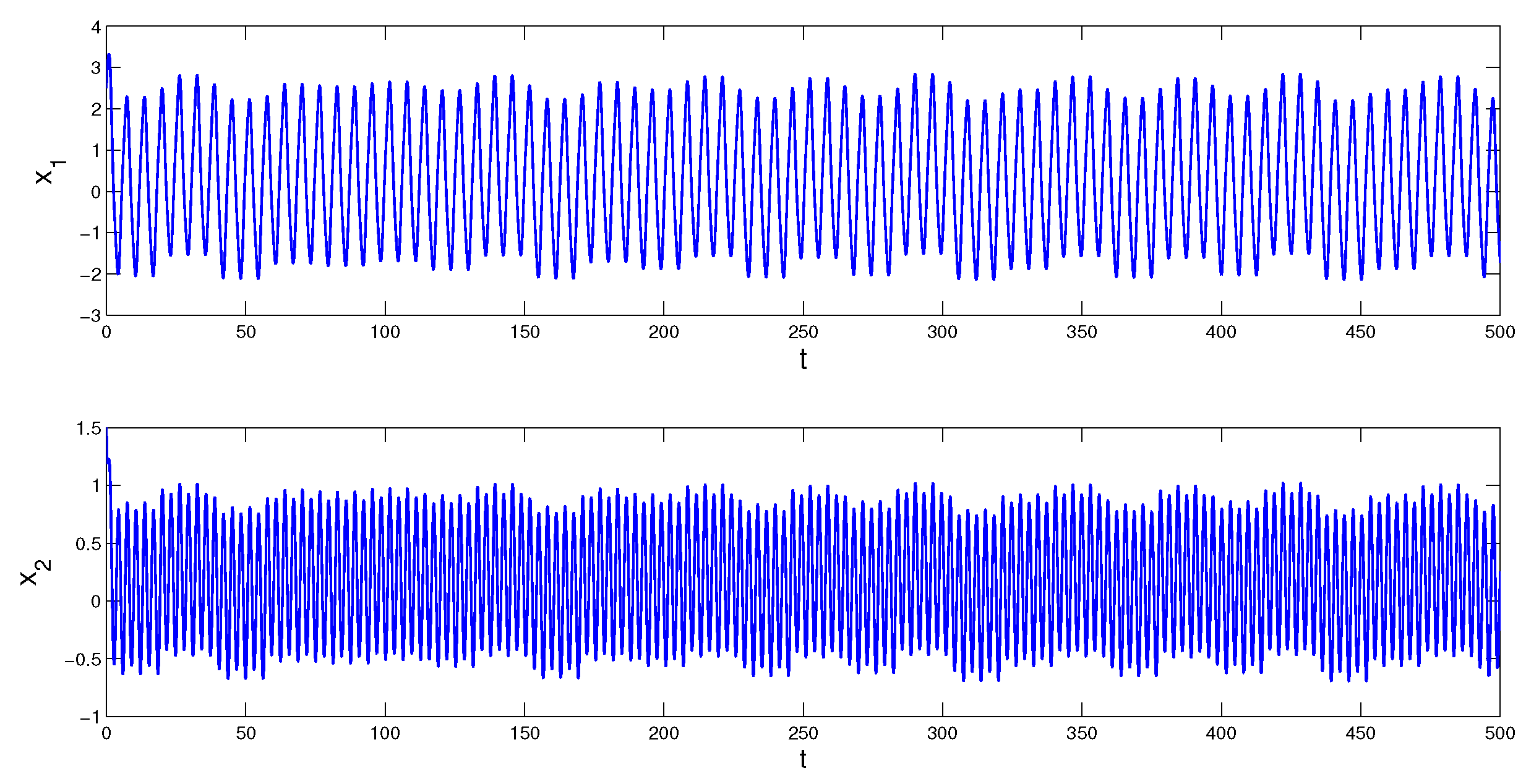
where $\Theta \left(t\right)={\int }_{-\infty }^t{e}^{-3(t-s)}{\Omega }_{(3.85;6\pi )}\left(s\right)ds$ is the Poisson stable function described in Appendix B. The perturbation is an $MPPS$ function with the periodic component $\varphi \left(t\right)={\left(2.5cos\left(t\right),2sin\left(2t\right)\right)}^T$ and the Poisson component $\psi \left(t\right)={\left(5.5{\Theta }^2\left(t\right),1.7\Theta \left(t\right)\right)}^T.$ The common period of the coefficient $A\left(t\right)$ and the periodic component $\varphi \left(t\right)$ is $2\pi .$ Since the function ${\Omega }_{(3.85,6\pi )}\left(t\right)$ is constructed on the intervals $[6\pi i,6\pi (i+1\left)\right),$ $i\in \mathbb{Z},$ for the Poisson sequence $t_k$ of the function $\Theta \left(t\right)$ there exists a subsequence $t_{k_l}$ such that $t_{k_l}\to 0\left(mod2\pi \right).$ Therefore, the Poisson number ${\kappa }_{\omega }=0.$ Condition (C4) is valid with the multipliers ${\rho }_1=e^{-2\pi },$ and ${\rho }_2=e^{-4\pi }.$ According to Theorem 1, the system admits a unique asymptotically stable $MPPS$ solution, $z\left(t\right).$ Since it is impossible to determine the initial value of the solution, we simulate a solution, which asymptotically approaches $z\left(t\right)$ as time increases. We depict in Figure 1 the coordinates of the solution $x\left(t\right),$ with initial values $x_1\left(0\right)=2.5$ and $x_2\left(0\right)=1.5,$ which visualizes the MPPS solution approximately. In Figure 2 the trajectory of the solution $x\left(t\right)$ is shown.

Figure 1. Coordinates of the solution $x\left(t\right)$ of system (9) with initial values $x_1\left(0\right)=2.5$ and $x_2\left(0\right)=1.5,$ which asymptotically converge to the coordinates of the $MPPS$ solution $z\left(t\right)$ of the system.

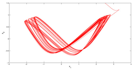
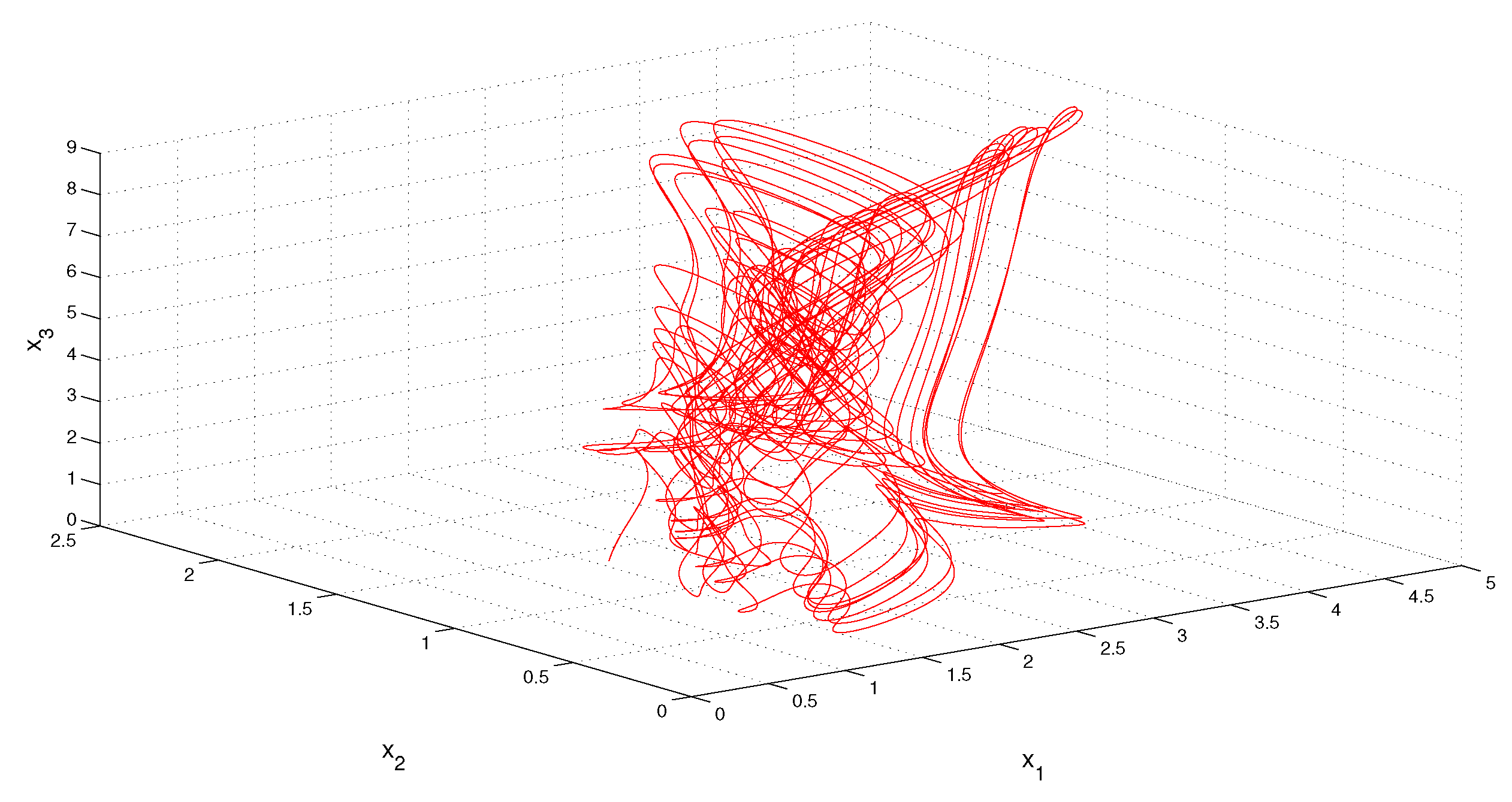
Figure 2. The trajectory of the solution $x\left(t\right)$ of the Equation (9), which asymptotically approaches the MPPS solution $z\left(t\right)$ of the system.

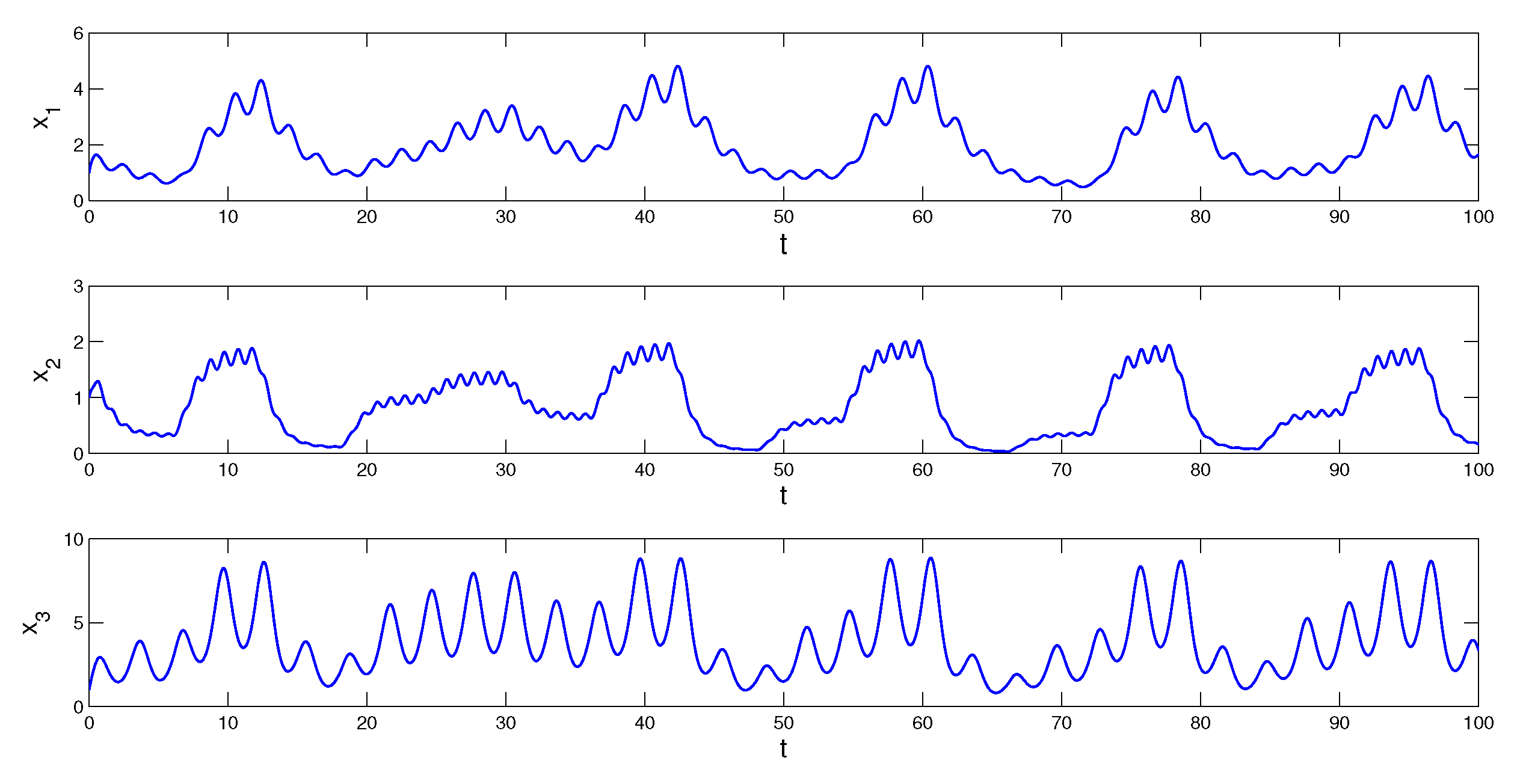
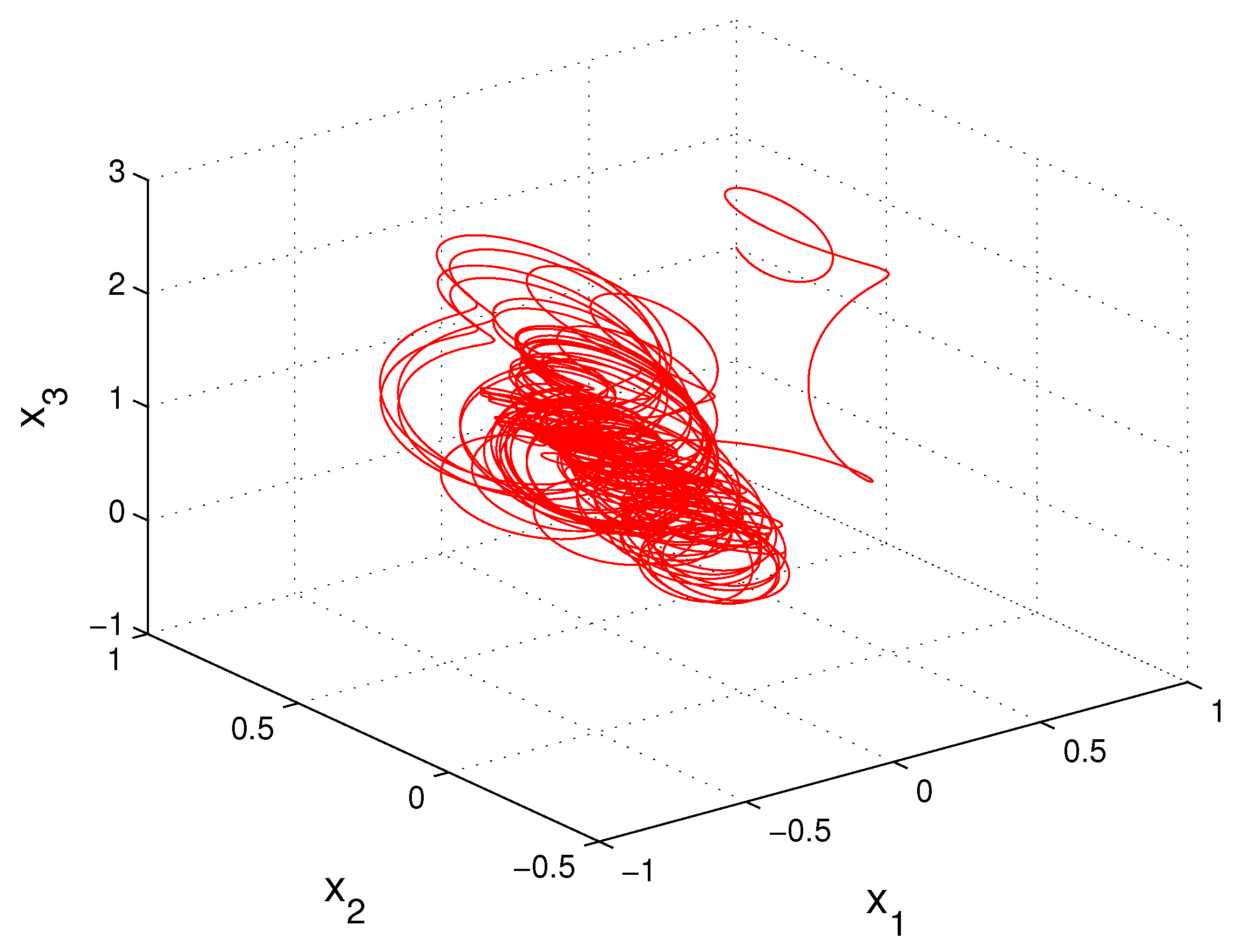
In the next example, the periodic component $\varphi \left(t\right)$ of the MPPS perturbation is absent, but the condition $\left(C2\right)$ is correct, since a constant function is of arbitrary period. It is remarkable to say that the absence of a proper non-constant periodic component makes the dynamics more irregular, this is seen in Figure 3 and Figure 4.

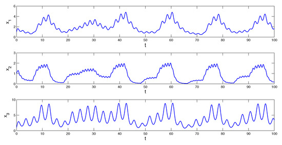
Figure 3. Coordinates of the solution $x\left(t\right),$ with initial values $x_1\left(0\right)=1,$ $x_2\left(0\right)=1$ and $x_3\left(0\right)=1,$ which asymptotically converge to the coordinates of the $MPPS$ solution of system (10).

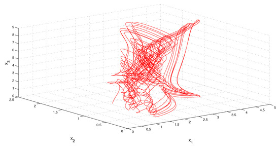
Figure 4. The trajectory of the solution, $x\left(t\right),$ of Equation (10), which asymptotically approaches the MPPS solution of the equation.

Example 2.

Consider the inhomogeneous linear system

$$\begin{array}{c}\hfill \begin{array}{c}{x}_1^{\prime }=(-0.25+0.5cos\left(\pi t\right))x_1+12{\Theta }^3\left(t\right),\hfill \\ x_2^{\prime }=(-1.5+si{n}^2\left(\pi t\right))x_2+8{\Theta }^2\left(t\right),\hfill \\ x_3^{\prime }=(-0.5+cos\left(\frac{2\pi }{3}t\right))x_3+6\Theta \left(t\right),\hfill \end{array}\end{array}$$

(10)

where $\Theta \left(t\right)={\int }_{-\infty }^t{e}^{-2(t-s)}{\Omega }_{(3.9;6)}\left(s\right)ds.$ The conditions (C1)–(C3) are satisfied, and condition (C4) is valid with multipliers ${\rho }_1=e^{-0.75},$ ${\rho }_2=e^{-3}$ and ${\rho }_3=e^{-1.5}.$ Consequently, there exists the unique asymptotically stable MPPS solution of the system (10). Figure 3 presents the coordinates of the solution $x\left(t\right)$ with initial values $x_1\left(0\right)=1,$ $x_2\left(0\right)=1$ and $x_3\left(0\right)=1.$ The coordinates of solution $x\left(t\right)$ approximate the coordinates of the $MPPS$ solution. The trajectory of the solution $x\left(t\right)$ is shown in Figure 4.

3.2. Quasilinear Differential Equations

The main object of the present section is the system of quasilinear differential equations

$$\begin{array}{c}\hfill x^{\prime }\left(t\right)=A\left(t\right)x+g(t,x)+\varphi \left(t\right)+\psi \left(t\right),\end{array}$$

(11)

where $t\in \mathbb{R},x\in {\mathbb{R}}^n,$n is a fixed natural number; $A\left(t\right)$ is $n-$ dimensional square matrix and satisfies to the condition (C1) and inequality (3); $g:\mathbb{R}\times U\to {\mathbb{R}}^n,g=(g_1,\dots ,g_n),$ $U=\{x\in {\mathbb{R}}^n,\parallel x\parallel <H\},$ where H is a fixed positive number; the functions $\varphi \left(t\right)$ and $\psi \left(t\right)$ satisfy conditions (C2) and (C3).

The following conditions on system (11) are required.

(C5) 

the function $g(t,x)$ is continuous and $\omega -$ periodic in $t;$

(C6) 

there exists a positive constant L such that $∥g(t,x_1)-g(t,x_2)∥\le L∥x_1-x_2∥$ for all $t\in \mathbb{R},x_1,x_2\in U.$

We denote ${\displaystyle \underset{\mathbb{R}\times U}{sup}\parallel g(t,x)\parallel =m_g,}$ ${\displaystyle \underset{t\in \mathbb{R}}{max}\parallel \varphi \left(t\right)\parallel =m_{\varphi }}$ and ${\displaystyle \underset{t\in \mathbb{R}}{sup}\parallel \psi \left(t\right)\parallel =m_{\psi }.}$

The following additional conditions will be needed:

(C7) 

${\displaystyle \frac{K(m_g+m_{\varphi }+m_{\psi })}{H}<\alpha ;}$

(C8) 

$KL<\alpha .$

For simplicity, we use the notation $F(t,x)=g(t,x)+\varphi \left(t\right)+\psi \left(t\right)$ in what follows.

According to [28], a bounded on the real axis function $y\left(t\right)$ is a solution of (11), if and only if it satisfies the equation

$$\begin{array}{ccc}\hfill & & y\left(t\right)={\int }_{-\infty }^{t}X(t,s)F(s,y\left(s\right))ds,t\in \mathbb{R}.\hfill \end{array}$$

(12)

Theorem 2.

If conditions (C1)–(C8) are valid, then the system (11) possesses a unique asymptotically stable Poisson stable solution.

Proof. 

Let $t_k$ is the Poisson sequence of the function $\psi \left(t\right)$ in the system (11). We denote by B the set of all Poisson stable functions $\nu \left(t\right)=({\nu }_1,{\nu }_2,...,{\nu }_n),$ ${\nu }_i\in \mathbb{R},$ $i=1,2,...,n,$ with common Poisson sequence $t_k,$ which satisfy ${∥\nu ∥}_1<H.$

Let us show that the B is a complete space. Consider a Cauchy sequence ${\theta }_m\left(t\right)$ in B, which converges to a limit function $\theta \left(t\right)$ on $\mathbb{R}$. We have that

$$\begin{array}{ccc}\hfill & & \parallel \theta (t+t_k)-\theta \left(t\right)\parallel <\parallel \theta (t+t_k)-{\theta }_m(t+t_k)\parallel +\parallel {\theta }_m(t+t_k)-{\theta }_m\left(t\right)\parallel +\hfill \\ & & \parallel {\theta }_m\left(t\right)-\theta \left(t\right)\parallel .\hfill \end{array}$$

(13)

for a fixed closed and bounded interval $I\subset \mathbb{R}.$ Now, one can take sufficiently large m and k such that each term on the right hand-side of (13) is smaller than $\frac{ϵ}{3}$ for a fixed positive $ϵ$ and $t\in I$, i.e., the sequence $\theta (t+t_k)$ uniformly converges to $\theta \left(t\right)$ on $I.$ Likewise, one can check that the limit function is uniformly continuous [28]. The completeness of B is shown.

Define the operator $\Pi$ on B such that

$$\begin{array}{ccc}\hfill & & \Pi \nu \left(t\right)={\int }_{-\infty }^{t}X(t,s)F(s,\nu \left(s\right))ds,t\in \mathbb{R}.\hfill \end{array}$$

(14)

Fix a function $\nu \left(t\right)$ that belongs to B. We have that

$$\begin{array}{ccc}& & {\displaystyle \parallel \Pi \nu \left(t\right)\parallel \le {\int }_{-\infty }^t\parallel X(t,s)\parallel \parallel F(s,\nu \left(s\right))\parallel ds\le \frac{K(m_g+m_{\varphi }+m_{\psi })}{\alpha }}\hfill \end{array}$$

for all $t\in \mathbb{R}.$ Therefore, by the condition (C7) it is true that ${∥\Pi \nu ∥}_1<H$.

Fix a positive number $ϵ$ and an interval $[a,b],$ $-\infty <a<b<\infty .$ Let us choose two numbers $c<a,$ and $\xi >0$ satisfying the inequalities

$$\begin{array}{c}\hfill \frac{4K^2\xi }{{\alpha }^{3}e}(m_g+m_{\varphi }+m_{\psi })<\frac{ϵ}{3},\end{array}$$

(15)

$$\begin{array}{c}\hfill {\displaystyle \frac{2K}{\alpha }(m_g+m_{\varphi }+m_{\psi })e^{-\alpha (a-c)}<\frac{ϵ}{3},}\end{array}$$

(16)

and

$$\begin{array}{c}\hfill {\displaystyle \frac{K\xi }{\alpha }[1-e^{-\alpha (b-c)}]<\frac{ϵ}{3}.}\end{array}$$

(17)

Using the condition (C4) and Lemmas A3 and A5 from Appendix A, without loss of generality, we obtain that $\parallel A(t+t_k)-A\left(t\right)\parallel <\xi$ for all $t\in \mathbb{R},$ and $\parallel F(t+t_k,\nu (t+t_k))-F(t,\nu \left(t\right))\parallel <\xi$ for $t\in [c,b]$ and sufficiently large $k.$ Then, applying the inequality (4), we obtain:

$$\begin{array}{ccc}\hfill & & \parallel \Pi \nu (t+t_k)-\Pi \nu \left(t\right)\parallel =\hfill \\ & & \parallel {\int }_{-\infty }^{t}X(t+t_k,s+t_k)F(s+t_k,\nu (s+t_k))ds-{\int }_{-\infty }^{t}X(t,s)F(s,\nu \left(s\right))ds\parallel \le \hfill \\ & & {\int }_{-\infty }^t\parallel X(t+t_k,s+t_k)-X(t,s)\parallel \parallel F(s+t_k,\nu (s+t_k))\parallel ds+\hfill \\ & & {\int }_{-\infty }^c\parallel X(t,s)\parallel \parallel F(s+t_k,\nu (s+t_k))-F(t,s)\parallel ds+\hfill \\ & & {\int }_c^t\parallel X(t,s)\parallel \parallel F(s+t_k,\nu (s+t_k))-F(t,s)\parallel ds\le \hfill \\ & & {\int }_{-\infty }^t\frac{2K^2\xi }{{\alpha }^{2}e}{e}^{-\frac{\alpha }{2}(t-s)}(m_g+m_{\varphi }+m_{\psi })ds+\hfill \\ & & {\int }_{-\infty }^{t}2K{e}^{-\alpha (t-s)}(m_g+m_{\varphi }+m_{\psi })ds+{\int }_{-\infty }^{t}K{e}^{-\alpha (t-s)}\xi ds\le \hfill \\ & & \frac{4K\xi }{{\alpha }^{3}e}(m_g+m_{\varphi }+m_{\psi })+\frac{2K}{\alpha }(m_g+m_{\varphi }+m_{\psi })e^{-\alpha (a-c)}+\frac{K\xi }{\alpha }[1-e^{-\alpha (b-c)}],\hfill \end{array}$$

for all $t\in [a,b].$ From inequalities (15)–(17) it follows that $\parallel \Pi \nu (t+t_k)-\Pi \nu \left(t\right)\parallel <ϵ$ for $t\in [a,b].$ Therefore, $\Pi \nu (t+t_k)$ uniformly converges to $\Pi \nu \left(t\right)$ on bounded interval of $\mathbb{R}.$

It is easy to verify that $\Pi \nu \left(t\right)$ is a uniformly continuous function, since its derivative is a uniformly bounded function on the real axis. Summarizing the above discussion, the set B is invariant for the operator $\Pi$.

We proceed to show that the operator $\Pi :B\to B$ is contractive. Let $u\left(t\right)$ and $v\left(t\right)$ be members of B. Then, we obtain that

$$\begin{array}{ccc}& & {\displaystyle \parallel \Pi u\left(t\right)-\Pi v\left(t\right)\parallel \le {\int }_{-\infty }^t\parallel X(t,s)\parallel \parallel F(s,u\left(s\right))-F(s,v\left(s\right))\parallel ds\le }\hfill \\ & & {\displaystyle {\int }_{-\infty }^{t}K{e}^{-\alpha (t-s)}L\parallel u\left(s\right)-v\left(s\right)\parallel ds\le \frac{KL}{\alpha }{\parallel u\left(t\right)-v\left(t\right)\parallel }_1,}\hfill \end{array}$$

for all $t\in \mathbb{R}.$ Therefore, the inequality ${\displaystyle {∥\Pi u-\Pi v∥}_1\le \frac{KL}{\alpha }{∥u-v∥}_1}$ holds, and according to the condition $\left(\mathrm{C}8\right)$ the operator $\Pi :B\to B$ is contractive.

By the contraction mapping theorem there exists the unique fixed point, $\overline{x}\left(t\right)\in B,$ of the operator $\Pi ,$ which is the unique bounded Poisson stable solution of the system (11).

Finally, we will study the asymptotic stability of the Poisson stable solution $\overline{x}\left(t\right)$ of the system (11). It is true that

$$\begin{array}{c}\hfill \overline{x}\left(t\right)=X(t,t_0)\overline{x}\left(t_0\right)+{\int }_{t_0}^{t}X(t,s)\left(g(s,\overline{x}\left(s\right))+\varphi \left(s\right)+\psi \left(s\right)\right)ds,\end{array}$$

for $t\ge t_0.$

Let $x\left(t\right)$ be another solution of system (11). One can write

$$\begin{array}{c}\hfill x\left(t\right)=X(t,t_0)x\left(t_0\right)+{\int }_{t_0}^{t}X(t,s)\left(g(s,x(s\left)\right)+\varphi \left(s\right)+\psi \left(s\right)\right)ds.\end{array}$$

Making use of the relation

$$\begin{array}{c}\hfill \overline{x}\left(t\right)-x\left(t\right)=X(t,t_0)(\overline{x}\left(t_0\right)-x\left(t_0\right))+{\int }_{t_0}^{t}X(t,s)\left(g(s,\overline{x}\left(s\right))-g(s,x\left(s\right))\right)ds,\end{array}$$

we obtain that

$$\begin{array}{ccc}& & \parallel \overline{x}\left(t\right)-x\left(t\right)\parallel \le \parallel X(t,t_0)\parallel \parallel \overline{x}\left(t_0\right)-x\left(t_0\right)\parallel +{\int }_{t_0}^t\parallel X(t,s)\parallel \parallel g(s,\overline{x}\left(s\right))-g(s,x\left(s\right)\parallel ds\le \hfill \\ & & K{e}^{-\alpha (t-t_0)}\parallel \overline{x}\left(t_0\right)-x\left(t_0\right)\parallel +{\int }_{t_0}^{t}KL{e}^{-\alpha (t-s)}\parallel \overline{x}\left(s\right)-x\left(s\right)\parallel ds.\hfill \end{array}$$

Now, applying Gronwall–Bellman Lemma, one can attain that

$$\begin{array}{ccc}\hfill & & \parallel \overline{x}\left(t\right)-x\left(t\right)\parallel \le K{e}^{-(\alpha -KL)(t-t_0)}\parallel \overline{x}\left(t_0\right)-x\left(t_0\right)\parallel ,t\ge t_0.\hfill \end{array}$$

(18)

The last inequality and condition (C8) confirm that the Poisson stable solution $\overline{x}\left(t\right)$ is asymptotically stable. The theorem is proved.  □

Remark 2.

According to the Lemma A4 in the Appendix A, the Poisson stable solution $\overline{x}\left(t\right)$ of the system (11) is an $MPPS$ function.

Example 3.

Consider the quasilinear system.

$$\begin{array}{ccc}\hfill & & \begin{array}{c}{x}_1^{\prime }=(-1.5+2sin\left(2t\right))x_1+0.01cos\left(2t\right)arctg\left(x_2\right)+1.2sin\left(8t\right)-10.5{\Theta }^3\left(t\right),\hfill \\ x_2^{\prime }=(-3.5+3si{n}^2\left(2t\right))x_2+0.03sin\left(4t\right)arctg\left(x_3\right)-1.5cos\left(8t\right)+2.5\Theta \left(t\right),\hfill \\ x_3^{\prime }=(-1.5+2co{s}^2\left(t\right))x_3-0.02sin\left(2t\right)arctg\left(x_1\right)+sin\left(4t\right)+7.2{\Theta }^2\left(t\right),\hfill \end{array}\hfill \end{array}$$

(19)

where $\Theta \left(t\right)={\int }_{-\infty }^t{e}^{-3(t-s)}{\Omega }_{(3.86,3\pi )}\left(s\right)ds$ is the Poisson stable function, which described similarly to that in Appendix B. Since, the piecewise constant function ${\Omega }_{(3.86;3\pi )}\left(t\right)$ is given on intervals $[3\pi i,3\pi (i+1\left)\right),$ for the Poisson sequence $t_k$ of the function $\Theta \left(t\right)$ there exists a subsequence $t_{k_l}$ such that $t_{k_l}\to 0\left(mod\pi \right),$ that is the condition (C3) is valid. The common period of the matrix $A\left(t\right)$ and functions $g(t,x),$ $\varphi \left(t\right)$ is equal to $\pi .$ We have that the function $g(t,x)={(0.01cos\left(2t\right)arctg\left(x_2\right),0.03sin\left(4t\right)arctg\left(x_3\right),-0.02sin\left(2t\right)arctg\left(x_1\right))}^T$ is continuous and $\pi -$ periodic in t and satisfies condition (C6) with $L=0.03.$ The sum of $\varphi \left(t\right)={(1.2sin\left(8t\right),-1.5cos\left(8t\right),sin\left(4t\right))}^T$ and $\psi \left(t\right)={(10.5{\Theta }^3\left(t\right),2.5\Theta \left(t\right),7.2{\Theta }^2\left(t\right))}^T$ is an $MPPS$ function, which meets conditions (C2), (C3). The assumptions (C4)–(C8) are valid with $m_g=0.048,$ $m_{\varphi }=1.5,$ $m_{\psi }=0.84,$ ${\rho }_1=e^{-1.5\pi },$ ${\rho }_2=e^{-2\pi },$ ${\rho }_3=e^{-0.5\pi },$ $\alpha =0.5\pi ,$ $K=1,$ and $H=4.8.$ Thus, all conditions for the last theorem have been verified, and there is the Poisson stable solution of the system, which is asymptotically stable.

It is worth noting that the simulation of the Poisson stable solution, $\overline{x}\left(t\right),$ is not possible, since the initial value is not known precisely. For this reason, we will consider the solution $x\left(t\right)$ of the system (19), with initial values $x_1\left(0\right)=1,$ $x_2\left(0\right)=1$ and $x_3\left(0\right)=1.$ Using the inequality (18) one can obtain that $\parallel \overline{x}\left(t\right)-x\left(t\right)\parallel \le e^{-1.54}\parallel \overline{x}\left(0\right)-x\left(0\right)\parallel$ for $t\ge 0.$ The last inequality shows that $\parallel \overline{x}\left(t\right)-x\left(t\right)\parallel$ decreases exponentially. Consequently, the graph of the solution $x\left(t\right)$ asymptotically approaches the Poisson stable solution $\overline{x}\left(t\right)$ of the system (19), as time increases. The Figure 5 demonstrates the coordinates of the solution $x\left(t\right),$ which illustrate the Poisson stability of the system (19). In the Figure 6 the trajectory of the function $x\left(t\right)$ is depicted.

Figure 5. The coordinates of the solution $x\left(t\right),$ with $x_1\left(0\right)=1,$ $x_2\left(0\right)=1,$ $x_3\left(0\right)=1,$ which is asymptotic for the Poisson stable solution of the system (19).

Figure 6. The trajectory of the solution $x\left(t\right),$ with $x_1\left(0\right)=1,$ $x_2\left(0\right)=1,$ $x_3\left(0\right)=1,$ which illustrates the Poisson stability of the system (19).

3.3. A Case with MPPS Coefficients

Let us consider the quasilinear Equation (11) with $A\left(t\right)=B\left(t\right)+D\left(t\right),$ where $B\left(t\right)$ is a continuous $\omega -$ periodic matrix, and $D\left(t\right)$ is a Poisson stable matrix with the Poisson sequence $t_k.$ That is, the coefficient is an $MPPS$ matrix and the system (11) is of the form

$$\begin{array}{c}\hfill x^{\prime }\left(t\right)=(B\left(t\right)+D\left(t\right))x+g(t,x)+\varphi \left(t\right)+\psi \left(t\right),\end{array}$$

(20)

where the functions $\varphi \left(t\right)$ and $\psi \left(t\right)$ satisfy conditions (C2) and (C3) and their sum is an $MPPS$ function. The function $g(t,x)$ satisfies conditions (C5), (C6).

Denote $G(t,x)=D\left(t\right)x+g(t,x)+\varphi \left(t\right)+\psi \left(t\right)$ and rewrite the system (20) as

$$\begin{array}{c}\hfill x^{\prime }\left(t\right)=B\left(t\right)x+G(t,x).\end{array}$$

(21)

The homogeneous $\omega -$ periodic system, associated with (20),

$$\begin{array}{c}\hfill y^{\prime }\left(t\right)=B\left(t\right)y,\end{array}$$

(22)

has the fundamental matrix $Y\left(t\right),$ $Y\left(0\right)=I,$ and the transition matrix $Y(t,s),$ $t,s\in \mathbb{R}.$

Assume that the following assumptions are valid.

(C9) 

The multipliers of the system (22) are in modulus less than one.

From the condition (C9) we have that there exist positive numbers $D\ge 1$ and $\beta$ such that

$$\begin{array}{c}\hfill \parallel Y(t,s)\parallel \le D{e}^{-\beta (t-s)},\end{array}$$

(23)

for $t\ge s.$

(C10) 

$D(L+d)<\beta ;$

(C11) 

${\displaystyle \frac{D(m_g+m_{\varphi }+m_{\psi })}{H}<\beta -Dd,}$

where $d={sup}_{t\in \mathbb{R}}\parallel D\left(t\right)\parallel .$

Theorem 3.

If conditions (C2), (C3), (C5), (C6), and (C9) to (C11) are hold, then system (20) admits a unique asymptotically stable Poisson stable solution.

Proof. 

A bounded on the real axis function $z\left(t\right)$ is a solution of (21), if and only if it satisfies the equation

$$\begin{array}{ccc}\hfill & & z\left(t\right)={\int }_{-\infty }^{t}Y(t,s)G(s,z\left(s\right))ds,t\in \mathbb{R}.\hfill \end{array}$$

(24)

Denote by $\mathcal{U}$ the Banach space of all Poisson stable functions $\nu \left(t\right)=({\nu }_1,{\nu }_2,...,{\nu }_n),$ ${\nu }_i\in \mathbb{R},$ $i=1,2,...,n,$ with common Poisson sequence $t_k.$ The functions of space $\mathcal{U}$ satisfies the condition ${∥\nu ∥}_1<H.$

Introduce the operator $\Gamma$ on $\mathcal{U}$ such that

$$\begin{array}{ccc}\hfill & & \Gamma \nu \left(t\right)={\int }_{-\infty }^{t}Y(t,s)G(s,\nu \left(s\right))ds,t\in \mathbb{R}.\hfill \end{array}$$

(25)

Let us show that the space $\mathcal{U}$ is invariant for the operator $\Gamma .$ Fix a function $\nu \left(t\right)$ from $\mathcal{U}.$ We have that

$$\begin{array}{ccc}& & {\displaystyle \parallel \Gamma \nu \left(t\right)\parallel \le {\int }_{-\infty }^t\parallel Y(t,s)\parallel \parallel G(s,\nu \left(s\right))\parallel ds\le \frac{D(dH+m_g+m_{\varphi }+m_{\psi })}{\beta }}\hfill \end{array}$$

for all $t\in \mathbb{R}.$ Condition (C11) implies that ${∥\Gamma \nu ∥}_1<H$.

Next, we will use fixed positive number $ϵ$ and an interval $[a,b],$ $-\infty <a<b<\infty ,$ and two numbers $c<a,$ and $\xi >0$ satisfying the following inequalities

$$\begin{array}{c}\hfill \frac{4D{K}^2\xi }{{\beta }^{3}e}(dH+m_g+m_{\varphi }+m_{\psi })<\frac{ϵ}{3},\end{array}$$

(26)

$$\begin{array}{c}\hfill {\displaystyle \frac{2D}{\beta }(dH+m_g+m_{\varphi }+m_{\psi })e^{-\alpha (a-c)}<\frac{ϵ}{3},}\end{array}$$

(27)

and

$$\begin{array}{c}\hfill {\displaystyle \frac{D\xi }{\beta }[1-e^{-\alpha (b-c)}]<\frac{ϵ}{3}.}\end{array}$$

(28)

Using the condition (C9) and Lemmas A3, A5 from Appendix A, we obtain that $\parallel B(t+t_k)-B\left(t\right)\parallel <\xi$ for all $t\in \mathbb{R},$ and $\parallel G(t+t_k,\nu (t+t_k))-G(t,\nu \left(t\right))\parallel <\xi$ for $t\in [c,b]$ and sufficiently large $k.$ Then, applying the inequality (4), we obtain

$$\begin{array}{ccc}\hfill & & \parallel \Gamma \nu (t+t_k)-\Gamma \nu \left(t\right)\parallel =\hfill \\ & & \parallel {\int }_{-\infty }^{t}Y(t+t_k,s+t_k)G(s+t_k,\nu (s+t_k))ds-{\int }_{-\infty }^{t}Y(t,s)G(s,\nu \left(s\right))ds\parallel \le \hfill \\ & & {\int }_{-\infty }^t\parallel Y(t+t_k,s+t_k)-Y(t,s)\parallel \parallel G(s+t_k,\nu (s+t_k))\parallel ds+\hfill \\ & & {\int }_{-\infty }^c\parallel Y(t,s)\parallel \parallel G(s+t_k,\nu (s+t_k))-G(t,s)\parallel ds+\hfill \\ & & {\int }_c^t\parallel Y(t,s)\parallel \parallel G(s+t_k,\nu (s+t_k))-G(t,s)\parallel ds\le \hfill \\ & & {\int }_{-\infty }^t\frac{2D^2\xi }{{\beta }^{2}e}{e}^{-\frac{\beta }{2}(t-s)}(dH+m_g+m_{\varphi }+m_{\psi })ds+\hfill \\ & & {\int }_{-\infty }^{t}2D{e}^{-\beta (t-s)}(dH+m_g+m_{\varphi }+m_{\psi })ds+{\int }_{-\infty }^{t}D{e}^{-\beta (t-s)}\xi ds\le \hfill \\ & & \frac{4D\xi }{{\beta }^{3}e}(dH+m_g+m_{\varphi }+m_{\psi })+\frac{2D}{\beta }(dH+m_g+m_{\varphi }+m_{\psi })e^{-\beta (a-c)}+\frac{D\xi }{\beta }[1-e^{-\beta (b-c)}],\hfill \end{array}$$

for all $t\in [a,b].$ Hence, the inequalities (26)–(28) give that $\parallel \Gamma \nu (t+t_k)-\Gamma \nu \left(t\right)\parallel <ϵ$ for $t\in [a,b].$ Therefore, the sequence $\Gamma \nu (t+t_k)$ uniformly converges to $\Gamma \nu \left(t\right)$ on the bounded interval of $\mathbb{R}.$ Thus, we have shown that the operator $\Gamma$ is invariant in $\mathcal{U}.$

Let us show that the operator $\Gamma :\mathcal{U}\to \mathcal{U}$ is contractive. Fix members $u\left(t\right)$ and $v\left(t\right)$ of $\mathcal{U}$. It is true that

$$\begin{array}{ccc}& & {\displaystyle \parallel \Gamma u\left(t\right)-\Gamma v\left(t\right)\parallel \le {\int }_{-\infty }^t\parallel Y(t,s)\parallel \parallel G(s,u\left(s\right))-G(s,v\left(s\right))\parallel ds\le }\hfill \\ & & {\displaystyle {\int }_{-\infty }^{t}D{e}^{-\beta (t-s)}(d+L)\parallel u\left(s\right)-v\left(s\right)\parallel ds\le \frac{D(d+L)}{\beta }{\parallel u\left(t\right)-v\left(t\right)\parallel }_1,}\hfill \end{array}$$

for all $t\in \mathbb{R},$ and condition (C10) implies that the operator $\Gamma$ is contractive.

Using the contraction mapping theorem, one can conclude that there exists a unique fixed point, $\overline{x}\left(t\right),$ of the operator $\Gamma ,$ which is the Poisson stable solution of the system (20). Let us investigate its stability.

If $x\left(t\right)$ is a solution of the Equation (20), then

$$\begin{array}{ccc}& & \overline{x}\left(t\right)-x\left(t\right)=Y(t,t_0)(\overline{x}\left(t_0\right)-x\left(t_0\right))+\hfill \\ & & {\int }_{t_0}^{t}Y(t,s)\left(D\left(s\right)(\overline{x}\left(s\right)-x\left(s\right))+(g(s,\overline{x}\left(s\right))-g(s,x\left(s\right))\right)ds,\hfill \end{array}$$

and

$$\begin{array}{ccc}& & \parallel \overline{x}\left(t\right)-x\left(t\right)\parallel \le \parallel Y(t,t_0)\parallel \parallel \overline{x}\left(t_0\right)-x\left(t_0\right)\parallel +\hfill \\ & & {\int }_{t_0}^t\parallel Y(t,s)\parallel \left(\parallel D\left(s\right)(\overline{x}\left(s\right)-x\left(s\right))\parallel +\parallel g(s,\overline{x}\left(s\right))-g(s,x\left(s\right)\parallel \right)ds\le \hfill \\ & & D{e}^{-\beta (t-t_0)}\parallel \overline{x}\left(t_0\right)-x\left(t_0\right)\parallel +{\int }_{t_0}^{t}D(d+L)e^{-\alpha (t-s)}\parallel \overline{x}\left(s\right)-x\left(s\right)\parallel ds.\hfill \end{array}$$

With the aid of the Gronwall–Bellman Lemma, one can verify that

$$\begin{array}{ccc}\hfill & & \parallel \overline{x}\left(t\right)-x\left(t\right)\parallel \le D{e}^{-(\beta -D(d+L))(t-t_0)}\parallel \overline{x}\left(t_0\right)-x\left(t_0\right)\parallel ,t\ge t_0.\hfill \end{array}$$

(29)

Now, based on the condition (C10), we conclude that the Poisson stable solution $\overline{x}\left(t\right)$ of system (20) is asymptotically stable. The theorem is proved.  □

4. Conclusions

In this paper, we have introduced a new type of recurrence, which is the sum of two compartments, periodic and Poisson stable functions. We call it as modulo periodic Poisson stable function. Sufficient conditions for the dynamics to be Poisson stable have been determined. The novelty is convenient for theoretical analysis of differential and discrete equations of various types. In the present paper, we study quasilinear ordinary differential equations. If one consider the periodic compartment in the Poisson stability, and achievements of the paper for simulations of the recurrence, the results create new productive opportunities in the research of mechanical, electronic dynamics and neuroscience. Concerning theoretical research, it is of strong interest to search for Poisson stability and its periodic components in such famous dynamics as Lorenz, Rössler and Chua attractors. Generally speaking, one can look for periodic components of any chaotic dynamics. The results can be applied in problems of optimization. The results can be applied for problems of optimization.

References

- Minorsky, N. Introduction to Non-Linear Mechanics: Topological Methods, Analytical Methods, Non-Linear Resonance, Relaxation Oscillations; J.W. Edwards: Ann Arbor, MI, USA, 1947. [Google Scholar]
- Poincaré, H. New Methods of Celestial Mechanics, Volume I–III; Dover Publications: New York, NY, USA, 1957. [Google Scholar]
- Birkhoff, G.D. Dynamical Systems; Colloquium Publications: Providence, RI, USA, 1991. [Google Scholar]
- Nemytskii, V.V.; Stepanov, V.V. Qualitative Theory of Differential Equations; Princeton University Press: Princeton, NJ, USA, 1960. [Google Scholar]
- Sell, G.R. Topological Dynamics and Ordinary Differential Equations; Van Nostrand Reinhold Company: London, UK, 1971. [Google Scholar]
- Akhmet, M.; Fen, M.O. Unpredictable points and chaos. Commun. Nonlinear Sci. Nummer. Simulat. 2016, 40, 1–5. [Google Scholar] [CrossRef] [Green Version]
- Akhmet, M. Domain Structured Dynamics: Unpredictability, Chaos, Randomness, Fractals, Differential Equations and Neural Networks; IOP Publishing: Bristol, UK, 2021. [Google Scholar]
- Akhmet, M.; Tleubergenova, M.; Fen, M.O.; Nugayeva, Z. Unpredictable solutions of linear impulsive systems. Mathematics 2020, 8, 1798. [Google Scholar] [CrossRef]
- Akhmet, M.; Tleubergenova, M.; Zhamanshin, A. Quasilinear differential equations with strongly unpredictable solutions. Carpathian J. Math. 2020, 36, 341–349. [Google Scholar] [CrossRef]
- Akhmet, M. A Novel Deterministic Chaos and Discrete Random Processes; ACM International Conference Proceeding Series; Association for Computing Machinery: New York, NY, USA, 2020; pp. 53–56. [Google Scholar]
- Akhmet, M.; Fen, M.O. Non-autonomous equations with unpredictable solutions. Commun. Nonlinear Sci. Nummer. Simulat. 2018, 59, 657–670. [Google Scholar] [CrossRef]
- Akhmet, M.; Fen, M.O.; Tleubergenova, M.; Zhamanshin, A. Unpredictable solutions of linear differential and discrete equations. Turk. J. Math. 2019, 43, 2377–2389. [Google Scholar] [CrossRef]
- Akhmet, M.U.; Fen, M.O.; Alejaily, E.M. Dynamics with Chaos and Fractals; Springer: Cham, Switzerland, 2020. [Google Scholar]
- Akhmet, M.; Fen, M.O. Poincare chaos and unpredictable functions. Commun. Nonlinear Sci. Nummer. Simulat. 2017, 41, 85–94. [Google Scholar] [CrossRef] [Green Version]
- Akhmet, M.; Fen, M.O. Existence of unpredictable solutions and chaos. Turk. J. Math. 2017, 41, 254–266. [Google Scholar] [CrossRef]
- Akhmet, M.; Tola, A. Unpredictable strings. Kazakh Math. J. 2020, 20, 16–22. [Google Scholar]
- Akhmet, M.; Seilova, R.; Tleubergenova, M.; Zhamanshin, A. Shunting inhibitory cellular neural networks with strongly unpredictable oscillations. Commun. Nonlinear Sci. Nummer. Simulat. 2020, 89, 05287. [Google Scholar] [CrossRef]
- Akhmet, M.; Tleubergenova, M.; Nugayeva, Z. Strongly unpredictable oscillations of Hopfield-type neural networks. Mathematics 2020, 8, 1791. [Google Scholar] [CrossRef]
- Akhmet, M.; Tleubergenova, M.; Aruğaslan Çinçin, D.; Nugayeva, Z. Unpredictable oscillations for Hopfield-type neural networks with delayed and advanced arguments. Mathematics 2021, 9, 571. [Google Scholar] [CrossRef]
- Shcherbakov, B.A. Classification of Poisson-stable motions. Pseudo-recurrent motions. Dokl. Akad. Nauk SSSR (Russ.) 1962, 146, 322–324. [Google Scholar]
- Cheban, D.; Liu, Z. Periodic, quasi-periodic, almost periodic, almost automorphic, Birkhoff recurrent and Poisson stable solutions for stochastic differential equations. J. Differ. Equ. 2020, 268, 3652–3685. [Google Scholar] [CrossRef] [Green Version]
- Cheban, D.; Liu, Z. Poisson stable motions of monotone nonautonomous dynamical systems. Sci. China Math. 2019, 62, 1391–1418. [Google Scholar] [CrossRef] [Green Version]
- Shcherbakov, B.A. Topologic Dynamics and Poisson Stability of Solutions of Differential Equations; Stiinta: Chisinau, Moldova, 1972. [Google Scholar]
- Shcherbakov, B.A. Poisson stable solutions of differential equations, and topological dynamics (russian). Differ. Uravn. 1969, 5, 2144–2155. [Google Scholar]
- Shcherbakov, B.A. Recurrent solutions of differential equations. Dokl. Akad. Nauk SSSR (Russ.) 1966, 167, 1004–1007. [Google Scholar]
- Shcherbakov, B.A. The comparability of the motions of dynamical systems with regard to the nature of their recurrence (russian). Differ. Uravn. 1975, 11, 1246–1255. [Google Scholar]
- Shcherbakov, B.A. Poisson Stability of Motions of Dynamical Systems and Solutions of Differential Equations; Stiinta: Chisinau, Moldova, 1985. [Google Scholar]
- Hartman, P. Ordinary Differential Equations; SIAM: Philadelphia, PA, USA, 2002. [Google Scholar]
- Farkas, M. Periodic Motion; Springer: New York, NY, USA, 1994. [Google Scholar]
- Haggarty, R. Fundamentals of Mathematical Analysis; Addison Wesley: Boston, MA, USA, 1993. [Google Scholar]
Publisher’s Note: MDPI stays neutral with regard to jurisdictional claims in published maps and institutional affiliations. |
© 2021 by the authors. Licensee MDPI, Basel, Switzerland. This article is an open access article distributed under the terms and conditions of the Creative Commons Attribution (CC BY) license (https://creativecommons.org/licenses/by/4.0/).