Abstract
In this paper, a fractional-order active disturbance rejection controller (FOADRC), combining a fractional-order proportional derivative (FOPD) controller and an extended state observer (ESO), is proposed for a permanent magnet synchronous motor (PMSM) speed servo system. The global stable region in the parameter (Kp, Kd, μ)-space corresponding to the observer bandwidth ωo can be obtained by D-decomposition method. To achieve a satisfied tracking and anti-load disturbance performance, an optimal ADRC tuning strategy is proposed. This tuning strategy is applicable to both FOADRC and integer-order active disturbance rejection controller (IOADRC). The tuning method not only meets user-specified frequency-domain indicators but also achieves a time-domain performance index. Simulation and experimental results demonstrate that the proposed FOADRC achieves better speed tracking, and more robustness to external disturbance performances than traditional IOADRC and typical Proportional-Integral-Derivative (PID) controller. For example, the JITAE for speed tracking of the designed FOADRC are less than 52.59% and 55.36% of the JITAE of IOADRC and PID controller, respectively. Besides, the JITAE for anti-load disturbance of the designed FOADRC are less than 17.11% and 52.50% of the JITAE of IOADRC and PID controller, respectively.
1. Introduction
Permanent magnet synchronous motor (PMSM) is mostly accepted in motion control applications due to its advantages, such as compact structure, high power density, high air-gap flux density, and high efficiency [1]. Currently, PMSM is widely applied in industries. Proportional-Integral- Derivative (PID) controller can get reasonable transient and steady-state response with three adjustable parameters. However, the satisfied tracking and anti-load disturbance performances are difficult to be obtained simultaneously [2].
Active disturbance rejection control (ADRC), proposed by Prof. Jingqing Han, is a solution to the problem of internal and external disturbances raised by Tsien and Horowitz [3,4,5]. The core of ADRC is the extended state observer (ESO), which treats the external disturbances and internal uncertainties as the total disturbance and rejects them actively. However, due to the complexity of the structure of the ADRC and the difficulty of tuning parameters, its applications in the industrial fields were still limited until the linear ADRC (LADRC) proposed in Reference [6]. The research and application of ADRC have increased significantly in recent years and have proved that ADRC can achieve satisfy anti-load performance [7,8,9,10]. To simplify the tuning parameters of ADRC, the observer bandwidth and controller bandwidth are the only tuning parameters, which is the basis of most of the studies. For example, Caifen Fu proposed a generalized ADRC (GADRC) method with known plant information and a tuning method to enhance control performance [11]. Xiangyang Zhou proposed a parameter tuning strategy using the genetic algorithm (GA) for ADRC to increase the stabilization accuracy and robustness to disturbance [12]. However, this method is only approximate, and its application is limited by the complexity of the plant. Thus, to achieve a better control performance in terms of tracking and anti-load disturbance and be widely used in the PMSM field, a fractional order ADRC based on fractional-order proportional derivative (FOPD) controller and the design method based on frequency-domain are proposed.
Since fractional-order calculus was created in 1695 [13,14], there has been a great development as a purely theoretical subject of mathematics. Recently, the utilization of fractional-order calculus continues to increase, not only in mathematics but also in biology, physics, electromagnetic, engineering, and other areas of science [15,16,17,18,19]. Particularly in the field of control engineering, various forms of fractional-order (FO) controllers have been demonstrated that can achieve better control performance, such as the fractional-order proportional-integral (FOPI) controller, FOPD controller, fractional-order (proportional-derivative) (FO(PD)) controller, fractional-order proportional-integral-derivative (FOPID) controller, and so on [20,21,22,23,24]. The tuning methods for FO-type controllers mainly include minimizing a performance index in time-domain [25,26] and satisfying pre-specified frequency-domain specifications [22,27]. The popular time-domain indexes and frequency-domain specifications are the integral square error (ISE), the integral time absolute error (ITAE), phase margin, gain margin, and gain crossover frequency.
Due to the fact that, fractional-order PD controller has been proven to achieve better tracking performance with less overshoot and faster response than traditional integer-order PD controller [28,29]. Fractional active disturbance rejection control (FADRC) combined with fractional-order ESO (FOESO) and fractional-order proportional derivative (FOPD) controller was proposed by Reference [30] to enhance the control performance for a fractional-order system (FOS), where the FADRC stability and frequency-domain characteristics were analyzed. However, the proposed FADRC strictly constraints the orders of FOPD and FOESO corresponding to the order of the FOS. A fractional-order active disturbance rejection control (FOADRC) strategy including a nonlinear ESO to achieve precise trajectory tracking performance for a newly designed linear motor was presented in Reference [31]. However, the parameters tuning rule was not presented in References [30,31]. Pengchong Chen [32] proposed a fractional-order ADRC strategy combined with the FOESO and a simple proportional controller. The tuning approach based on frequency-domain specifications was presented for the proposed fractional-order ADRC and traditional integer-order ADRC. However, the analytical design method based on frequency-domain specifications for ADRC-type has not been studied, which is crucial for industrial applications.
In this paper, aiming to realize satisfied tracking and anti-load disturbance performance for the PMSM speed servo system, a FOADRC combining fractional-order proportional derivative (FOPD) controller and ESO is proposed. The total disturbances are estimated and compensated by the ESO; the FOPD controller achieves optimal tracking performance. A FOADRC design strategy is proposed for satisfying user-specified frequency-domain indexes and achieving a time-domain performance index. The main contributions in this paper can be stated as follows: (1) A FOADRC structure for the PMSM speed servo system is proposed combining a FOPD controller and an ESO. The stability boundaries for controller parameters have been clearly analyzed. (2) An optimal FOADRC design scheme for satisfying time-domain and frequency-domain specifications simultaneously is proposed, which is also applicable to IOADRC. (3) PMSM speed servo simulation and experimental results are presented to show the control performance advantages of the designed optimal FOADRC over the traditional IOADRC and the typical PID controller.
The next sections of the paper are organized as follows: Section 2 gives the background of fractional-order calculus and the PMSM speed servo system. The structure of FOADRC for the PMSM speed servo system is proposed. In Section 3, the stability boundary analysis of FOADRC is given. The design scheme is presented with an example in Section 4. In Section 5 and Section 6, simulation and experimental results are presented to demonstrate the performance of the PMSM servo system using the designed optimal FOADRC. The conclusion is indicated in Section 7.
2. Background and Preliminaries
2.1. The Tuning Methods for ADRC
In this subsection, some of the existing methods are summarized chronologically: In Reference [33], an auto-tuning method for and based on noise level in control signal was proposed. Behzad et al. [34] proposed a systematic procedure for tuning ADRC parameter based on the desired settling time. A tuning procedure was proposed in Reference [10] for modified ADRC by systematically varying , , and . All the above methods have the element of trial and error, although they are effective. The operator should have a thorough understanding; otherwise, it is difficult to apply in practice. To solve this issue, the quantitative tuning rule based on frequency-domain specifications was proposed in Reference [35] to satisfy the phase and gain margin for first-order plus time delay system was proposed. However, this method is based on the FOPTD systems and only applicable for lag-dominated plants.
2.2. Fractional-Order Calculus
Fractional-order calculus means generalizing integral and differential operators to the fractional operators. The continuous integral-differential operator is defined as follows:
where and t are the start time and the end time of the integration, respectively. The term is the fractional-order. is the real part of .
In this paper, the following Caputo definition of fractional derivative is utilized to realize the FOPD controller [36],
where n is an integer which satisfied the case , is the nth derivative of the , and the is the Gamma function with the definition,
The Laplace transform of the Caputo derivative is:
2.3. Problem Formulation
The PMSM speed closed-loop control system is shown in Figure 1, which can be equivalent to Figure 2.
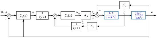
Figure 1.
The permanent magnet synchronous motor (PMSM) speed closed-loop control system.
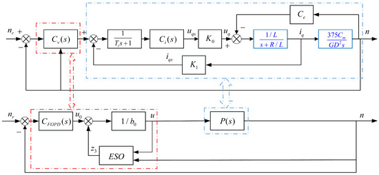
Figure 2.
The PMSM speed closed-loop control system with fractional-order active disturbance rejection control (FOADRC).
Where and n are the reference speed and actual speed, respectively, and the unit is , and are the q-axis current and voltage, respectively, is the induced electromotive force coefficient, and are the voltage and current conversion factors, respectively, is the filter time constant, R and L are the stator equivalent resistance and inductance, respectively, is the torque constant, is the flywheel inertia, and the unit is N·m; is the output of the FOPD controller, is the output of the ESO, and u is the control law.
Assume that hysteresis and eddy current loss, saturation nonlinear factor of magnetization curve and friction are ignored, and there is no damper winding on the rotor. The transfer functions of the electromagnetic and mechanical parts, which are needed to be identified, are shown with zero initial conditions,
A nonlinear identification method based on output-error is adopted to obtain the model parameters [37,38]. Thus, the electromagnetic and mechanical models can be identified as:
The comparison between simulation results based on the obtained models of the electromagnetic and mechanical parts and experimental results are presented in Figure 3 and Figure 4. For more details on the system identification scheme, the reader may refer to Reference [38].
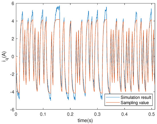
Figure 3.
Actual system output and model output of the electromagnetic part.
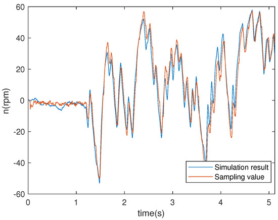
Figure 4.
Actual system output and model output of the mechanical part.
A PI controller with is applied to control the current-loop system,
Based on the above identification results, the speed servo plant of PMSM can be obtained:
where , , U is the input reference current, and Y is the actual speed.
2.4. The Structure of the FOADRC
In this paper, a FOADRC with a FOPD controller is proposed. The structure of the FOADRC is shown in Figure 2.
The load disturbance d is considered when the PMSM is running. Thus, Equation (10) can be rewritten as (11), considering the external disturbance d:
where u and y are the input and output, respectively, d is the external disturbance, and f is the total disturbance, which contains the internal dynamics and external disturbance d.
The FOADRC includes a FOPD controller and an ESO. The ESO of the FOADRC is used to estimate the total disturbance f. Suppose that f is differentiable, , then the state space form of (11) is:
where
Then, the ESO is designed for (12),
where is the gain of the ESO; , , , and are the outputs of the ESO: and will estimate y and its derivative, and will estimate total disturbance f. The estimated total disturbance will be rejected as
where is the output of the FOPD controller.
The FOPD controller is:
where and are the proportional and derivative gains, and is the derivative order.
3. Stability Boundary Analysis
Because the stability is the minimal requirement for the control system, it is desirable to determine the complete stabilizing FOPD parameters before controller design.
In this way, all three of the observer poles will be placed at , which is the observer bandwidth [6].
According to (10), (14) and (16), the plant with disturbance compensation is
where is the Laplace transform of .
In the considered feedback control system as shown in Figure 5, is the controlled plant, and is the designed FOPD controller. There are four tuning parameters: , , , and .
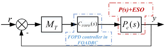
Figure 5.
The PMSM speed closed-loop control system based on FOADRC.
In Figure 5, is a Gain-Phase Margin Tester,
where A and are the gain margin and phase margin, respectively.
The closed-loop transfer function of the control system in Figure 5 can be obtained as:
Hence, the characteristic equation of is:
The range of the fractional-order is defined as . The lower limit of depends on the pre-specified gain crossover frequency , and the upper limit of is set to in this paper. The boundaries of the stable region which are determined by real root boundary (RRB), infinite root boundary (IRB) and complex root boundary (CRB) can be obtained by the D-decomposition method [39,40].
- Real root boundary (RRB): The RRB is defined by the equation , so the boundary of is:
- Infinite root boundary (IRB): Due to the relative order of is 2, has no boundary restrictions.
So, given a fixed fractional-order and a fixed , the stable and unstable regions in the parameter plane can be separated according to the RRB and CRB with , .
One example is given as: Choosing and , draw the curve of w.r.t. and the line according to CRB and RRB, respectively. Detect the stable region by testing a random point [41] as shown in Figure 6. Sweeping all the , the global stable region can be obtained as shown in Figure 7. Thus, with different , different global stable regions can be determined.
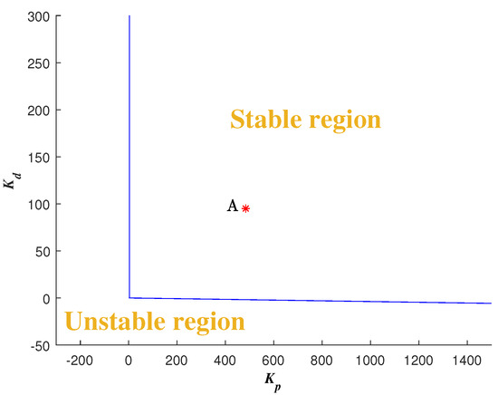
Figure 6.
Stable region with , and the designed and with , .
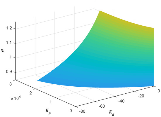
Figure 7.
Global stable region with .
4. FOADRC/IOADRC Design Strategy
4.1. Controller Design Specifications
In this paper, two frequency-domain specifications, gain crossover frequency () and phase margin (PM), are applied to tune FOADRC:
- Gain crossover frequency
- Phase margin
To achieve an optimal dynamic control performance, a time-domain specification, ITAE, is also applied for the FOADRC design:
- ITAEwhere is the deviation between the reference input and the actual output.
4.2. The Optimal FOADRC Design for PMSM Speed Servo Plant
4.2.1. The FOADRC Satisfying the Frequency-Domain Specifications
The Gain-Phase Margin Tester can provide information for satisfying the given gain margin or phase margin [40]. Setting and , plot the curve according to Equations (26) and (27) with increasing from 0. Every point on the above curve fulfills the given phase margin .
The characteristic equation of Equation (20) is,
which denotes the open-loop transfer function equals to ,
so one can get the magnitude and the phase equations,
Thus, all the satisfying (23) can be treated as the gain crossover frequencies with and for the system (18) in Figure 5. Because equations (23) and (32) are equivalent, every frequency corresponding to the point on the curve of versus in parameter plane () can also be treated as .
Thus, with the specified , , a fixed and a fixed , the other two FOADRC parameters and can be determined at a point. Besides, the point should be tested whether it is in the stable region. Then, sweeping over the , a curve in the (, , )-space can be determined. All the points on this curve can be guaranteed to satisfy the two specifications and . Then, Sweeping all the , one can obtain a three-dimensional graph about , and . Every point on this graph corresponding to the parameters () of the FOADRC satisfying the pre-specified and .
One example is given as: With the pre-specified , and fixed , , the point corresponding to the parameters () is determined as a red star ’A’ shown in Figure 6. Sweeping all the in , a series red stars can be obtained shown in Figure 8 and visualized in three-dimensional parameter space which is shown in Figure 9. Every point on this curve meets and according to Figure 10 with the , simultaneously. Sweeping all the in (, 800), one can obtain a three-dimensional scatter plot of as shown in Figure 11. Every point corresponding to the parameters satisfies the frequency-domain specifications and .
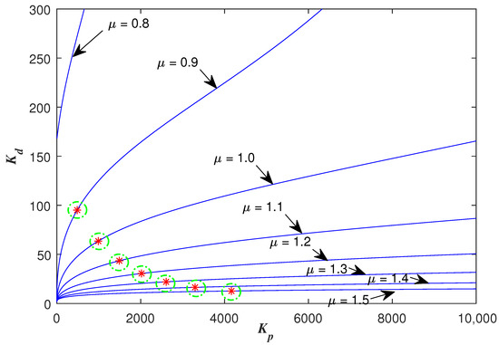
Figure 8.
The designed and with sweeping all the optional .
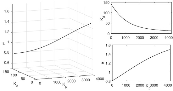
Figure 9.
The designed and with all the .
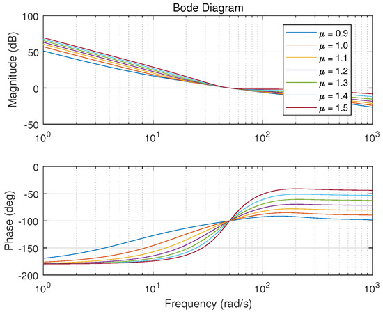
Figure 10.
Bode plots with different .
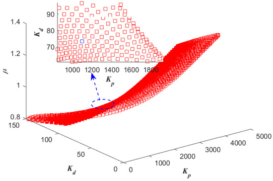
Figure 11.
All the , , and with and .
4.2.2. The Optimal FOADRC Satisfying Time-Domain Specifications
Given all the parameters of the FOADRC corresponding to the point on the above curve in Figure 9, the step and load-disturbance response simulation are implemented and the ITAE of the trial is calculated in MATLAB/Simulink. The ITAE is calculated using (33), which is the sampling form of (30)
Thus, one can obtain the correspondence plot between and as shown in Figure 12. And the smallest corresponding to the is shown as a red star in Figure 12. Sweeping all the in (, 800), the three-dimensional scatter plot of is shown in Figure 13. According to Figure 13, the smallest can be determined, and the parameters () of the optimal FOADRC corresponding to the can be obtained.
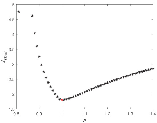
Figure 12.
with different .
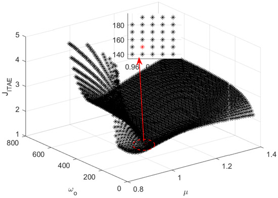
Figure 13.
All the , , and with and .
In summary, the design guidelines are shown in Figure 14.
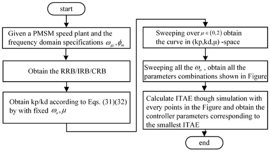
Figure 14.
The design guidelines summary.
4.3. IOADRC Design Strategy
The design strategy for IOADRC satisfying the user-specified frequency specifications and PM is also given with a short explanation. For a fair comparison with FOADRC, set the same with FOADRC. Just as analyzed above, the parameters and with can be determined according to Equations (26) and (27), with , .
5. Simulation Results
In this section, simulation studies are carried out on PMSM speed servo system compared with IOADRC and typical PID controller [42]. The tuning strategy for typical PID controller is based on the frequency-domain specifications (gain crossover frequency, phase margin and flat phase constraint).
5.1. Tracking Performance
Given the frequency-domain specifications and , the optimal FOADRC is obtained applying the above proposed method in Section 4,
For fair comparison, the IOADRC is designed with the same frequency-domain specifications and and the same according to the Section 4.3, so that one can get
Similarly, the typical PID controller can be designed with the same frequency-domain specifications as
The open-loop Bode plots of the three control systems are presented in Figure 15. Three control systems have the same and . The closed-loop Bode plots of three control systems are shown in Figure 16. Figure 16 shows that the designed IOADRC control system has the biggest resonance peak, which means the IOADRC control system has the biggest overshoot than other control systems. The designed PID control system has the smallest overshoot with the smallest resonance.
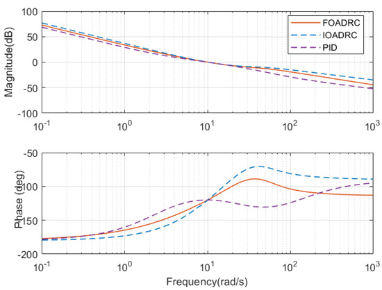
Figure 15.
Open-loop Bode diagrams of three control systems.
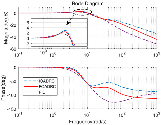
Figure 16.
Closed-loop Bode diagrams of three control systems.
Given the reference speed as , PMSM speed responses are performed, using the designed FOADRC, IOADRC, and PID controller. The simulation results are shown in Figure 17 and Figure 18. The comparison results are shown in Table 1.
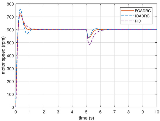
Figure 17.
The speed and anti-load disturbance responses of three control systems (simulation).
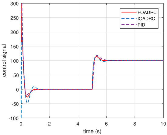
Figure 18.
Control signals of three control systems.

Table 1.
Comparison results of three control systems (simulation).
Obviously, the designed PID control system has the smallest overshoot and the designed FOADRC control system has the biggest overshoot. The overshoots of three control systems are consistent with the analysis in Figure 16. However, comparing with the IOADRC control system, the designed FOADRC control system has shorter settling time () and smaller overshoot (); comparing with PID control system, the designed FOADRC control system has a shorter settling time, although the overshoot is bigger. Overall, the designed FOADRC control system achieves the best tracking performance by comparison with and can achieve a compromise between overshoot and settling time.
5.2. Robustness to External Disturbance
The process sensitivity Bode plots () for three control systems are shown in Figure 19. Figure 19 shows that the designed FOADRC and IOADRC control systems have similar anti-load performance, and both outperform PID control system. Injecting the load disturbance when the motor speed is running, the anti-load disturbance responses of three control systems are performed as shown in Figure 17, and the comparison results are shown in Table 1.
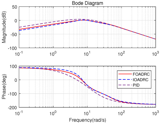
Figure 19.
Sensitivity Bode diagrams of three control systems.
As shown in Figure 19, the designed FOADRC and IOADRC control systems have the similar speed drop, and both are less than the speed drop of the PID control system. According to Figure 17 and Table 1, the designed PID control system has the biggest speed drop () and recovery time; the speed drop shows that the anti-load disturbance performances of FOADRC and IOADRC control systems are basically the same and both significantly smaller than the PID control system, which also can be seen clearly from . These results are consistent with the analysis from Figure 19.
6. Experiment Results and Discussion
In this section, the real PMSM speed control experiments are carried out to verify the effectiveness of the proposed tuning strategy for FOADRC and IOADRC. The laboratory PMSM platform is shown in Figure 20. The platform consists of a PMSM, which the model is Sanyo-P50B08075HXS, a DC generator, a DC power, a servo driver, and a PC. The servo drive is based on the TMS320F28335 DSP and control algorithm implementation based on C-program. The sampling frequency of the current-loop is 8 and the velocity-loop is 1.6. The fractional-order operator is implemented by the impulse-response-invariant-discretization (IRID) method [36] and has the following form (Equation (37)), with the sampling period , and the comparison of approximated Bode plot and true Bode plot is shown in Figure 21.
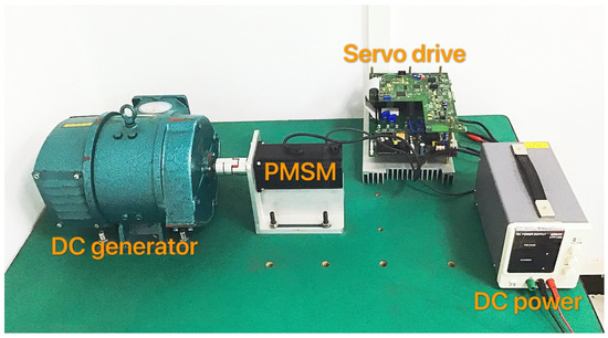
Figure 20.
The PMSM speed control platform
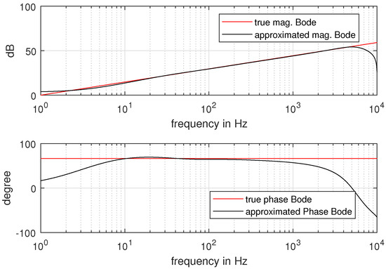
Figure 21.
Comparison of approximated Bode plot and true Bode plot.
6.1. Tracking Performance
Setting the reference speed as 600 , PMSM speed step response experiments are performed, using the designed FOADRC, IOADRC, and PID controller. The experimental results are presented in Figure 22, and the comparison results are shown in Table 2.
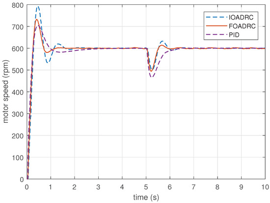
Figure 22.
The speed and anti-load disturbance responses of three control systems (experiment).
Table 2.
Comparison results of three control systems (experiment).
Figure 22 shows that the designed PID control system has the smallest overshoot, and the designed IOADRC control system achieves the biggest overshoot, which are consistent with the analysis from Figure 16 and the simulation results in Figure 17. Comparing with the IOADRC control system, the designed FOADRC control system has shorter settling time (0.985) and smaller overshoot (22.1%); the designed PID control system has the smallest overshoot but the longest settling time. In summary, the FOADRC control system achieves the best tracking performance according to the and can achieve a compromised performance in terms of overshoot and settling time between IOADRC and PID control systems.
6.2. Robustness to External Disturbance
Rejecting the same disturbance, the anti-load disturbance responses of three control systems are performed in Figure 22. As can be seen visually from Figure 22, IOADRC and FOADRC control systems achieve the similar speed drop and both less than the speed drop of the PID control system. There result are consistent with the analysis from Figure 19 and the simulation results in Figure 17. The designed PID control system has the biggest speed drop () and recovery time. The IOADRC and FOADRC control systems have basically similar speed drop ( and ), and the anti-load disturbance performance of IOADRC has a little oscillation. The detailed comparison results are shown in Table 2. In summary, the proposed FOADRC can achieve the best control performance in terms of anti-load over IOADRC and PID controller.
6.3. Discussion
Comparing with the traditional IOADRC, the proposed FOADRC can achieve better tracking performance with a smaller overshoot, and the value of the is smaller. On the other hand, the proposed FOADRC has a little bigger speed drop when inputs load comparing with IOADRC. However, recover time is less than IOADRC and has a smaller value of . Comparing with the traditional PID controller, the proposed FOADRC can achieve better disturbance rejection performance with less speed drop when inputs load. On the other hand, the proposed FOADRC has a bigger overshoot comparing with PID controller. However, the settling time of the proposed FOADRC is less than the one of PID controller and has less .
7. Conclusions
The paper proposes a FOADRC with a FOPD controller for the PMSM speed servo system, which is identified through a nonlinear identification method. A stabilization method is presented to obtain the stabilizing FOPD controller for the PMSM speed servo plant via D-decomposition. Furthermore, a synthesis is proposed for the FOADRC design to meet user-specified frequency-domain specifications, i.e., phase margin and gain crossover frequency, and the time-domain specification, i.e., ITAE, simultaneously. The design method is also applicable to IOADRC. The designed optimal FOADRC/IOADRC can get desired control performance as satisfying two given frequency-domain specifications and the optimal . The simulation and experiment are carried out for the PMSM speed servo, comprised of the traditional IOADRC and PID controller. Based on the simulation and experiment results, the proposed FOADRC can achieve better tracking performance and more robustness to external disturbance. The for speed tracking of the designed FOADRC are 52.59% and 55.36% better than the of IOADRC and PID controller, respectively. Obviously, the settling time of the designed FOADRC is the shortest (0.7369 s), which is 32.99% and 49.22% less than the settling time of the designed IOADRC and PID controller. Besides, the for anti-load disturbance of the designed FOADRC is 17.11% and 52.50% better than the of IOADRC and PID controller, respectively.
Author Contributions
Conceptualization, Y.L.; Data curation, P.C.; Formal analysis, P.C.; Funding acquisition, Y.L.; Investigation, P.C. and Y.L.; Methodology, Y.L.; Project administration, Y.L.; Resources, Y.L. and Y.P.; Software, P.C.; Supervision, Y.L.; Validation, P.C.; Visualization, Y.P. and Y.C.; Writing—original draft, P.C.; Writing—review & editing, Y.L. and Y.C. All authors have read and agreed to the published version of the manuscript.
Funding
This research was funded by National Natural Science Foundation of China [51975234].
Institutional Review Board Statement
Not applicable.
Informed Consent Statement
Not applicable.
Data Availability Statement
Date sharing not applicable.
Conflicts of Interest
The authors declare no conflict of interest.
Abbreviations
| fractional-order active disturbance rejection control | |
| fractional-order proportional-derivative | |
| extended state observer | |
| permanent magnet synchronous motor | |
| active disturbance rejection control | |
| integer-order active disturbance rejection control | |
| proportional-integral-derivative | |
| fractional-order | |
| fractional-order proportional-integral | |
| fractional-order (proportional-derivative) | |
| fractional-order proportional-integral-derivative | |
| integral square error | |
| integral time absolute error | |
| linear active disturbance rejection control | |
| generalized active disturbance rejection control | |
| genetic algorithm | |
| fractional active disturbance rejection control | |
| fractional-order extended state observer | |
| fractional order system | |
| proportional-integral | |
| real root boundary | |
| infinite root boundary | |
| complex root boundary | |
| phase margin | |
| impulse-response-invariant-discretization |
References
- Krishnan, R. Electric Motor Drives: Modeling, Analysis, and Control; Prentice Hall: Upper Saddle River, NJ, USA, 2001. [Google Scholar]
- Alcántara, S.; Vilanova, R.; Pedret, C. PID control in terms of robustness/performance and servo/regulator trade-offs: A unifying approach to balanced autotuning. J. Process Control 2013, 23, 527–542. [Google Scholar] [CrossRef]
- Han, J. From PID to active disturbance rejection control. IEEE Trans. Ind. Electron. 2009, 56, 900–906. [Google Scholar] [CrossRef]
- Horowitz, I.M. Synthesis of Feedback Systems; Elsevier: Amsterdam, The Netherlands, 2013. [Google Scholar]
- Tsien, H.S. Engineering Cybernetics; McGraw-Hill: New York, NY, USA, 1954. [Google Scholar]
- Gao, Z. Scaling and bandwidth-parameterization based controller tuning. Proc. Am. Control. Conf. 2006, 6, 4989–4996. [Google Scholar]
- Xue, W.; Bai, W.; Yang, S.; Song, K.; Huang, Y.; Xie, H. ADRC with adaptive extended state observer and its application to air–fuel ratio control in gasoline engines. IEEE Trans. Ind. Electron. 2015, 62, 5847–5857. [Google Scholar] [CrossRef]
- Zheng, Q.; Gao, Z. On practical applications of active disturbance rejection control. In Proceedings of the 29th Chinese Control Conference, Beijing, China, 29–31 July 2010; pp. 6095–6100. [Google Scholar]
- Wenchao, H.Y.X. Active disturbance rejection control: Methodology, applications and theoretical analysis. J. Syst. Sci. Math. Sci. 2012, 32, 1287–1307. [Google Scholar]
- Wu, Z.; He, T.; Li, D.; Xue, Y.; Sun, L.; Sun, L. Superheated steam temperature control based on modified active disturbance rejection control. Control Eng. Pract. 2019, 83, 83–97. [Google Scholar] [CrossRef]
- Fu, C.; Tan, W. Tuning of linear ADRC with known plant information. ISA Trans. 2016, 65, 384–393. [Google Scholar] [CrossRef] [PubMed]
- Zhou, X.; Gao, H.; Zhao, B.; Zhao, L. A GA-based parameters tuning method for an ADRC controller of ISP for aerial remote sensing applications. ISA Trans. 2018, 81, 318–328. [Google Scholar] [CrossRef]
- Oldham, K.B.; Spanier, J. The fractional calculus. Math. Gaz. 1974, 56, 396–400. [Google Scholar]
- Ross, B. The development of fractional calculus 1695–1900. Hist. Math. 1977, 4, 75–89. [Google Scholar] [CrossRef]
- Freeborn, T.J. A survey of fractional-order circuit models for biology and biomedicine. IEEE J. Emerg. Sel. Top. Circuits Syst. 2013, 3, 416–424. [Google Scholar] [CrossRef]
- Vastarouchas, C.; Dimeas, I.; Psychalinos, C.; Elwakil, A.S. Fractional Order Systems; Chapter 6. Fractional-Order Integrated Circuits in Control Applications and Biological Modeling; Elsevier: Amsterdam, The Netherlands, 2018; pp. 163–204. [Google Scholar]
- Abdou, M. On the fractional order space-time nonlinear equations arising in plasma physics. Indian J. Phys. 2019, 93, 537–541. [Google Scholar] [CrossRef]
- Luo, Y.; Chen, Y. Fractional Order Motion Controls; Wiley Online Library: Hoboken, NJ, USA, 2012. [Google Scholar]
- Mescia, L.; Bia, P.; Caratelli, D. Fractional-Calculus-Based Electromagnetic Tool to Study Pulse Propagation in Arbitrary Dispersive Dielectrics. Phys. Status Solidi A 2019, 216. [Google Scholar] [CrossRef]
- Wang, C.; Luo, Y.; Chen, Y. Fractional order proportional integral (FOPI) and [proportional integral](FO[PI]) controller designs for first order plus time delay (FOPTD) systems. In Proceedings of the 21st Chinese Control and Decision Conference (CCDC), Guilin, China, 17–19 June 2009; pp. 329–334. [Google Scholar]
- Zheng, W.; Luo, Y.; Pi, Y.; Chen, Y. Improved frequency-domain design method for the fractional order proportional–integral–derivative controller optimal design: A case study of permanent magnet synchronous motor speed control. IET Control Theory Appl. 2018, 12, 2478–2487. [Google Scholar] [CrossRef]
- Luo, Y.; Chen, Y. Fractional order [proportional derivative] controller for a class of fractional order systems. Automatica 2009, 45, 2446–2450. [Google Scholar] [CrossRef]
- Vinagre, B.M.; Monje, C.A.; Calderon, A.J.; Suarez, J.I. Fractional PID controllers for industry application. A brief introduction. J. Vib. Control 2007, 13, 1419–1429. [Google Scholar] [CrossRef]
- De Keyser, R.; Muresan, C.I.; Ionescu, C.M. A novel auto-tuning method for fractional order PI/PD controllers. ISA Trans. 2016, 62, 268–275. [Google Scholar] [CrossRef] [PubMed]
- Biswas, A.; Das, S.; Abraham, A.; Dasgupta, S. Design of fractional-order PID controllers with an improved differential evolution. Eng. Appl. Artif. Intell. 2009, 22, 343–350. [Google Scholar] [CrossRef]
- Zeng, G.Q.; Chen, J.; Dai, Y.X.; Li, L.M.; Zheng, C.W.; Chen, M.R. Design of fractional order PID controller for automatic regulator voltage system based on multi-objective extremal optimization. Neurocomputing 2015, 160, 173–184. [Google Scholar] [CrossRef]
- Monje, C.A.; Vinagre, B.M.; Feliu, V.; Chen, Y. Tuning and auto-tuning of fractional order controllers for industry applications. Control Eng. Pract. 2008, 16, 798–812. [Google Scholar] [CrossRef]
- Luo, Y.; Zhang, T.; Lee, B.J.; Kang, C.; Chen, Y.Q. Fractional-Order Proportional Derivative Controller Synthesis and Implementation for Hard-Disk-Drive Servo System. IEEE Trans. Control Syst. Technol. 2014, 22, 281–289. [Google Scholar] [CrossRef]
- Li, H.S.; Luo, Y.; Chen, Y.Q. A Fractional Order Proportional and Derivative (FOPD) Motion Controller: Tuning Rule and Experiments. IEEE Trans. Control Syst. Technol. 2010, 18, 516–520. [Google Scholar] [CrossRef]
- Li, D.; Ding, P.; Gao, Z. Fractional active disturbance rejection control. ISA Trans. 2016, 62, 109–119. [Google Scholar] [CrossRef] [PubMed]
- Shi, X.; Chen, Y.; Huang, J. Application of fractional-order active disturbance rejection controller on linear motion system. Control Eng. Pract. 2018, 81, 207–214. [Google Scholar] [CrossRef]
- Chen, P.; Luo, Y.; Zheng, W.; Gao, Z. A New Active Disturbance Rejection Controller Design Based on Fractional Extended State Observer. In Proceedings of the 38th Chinese Control Conference (CCC), Guangzhou, China, 27–30 July 2019; pp. 4276–4281. [Google Scholar]
- Sun, B.; Gao, Z. A DSP-based active disturbance rejection control design for a 1-kW H-bridge DC-DC power converter. IEEE Trans. Ind. Electron. 2005, 52, 1271–1277. [Google Scholar] [CrossRef]
- Ahi, B.; Haeri, M. Linear Active Disturbance Rejection Control From the Practical Aspects. IEEE/ASME Trans. Mech. 2018, 23, 2909–2919. [Google Scholar] [CrossRef]
- Nowak, P.; Czeczot, J.; Klopot, T. Robust tuning of a first order reduced Active Disturbance Rejection Controller. Control Eng. Pract. 2018, 74, 44–57. [Google Scholar] [CrossRef]
- Chen, Y. Impulse Response Invariant Discretization of Fractional Order Integrators/Differentiators, Filter Design and Analysis, MATLAB Central. Available online: http://www.mathworks.com/matlabcentral/fileexchange/21342impulse-response-invariant-discretization-of-fractional-order-integrators-differentiator (accessed on 20 February 2021).
- Poinot, T.; Trigeassou, J.C. Identification of fractional systems using an output-error technique. Nonlinear Dyn. 2004, 38, 133–154. [Google Scholar] [CrossRef]
- Zheng, W.; Luo, Y.; Chen, Y.; Pi, Y. Fractional-order modeling of permanent magnet synchronous motor speed servo system. J. Vib. Control 2016, 22, 2255–2280. [Google Scholar] [CrossRef]
- Ackermann, J.; Kaesbauer, D. Stable polyhedra in parameter space. Automatica 2003, 39, 937–943. [Google Scholar] [CrossRef]
- Hamamci, S.E. An algorithm for stabilization of fractional-order time delay systems using fractional-order PID controllers. IEEE Trans. Autom. Control 2007, 52, 1964–1969. [Google Scholar] [CrossRef]
- Hwang, C.; Cheng, Y. A numerical algorithm for stability testing of fractional delay systems. Automatica 2006, 42, 825–831. [Google Scholar] [CrossRef]
- Chen, Y.; Moore, K. Relay feedback tuning of robust PID controllers with iso-damping property. IEEE Trans. Syst. 2005, 35, 23–31. [Google Scholar] [CrossRef] [PubMed]
Publisher’s Note: MDPI stays neutral with regard to jurisdictional claims in published maps and institutional affiliations. |
© 2021 by the authors. Licensee MDPI, Basel, Switzerland. This article is an open access article distributed under the terms and conditions of the Creative Commons Attribution (CC BY) license (http://creativecommons.org/licenses/by/4.0/).