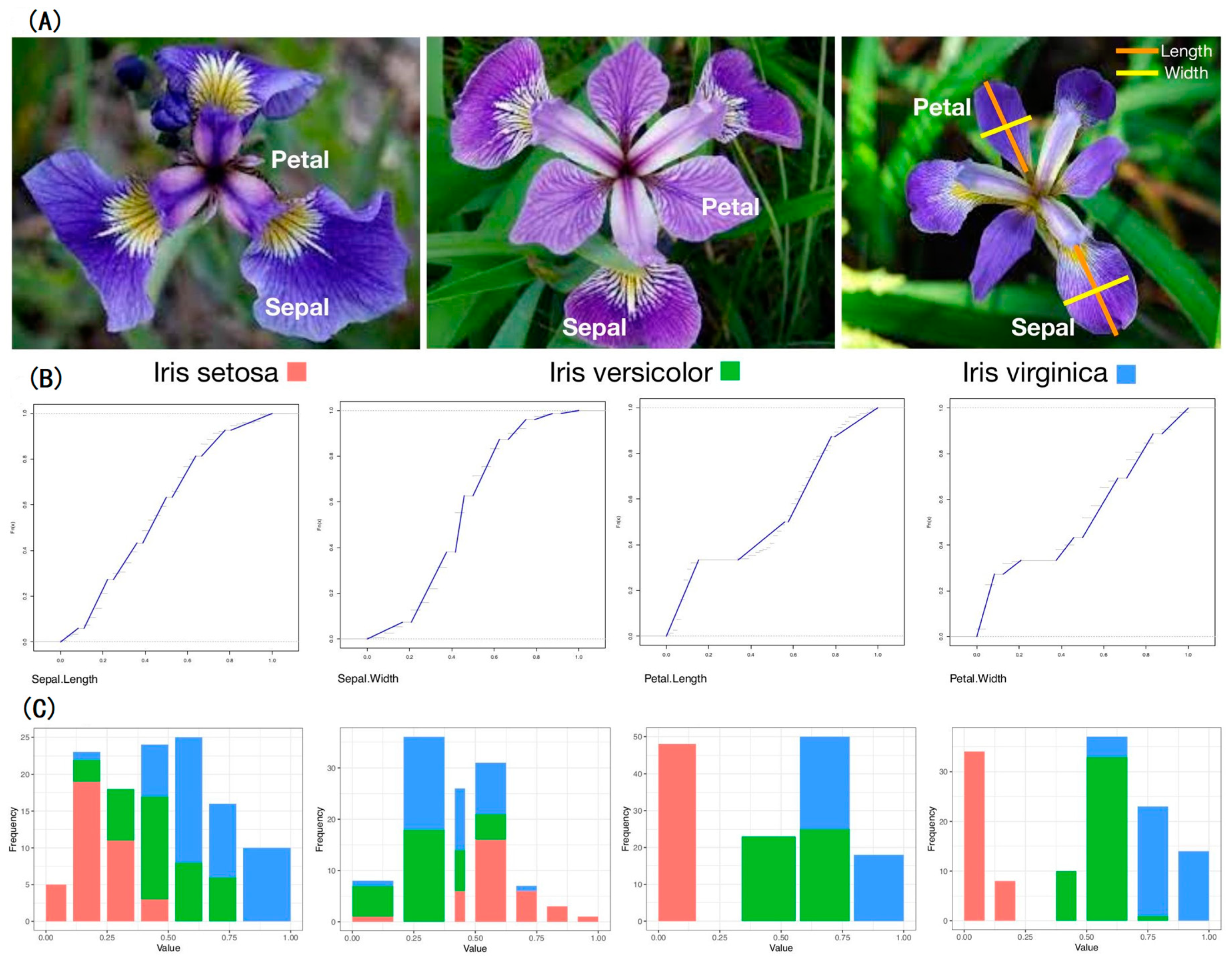
A multiclass classification (MCC) setting can be found in the heart of a majority of real-world complex systems, such as species in nature, diseases in medicine, and pitchers in the MLB. Its collection of labels, called label space, knowingly or unknowingly, capsulizes many defining characteristics of its members through either natural or man-made labeling processes. There are two major types of labeling. One is for structured data, and the other is for unstructured data. For instance, the three Iris images in
Figure 1 are unstructured data, while a 4D vector of measurements of the four features is structured data. Typical examples of unstructured data include images from nature or human activities or articles from newspapers or magazines, or even websites [
12]. Labeling on unstructured data, in general, is subjective. Thus, the MCC information content of any unstructured dataset could vary from one researcher to another.
In sharp contrast, an MCC on a structured dataset is understood as a setting that the data’s curator has knowingly encoded and encapsulated the system-specific knowledge and intelligence by selecting or engineering K features for sufficiently labeling each of N subjects into one of L labels. The MCC information content of a structured dataset is exactly specified by the L labels, K features, and N subjects.
In this section, we want to computationally uncover and decode knowledge and intelligence underlying MCC settings upon a structured dataset. To a great extent, as a reverse engineering endeavor, our CEDA computational developments for MCC should uncover and decode the labeling process. That is, the ultimate goal of CEDA on an MCC is focused on its total information content. This goal has never been explicitly discussed and presented yet in the literature.
4.1. Multiscale Complexity in MCC Information Content
In this section, we consider two structured datasets from PITCHf/x database of two pitch-types: slider and curveball. The MCC information content of each pitch-type specific structured dataset is used to shed lights on questions such as: How can we characterize chief distinctions among MLB pitchers’ pitching dynamics precisely? Can we make such characteristics and distinctions visible and explainable? Is it possible to explain each of our predictive decision-makings with a pattern-based reason? Can we make no mistakes in identifying labels? These questions are essential for understanding each of the two pitch-type specific pitching dynamic systems.
When L, K, and ), the total number of data points are not too small, and such MCC information content indeed can be rather complex. One way of perceiving such complexity is through a mixing geometry of all labels’ point-clouds determined by a subset of k (≤K) features. Such a mixing geometry indeed can exhibit potentially non-linear associative relations among the k features because their associations shape each label’s k-dimensional point-cloud individually and in turn dictate the global mixing geometry among all point-clouds collectively.
If one feature-set offers one perspective of mixing geometry, then there are possible feature-sets. Thus, there are too many and too diverse candidate perspectives of MCC information content to be examined and chosen from. Further, due to temporal and spatial separations, these non-linear feature-to-feature associations are likely directed, so their geometric mixing patterns indeed are likely asymmetric. That is, views of one single mixing geometry can vary according to different point-clouds standpoints. As shown below, such hardly known mixing geometric asymmetry indeed helps us to see through the complexity of MCC information content, if we carefully choose which perspectives to look into.
We make use of such asymmetric mixing geometry of point-clouds to formulate the concept of complementary feature-sets. The rationale is given as follows. If a mixing geometry of one feature-set shows clear separations among a sub-group of pitchers’ point-clouds, but at the same time reveals intense mixing among another subgroup of pitchers’ point-clouds, then we would like to identify a mixing geometry of a complementary feature-set that could reveal the opposite mixing patterns. By identifying such a pair of complementary feature-sets, we can arrange them into a chain so that the uncertainty caused by mixing among point-clouds of the first feature-set can be significantly mitigated and even minimized due to different perspective views provided by the latter feature-set. Likewise, we can build a chain of three feature-groups if it is necessary. As demonstrated below, the order of feature-groups is critical in building up such a chain. A well-constructed chain of complementary feature-groups would give rise to a collection of serial patterns of mixing geometry to constitute the essential and brand new aspects of full MCC information content.
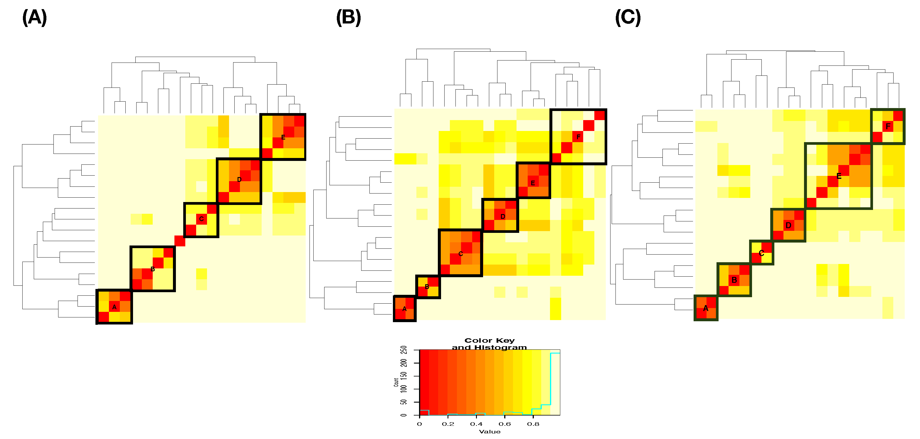
At this stage of knowledge, exploratory data analysis (EDA) could be the only computationally feasible way of discovering complementary feature-sets under an MCC setting. How to efficiently explore and discover an effective chain becomes an essential computational issue. On top of this exploring issue, another issue is how to concisely present synthesized serial pattern information from complementary feature-sets. To resolve both issues, we turn to the road-map provided by a heatmap of the
MCE matrix among
K features, as illustrated in
Figure 3. Due to the categorical nature of MCE, we term our data-driven explorations and computational developments the categorical exploratory data analysis (CEDA) for MCC.
Given that a feature-group specifies a mixing geometry of all point-clouds, our computational developments for CEDA for MCC pertaining to a feature-group would consist of two tasks: (1) building one label embedding tree; and (2) constructing one predictive map. Based on various feature-group specific predictive maps, the third task of our CEDA for MCC is to decide a chain of complementary feature-groups and represent the collection of serial mixing geometric patterns. The procedure of MCC is summarized in Algorithm 1.
![Entropy 23 00792 i001]()
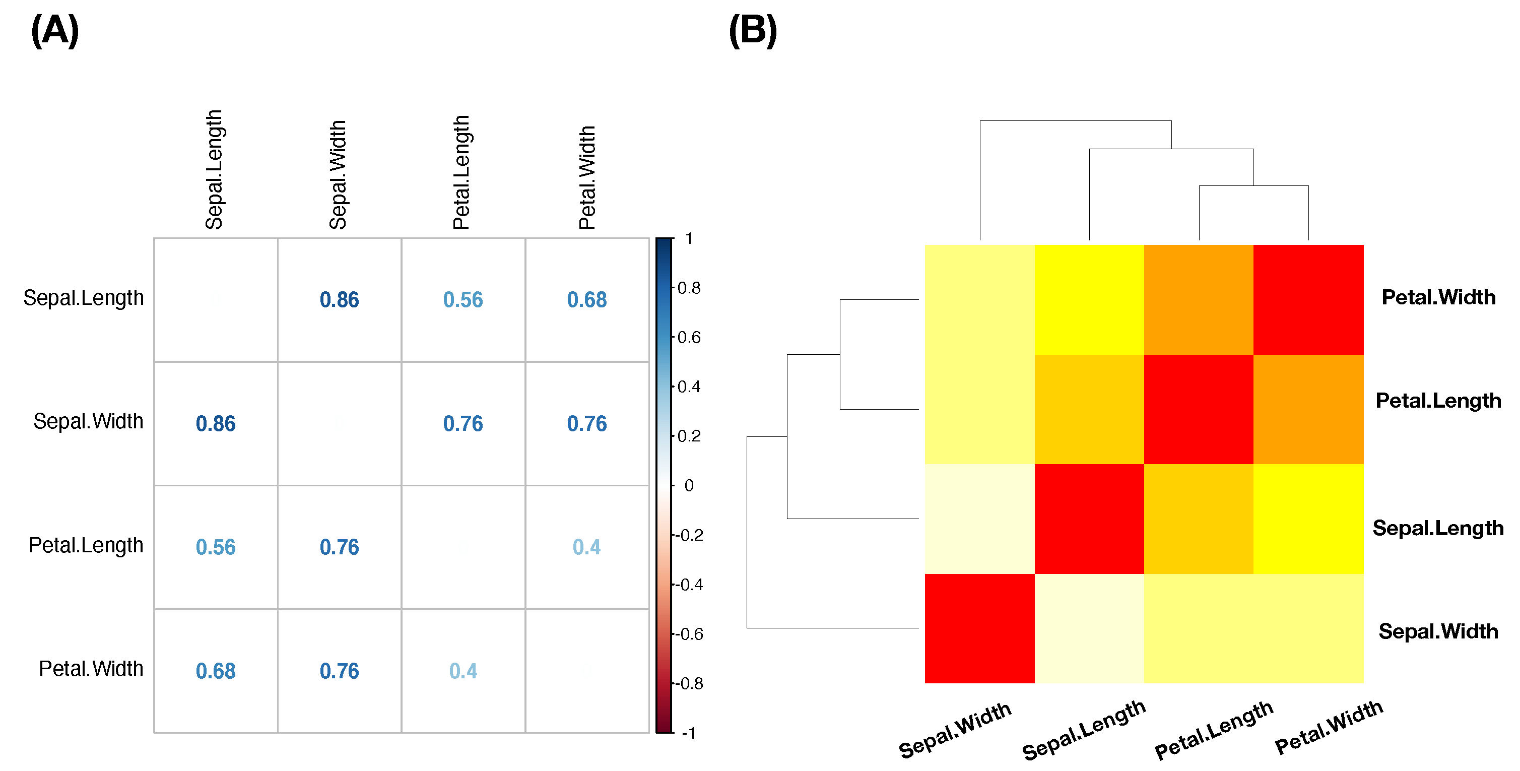
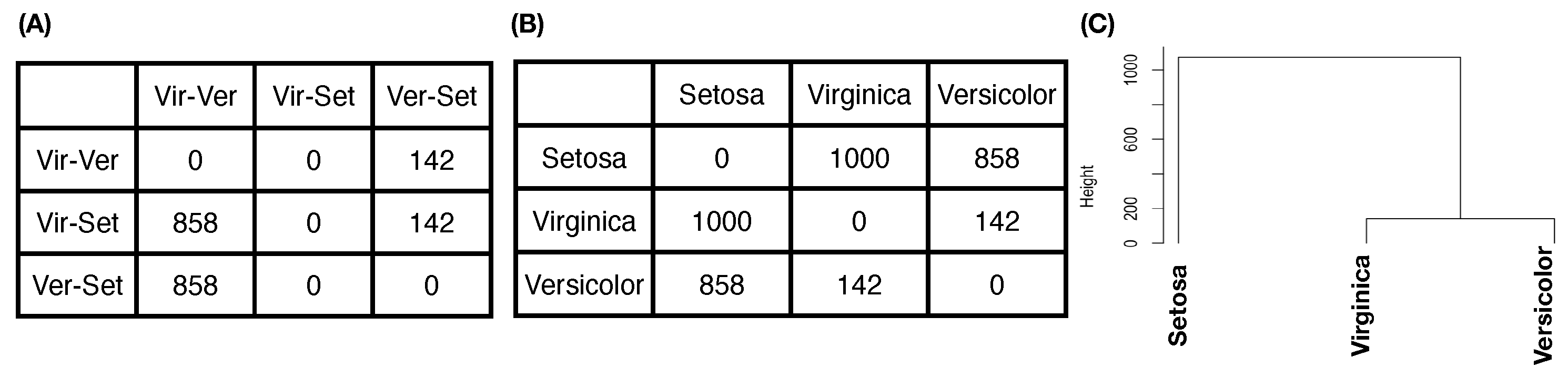
One new and significant computational development of CEDA for MCC is our proposal of “relative distance” between one label’s whole point-cloud and another label’s whole point-cloud. The geometric shapes or distributions of L labels’ k-dimensional point-clouds can be rather distinct. Such heterogeneity in geometric shape is rather difficult to be accommodated well in any direct distance measure. In other words, all direct distance measures are non-robust with respect to variations on edges of point-clouds, such as optimal transport. To robustly mitigate such edge effect, we propose a new concept of relative distance. We consider a triplet of labels’ point-clouds and intend to evaluate which two labels’ of point-clouds are closer than each of them to the third label’s point-cloud. That is, we consider “dominance”, not distance. Such closeness-based dominance is explicitly evaluated in the following collective fashion. We randomly select one k-dimensional point from each of the three point-clouds in . We calculate the three point-point Euclidean distance in , and record which the two point-point Euclidean distance dominates label-pair’s point-point Euclidean distance. We can perform these triplet competitions for as many runs as we want. For illustrative purpose, we report an experiment on the feature-group (petal-length, petal-width) of Iris data with 1000 triplet competitions.
Figure 6A indicates that, among the 1000 competitions, the first row shows that the pair (Virginica, Versicolor), denoted as Vir-Ver, never dominates Vir-Set, while dominating Ver-Set 142 times. The second row shows that Vir-Set dominates Vir-Ver 858 times and Ver-Set 142 times. The third row shows that Ver-Set dominates Vir-Ver 858 times but never dominates Ver-Set. The vector row sum
shows the order of closeness among the three pairs. In particular, the “relative distance” of Vir-Ver is the smallest to be dominated more than
of the time, while the “relative distance” of Vir-Set is the largest among the three pairwise “relative distances”. That is, we can convert the vector of row sums into a relative distance matrix of the three species of Iris, as shown in
Figure 6B. It is noted that this relative distance matrix is robust with all shapes of three point-clouds [
19]. Then, we can derive a HC-tree based on this relative distance matrix, as shown in
Figure 6C. This HC-tree is called the label-embedding tree (LET) upon the three species.
To ensure that the resultant LET can retain and explicitly reveal full mixing geometry among all involving point-clouds, the training dataset used for such computations usually occupies the majority of the whole dataset. In this paper, we use
of the original dataset as the training dataset for the first task of CEDA for MCC, while the remaining
is the testing dataset. In the second task of CEDA for MCC, each data point in the testing dataset is provided a series of binary competitions that are carried out by descending from the LET’s tree-top to its bottom. By continuing this Iris example with the LET given in
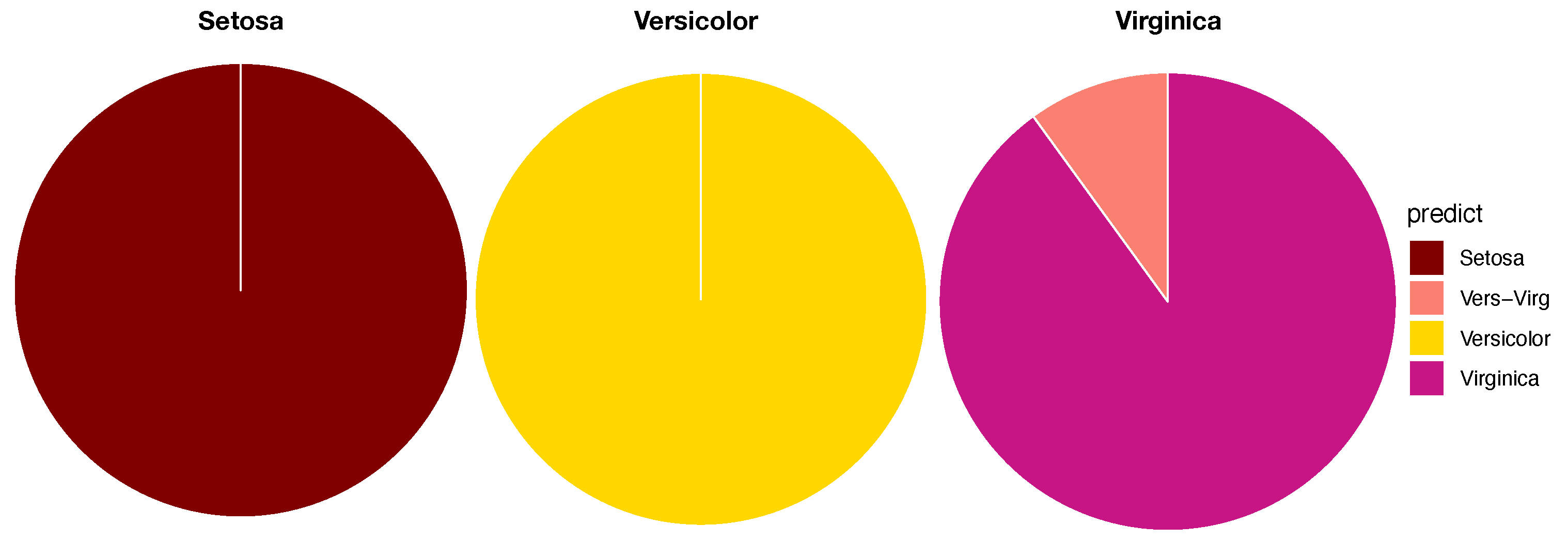
Figure 6C, the first binary (Left-vs.-Right) competition always occurs at the top internal node of the whole LET: Left-branch (Setosa) against Right-branch (Versicolor, Virginaica). If a testing data point is declared belonging to the Left-branch, then the serial competition ends. If it is declared to be in Right-branch, then the second binary competition occurs at the top internal node of the Right-branch: Left-branch (Virginaica) against Right-branch (Versicolor). The decision-making rules of such a binary competition are given in the following subsection. There are three possible outcomes for each binary competition: (1) Left-branch; (2) Right-branch; and (3) both branches. The third outcome is designed for testing data points that are located within localities having complicated mixing patterns. Therefore, the serial competitions will end either at the bottom tree leaf or at an internal node. We use a pie chart to represent the outcomes of such serial binary competitions for testing data points having the same original label. The three resultant pie charts of the Iris example are given in
Figure 7.
As illustrated via the three pie charts in
Figure 7, by using (petal length, petal width) as the feature-group and its three corresponding 2D point-clouds, we can predict Setosa and Versicolor with a singleton predictor without errors. The majority of testing data points of Virginica can also afford a singleton predictor, but some testing data points must be declared with a decision as (Versicolor, Virginaica). This is an evident form of asymmetric mixing geometric pattern (see the top layer of
Table 1).
To mitigate the uncertainty within such asymmetry of mixing geometry, we employ the chain of complementary feature-group. It is natural and logical to couple the feature-group (petal length, petal width) with the feature-group (sepal length, sepal width) to form a chain (petal length, petal width) ⇒ (sepal length, sepal width). The results of this chain of two complementary feature-group are shown via a two-layer table in
Table 1. The effect of using (sepal length, sepal width) feature-group as a complementary feature-group (petal length, petal width) is evident. The uncertainty of Vir-Ver in the pie chart of Versicolor is explained as: this testing data point of Virginica is found close to Versicolor and Virginica, while it is found close to Setosa with respect to the perspective of (sepal length, sepal width). This is the third task of CEDA for MCC for this Iris example. This tabular representation of a collection of serial mixing geometric pattern-categories is the major part of MCC information content.
It is important to note that the ordering of feature-groups in a chain of complementary feature-groups is essential. The first feature-group plays the role of major factor in MCC, while the second and third ones are minor factors. We illustrate the importance of this ordering by computing the performance of a chain of reverse ordering (sepal length, sepal width) ⇒ (petal length, petal width). As shown in the second layers of
Table 2, there are cases with uncertainty.
It is essential to recognize that such a tabular representation explicitly reveals which part of label-specific point-cloud can be perfectly predicted via a singleton-label and which parts are predicted by label-sets. Each pattern-category prescribes an error-free decision. This fact demonstrates that all inferential decisions can be fully supported by visible and explainable MCC information content. If this becomes a well-recognized fundamental standpoint for data analysis, then data analysis would be naturally embedded into scientific research.
In contrast, nowadays, the inference is the primary focus in statistics and machine learning literature [
20,
21,
22]. Such an inferential endeavor usually focuses only on selecting the best feature-set to achieve a man-made criterion, such as minimizing the predictive error rate. Many essential parts of data’s information content pertaining to different feature-groups are ignored. Further, such an inference typically owns a foremost limit of making a singleton-label predictor. It is obvious that data do not fully support such decision-making. The consequences are seen from the following two aspects: (1) data’s pertinent uncertainty is ignored; and (2) statisticians or ML researchers force themselves to make prediction mistakes.
In the following two subsections, we expand and demonstrate our computational developments of CEDA for MCC onto two much more complex MCC settings, slider and curveball, than the illustrative Iris example.
4.2. CEDA for MCC on Slider Data
Here, we reiterate that the slider’s speed is slightly less than the fastball, but much higher than the curveball within a pitcher’s pitching repertoire. Its spin direction (“spin_dir”) has a much wider range than that of both fastball and curveball. Due to the Magnus effect, its horizontal movement (“pfx_x”) is very versatile. A pitcher typically changes spin directions and spin rates and speed to create an extensive range of spectrums of “pfx_x” and vertical movement (“pfx_z”) to effectively deal with batters. Hence, a professional slider pitcher is a wizard of spin and speed. The MCC on silder data is to classify among these “wizards”.
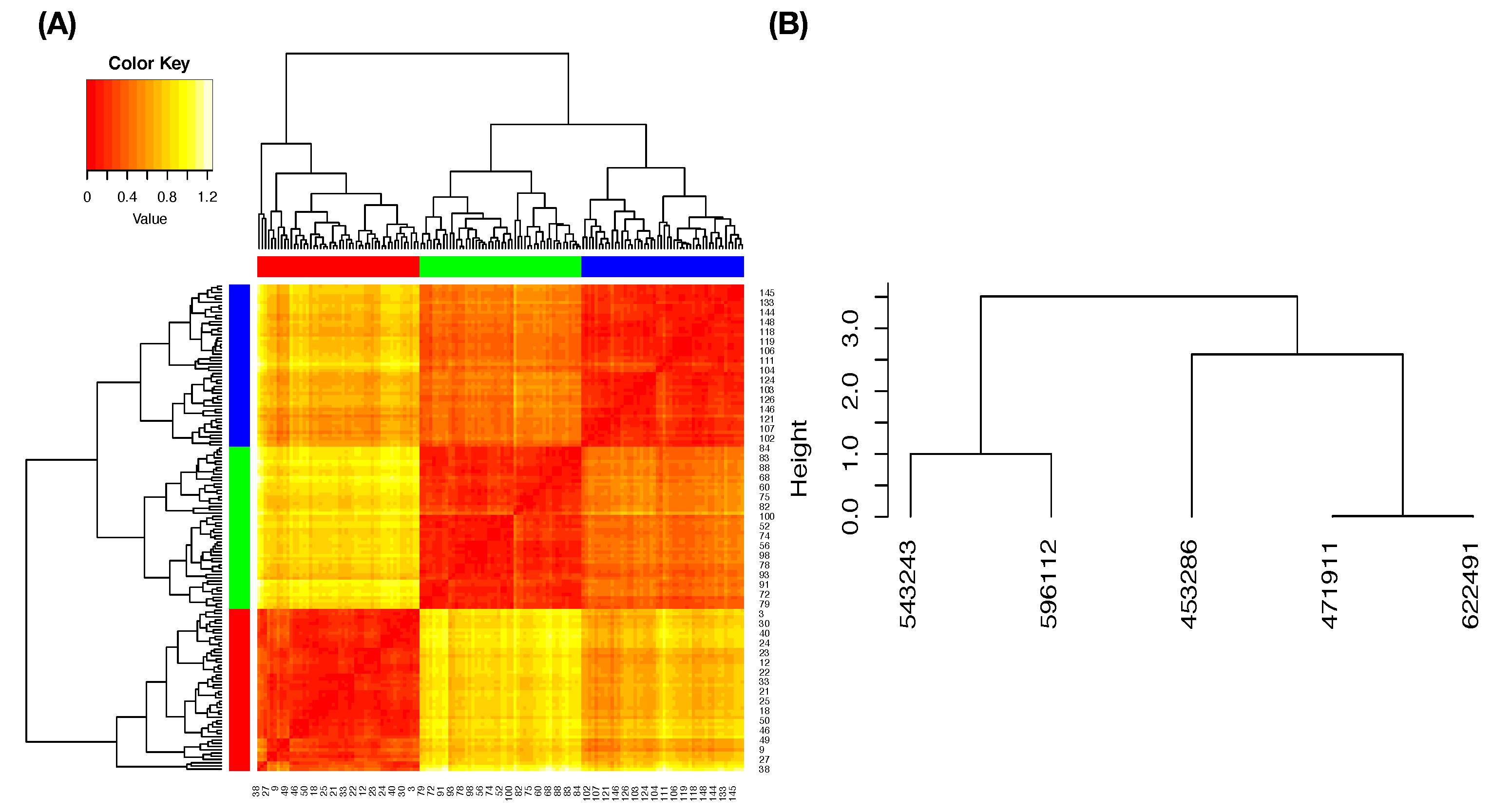
We use a slider dataset consisting of only five
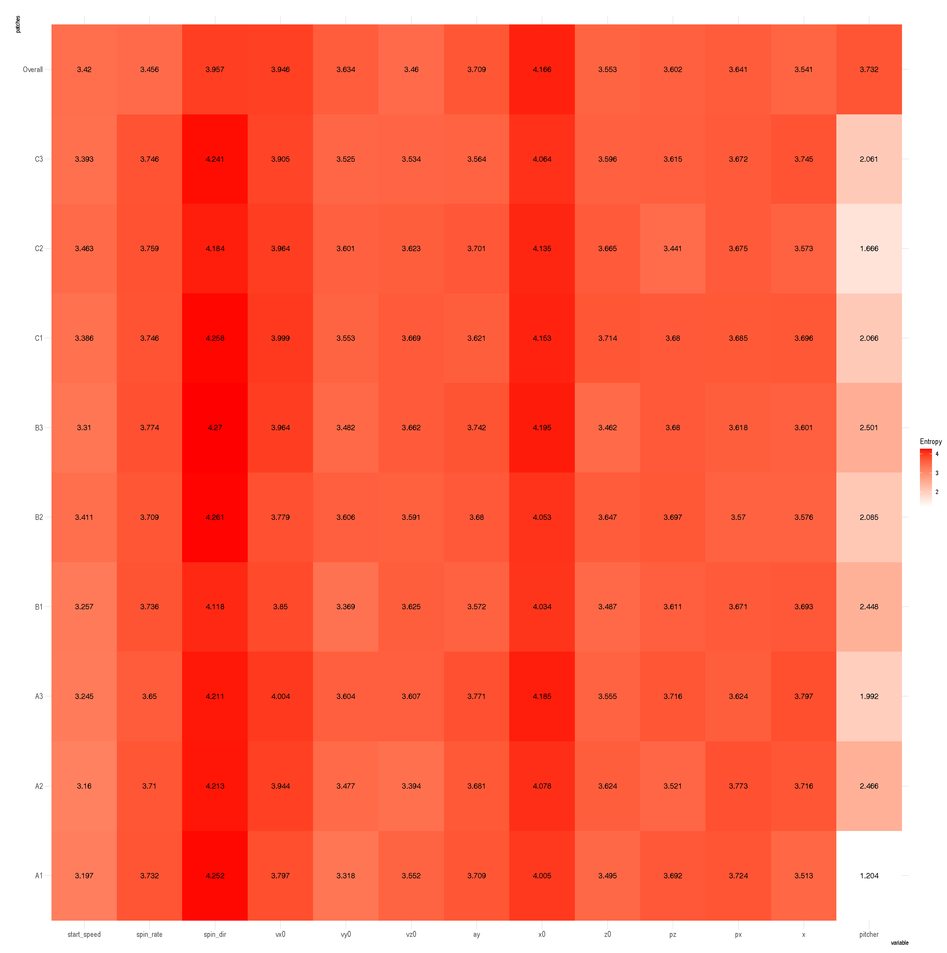
MLB pitchers from the 2017 season to demonstrate our CEDA for MCC computing. Here, we take a MLB pitcher-ID as a label of his slider pitches. The slider’s mutual conditional entropy matrix, as shown in
Figure 4A, clearly reveals five evident blocks as marked along its diagonal. These five highly associated feature-groups with memberships are listed as follows: Group A, {“end_speed”, “start_speed”, “vyo”}; Group B, {“px”, “x”, “vz0”, “pz”}; Group C, {“z0”, “vx0”, “x0”}; Group D, {“spin_dir”, “break_angle”, “ax”, “pfx_x”}; and Group E, {“spin_rate”, “break_length”, “pfx_z”,“az”}. If we take each synergistic feature-group as a mechanical entity, we have achieve the “dimension reduction” from
to 5. Via directed associations from pitcher-ID, we find the that the six highest associative features (in increasing order) are: {“x0”, “z0”, “spin_dir”, “vx0”, “ax”, “pfx_x”}.
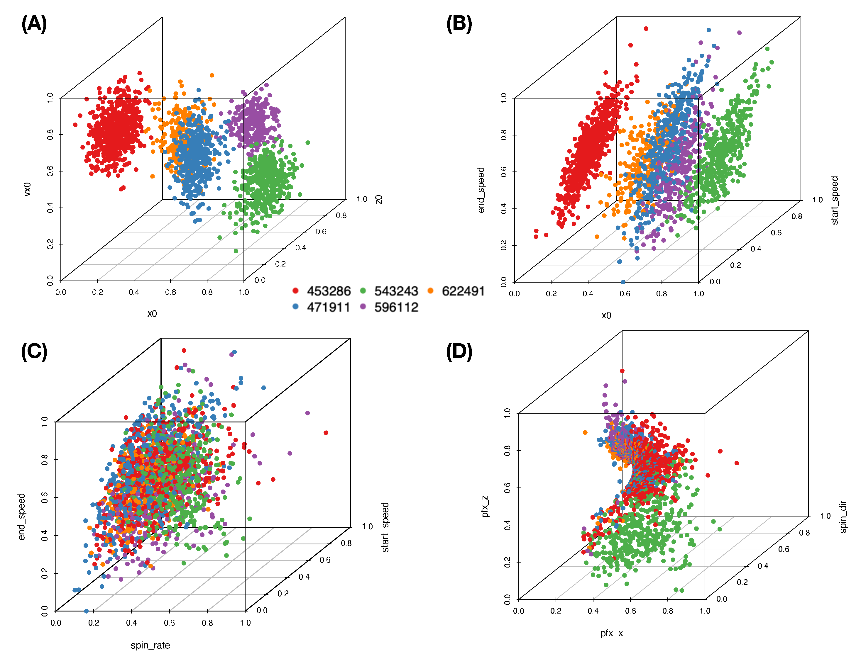
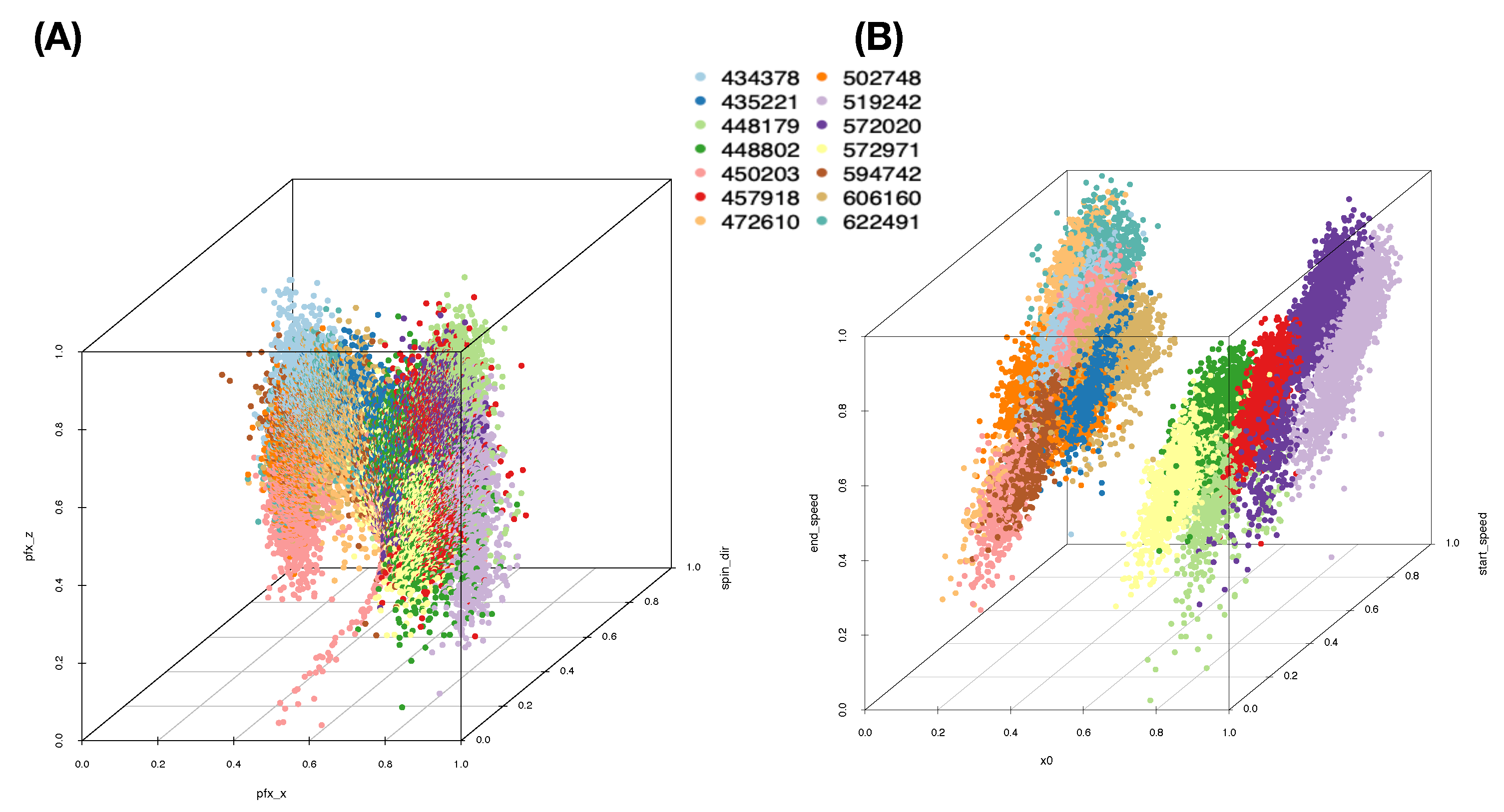
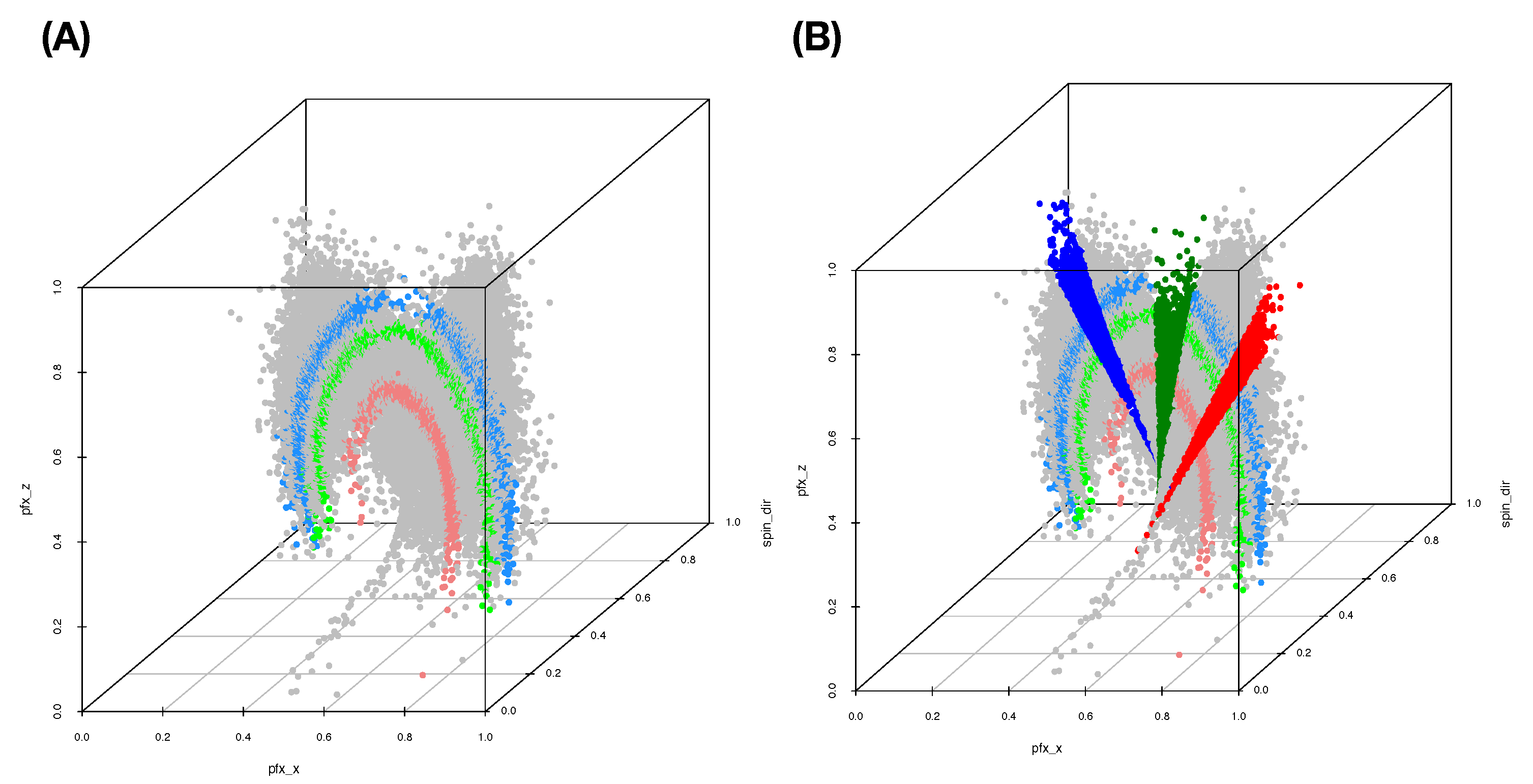
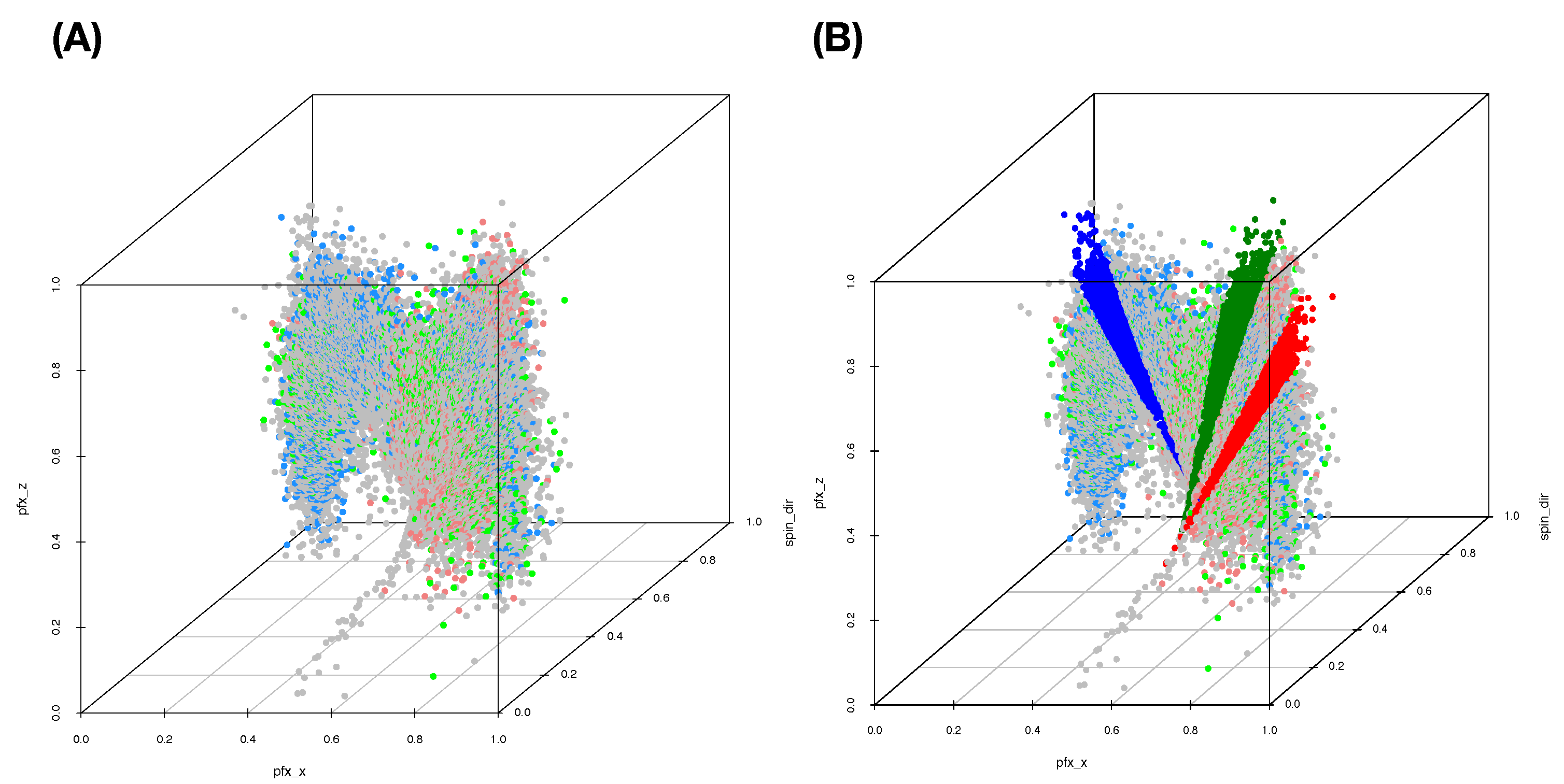
The five computed synergistic feature-groups as five feature-sets give rise to five rather distinct mixing geometries of five pitchers’ point-clouds. Among these five feature-groups, two mixing geometries of two feature-groups are especially revealing in
Figure 5A,B.
We can somehow have a glimpse of the full MCC information content under this MCC setting, mainly through their 3D rotatable plots. To precisely extract and transparently display any mixing geometry with respect to a given feature-set, our computational developments of CEDA for MCC are constructed according to the following three-step protocol.
- [MCC-Q1]
First, based on a given feature-group and its corresponding training data subset, we derive relative closeness among all label-specific point-clouds by performing the first task of CEDA for MCC in the Iris example for all possible label triplets, and then build a feature-group label embedding tree (LET) upon the label space.
- [MCC-Q2]
Second, we devise one universal binary competition of Left-branch-vs.-Right-branch, based
-nearest neighbors (KNN) [
23], for all LET’s internal nodes. We perform the second task of CEDA for MCC in the Iris example for all data points in all labels’ testing data subsets, respectively. Consequently, we build a collection of
L pie charts to represent resultant feature-group specific mixing geometries.
- [MCC-Q3]
Third, we perform the data-driven explorations similar to the third task of CEDA for MCC in the Iris example for a chain of complementary feature-groups. Ideally, we want to discover a chain composed of the first feature-group as a major factor and followed by a short series of feature-groups as minor factors. The results of such a chain are summarized via tabular representations to reveal the collection of mixing geometric pattern-categories of various orders.
Here, as illustrated in the Iris example, a feature-group is an effective candidate for a major factor if the proportion of testing data points falling into mixing geometric categories with “certainty” is indeed as large as possible. Throughout this paper, we use of observed data points for the training data subset and for the testing data subset.
4.2.1. Computing a Label Embedding Tree (Let)
For [MCC-Q1] in our CEDA for MCC protocol, the dimensionality of point-cloud is not an issue. However, it is a key issue for any mathematical definition of a direct distance measure between two point-clouds. For instance, researchers recently have recently applied optimal transport (OT) [
24], Gromov–Hausdorff, or Gromov–Wasstein distances to evaluate a distance between two point-clouds [
25,
26] since such a direct measure is based on the pair’s distribution functions. Not only will the curse of dimensionality apply here, but also their non-robustness to shapes and tails behaviors of distributions will jointly worsen their effectiveness. Thus, such direct distances can be neither practical nor realistic among diverse mixing geometries. To avoid such shortcomings, it is essential to employ the concept of relative-distance or relative-closeness as stated in [MCC-Q1].
In contrast, we demonstrate why results from [MCC-Q1] are inherently robust via the following simple experiment. We randomly select three subsets of data points from three pitchers (as color-coded) with respect to the Feature-Group C, respectively. We construct a heatmap of the distance matrix among all selected 3D data points, as shown in
Figure 8A. It is seen from the heatmap that most partial ordering among all possible triplets of 3D data-points from three pitchers will likely be relatively stable; that is, the (blue, green) label-pair is most likely the smallest among the three pairs. Such inherent stochastic stability of triplet’s partial ordering would result in a robust
dominance matrix among all 10 possible pairs. Consequently, the resultant LET upon the five pitchers, as shown in
Figure 8B, should be very robust.
We interpret through the tree structures of this HC tree as collectively aggregating many pieces of information of partial orderings among these five pitchers (as color-coded), such as
without the need of knowing the ordering between
and
. Here,
denotes the “relative-distance” defined based on a dominance matrix that reflects all possible triplet’s partial orderings, as illustrated in
Figure 6A,B in the Iris example. We formally describe the algorithm for [MCC-Q1] below.
[Algorithm for label embedding tree (LET)]
- [T-1]
Given a set of k features, choose one triple of labels (pitchers) at a time, sample one triple of k-dimensional vectors from the three distinct labels’ training point-clouds, and evaluate three pairwise Euclidean distances. We only record binary partial ordering: which label-pair’s distance is dominated by the two distances of other two label-pairs.
- [T-2]
Repeat Step [T-1] a fixed, but large number of times across many possible triples of labels and summarize and arrange all binary partial orderings of pairwise-distance-dominance into a dominance matrix with all possible label-pairs being arranged along its row and column axes.
- [T-3]
Upon such a dominance matrix, which designates a row-pair dominating a column-pair, each column-sum indicates the relative-closeness of the pair of labels among all possible pairs, while each row-sum indicates the “relative-distance” of the pair of labels.
- [T-4]
The collection of row-sums forms a “relative-distance” matrix of all labels. A label embedding tree (LET) is built based on a HC algorithm on this dominance-based relative-distance matrix.
This algorithm is applicable for all MCC settings with structured data.
4.2.2. Predictive Map of Mixing Geometric Pattern Categories
The tree geometry of LET represents a large-scale component of MCC information content. Based on LET’s binary structures from tree-top to tree-bottom, we explicitly devise a tree-descending series of “Left-branch-vs.-Right-branch” competitions at each internal nodes in this subsection. By letting each of testing data points from all labels going through such a tree-based series of competitions, we can discover the mixing geometry in very fine details. Since the serial results of competitions collectively and precisely bring out entire mixing geometry of all point-clouds (based on training data), this is an efficient way of exposing all geometric mixing patterns involving in all L point-clouds pertaining to k chosen features. Such pattern information is basically invisible when . Even when or 3, such information might be hard to decipher.
For [MCC-Q2] of our CEDA for MCC protocol, we design the following algorithm to expose and extract local mixing geometric information and then summarize all results into a collection of pie charts, called predictive map. This tabular representation reveals MCC information content pertaining to a feature-group in detail.
[Algorithm for the Predictive Map (PM)]
- [P-1]
Take a testing point-vector, say x, from the testing dataset of a label. Starting from the internal-node on the tree top of LET, we perform binary, Left-branch-vs.-Right-branch, competition via —nearest neighbors of x. Here, is used. To decide which branch x belongs, we separate the neighbors with respect to their Left-branch and Right-branch memberships. We declare the winner according to the following policy: (a) one branch dominates in membership count; and (b) if both counts are not significantly different, then we build two membership-specific distance distributions. Upon each distribution, we calculate a pseudo-likelihood (PL) value to the median distance from x to all members of the same branch. We then compare the ratio of the two PL-values with respect to a threshold range : if the PL-ratio falls out of this range with the clear winner being Left-branch or Right-branch, then we go on to the next step; if it falls within the range, we stop the competition process and record no-winner at the internal node.
- [P-2]
Repeat the binary competition of Step [P-1] at the winner branch’s internal node and descend further down along the winning branches until the serial of binary games stops at one no-winner internal node, which can be a branch consisting of one singleton label. Then, we record no-winner internal node’s branch members as the predicted label-set, a singleton, multiple, or none. (The case of empty predicted label-set is a device of zero-shot learning for discovering outlier.)
- [P-3]
Repeat Steps [P-1] and [P-2] for all testing data points across all labels, and then partition each label’s testing set with respect to all its members’ predicted label-sets as categories in a pie chart, as shown in
Figure 9. This feature-group specific collection of pie chart is called predictive map (PM).
On Step-[P-3], instead of using a collection of pie charts, an alternative presentation is to arranging all observed predicted label-sets across all labels along the row axis and involving labels along the column axis, all predictions of testing data points from the testing dataset are summarized into a matrix, which is also called predictive map (PM). This matrix format is employed for presenting results derived from a chain of complementary feature-groups, as shown in the subsection below.
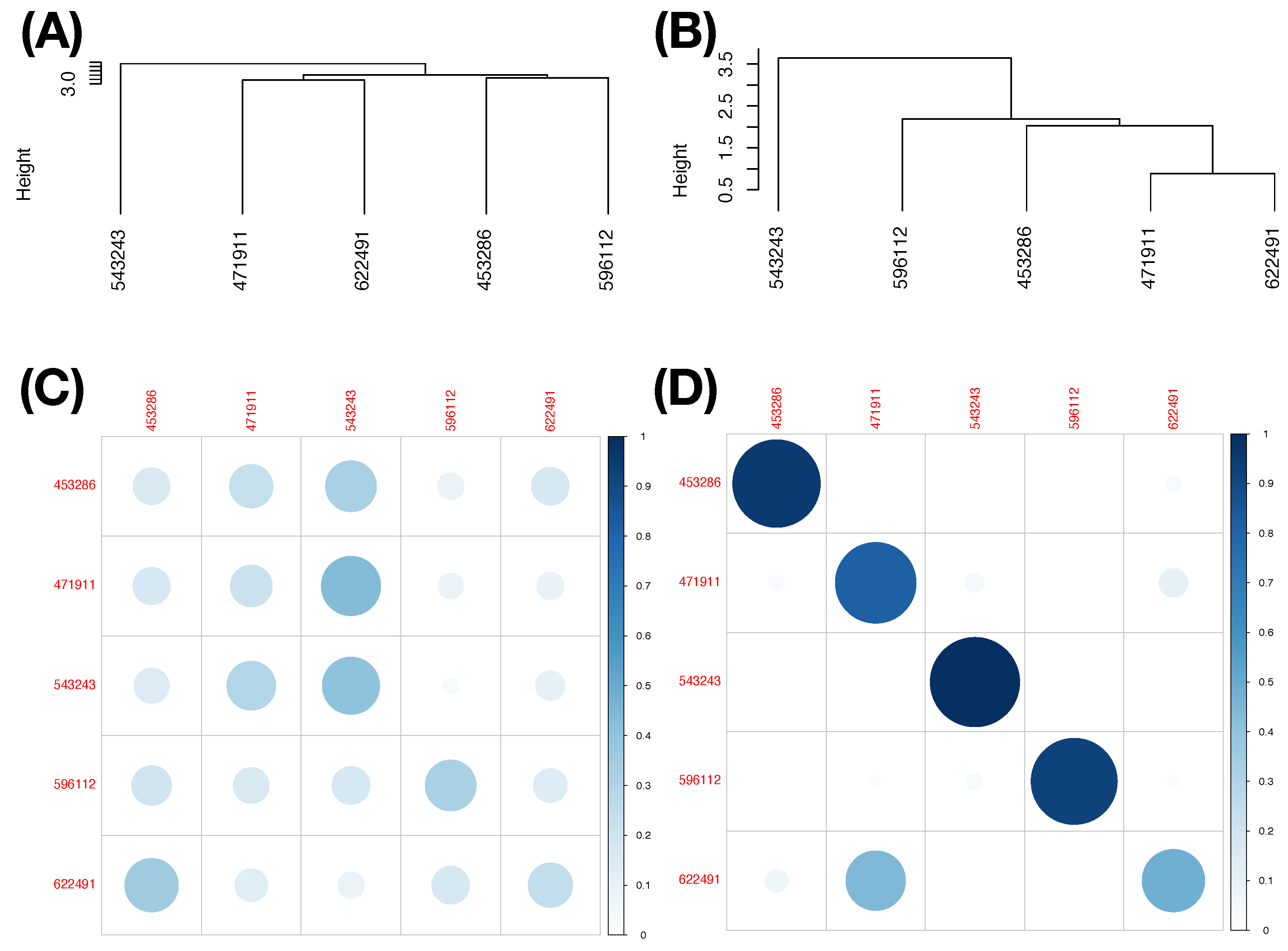
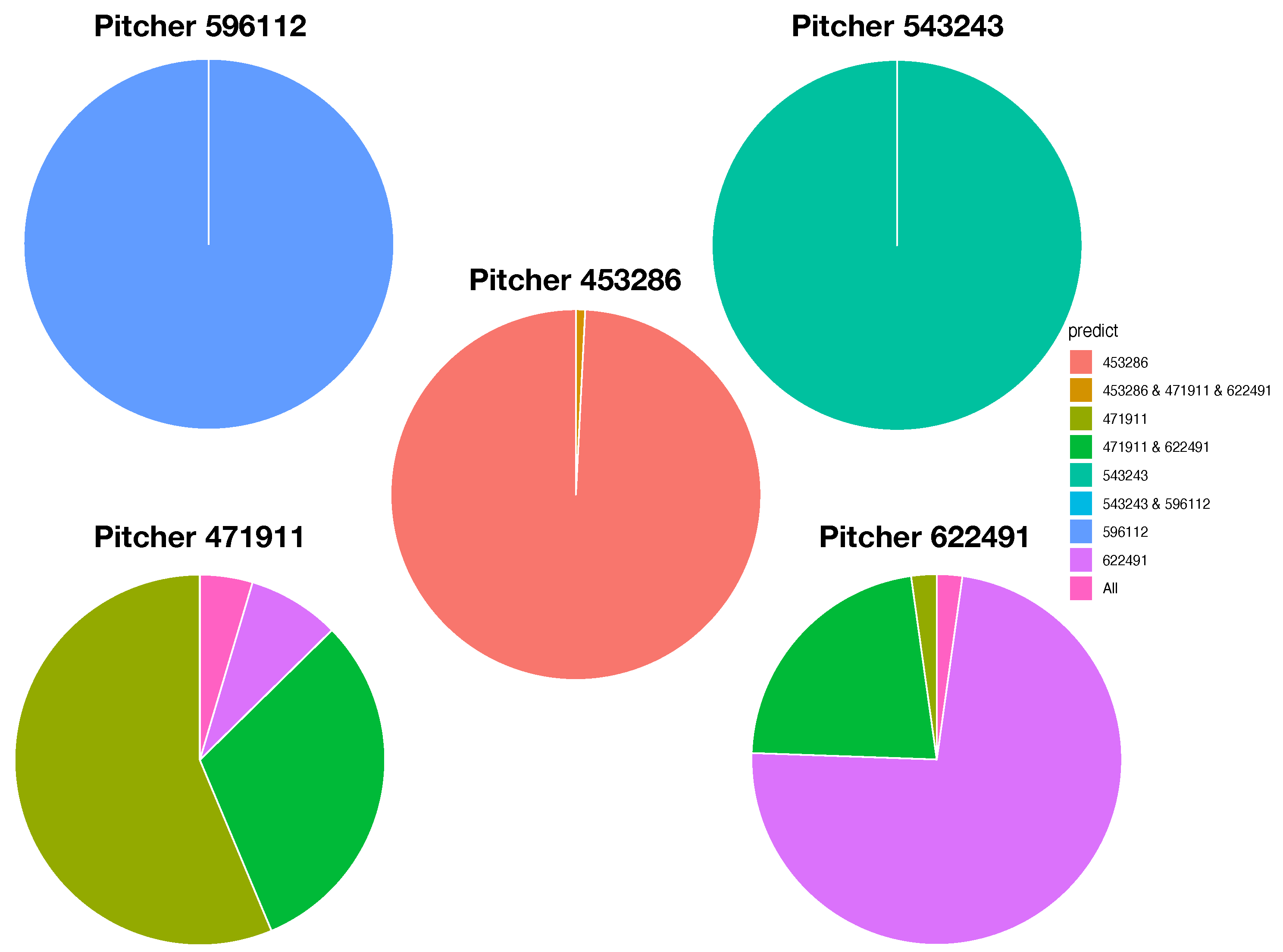
The five pie charts, shown in
Figure 9, reveal very coherent and precise mixing geometric information among the five point-clouds. The two pie charts Pitcher 596112 (purple) and pitcher-543243 (green) indicate that their point-clouds are well separated from the rest of the three point-clouds. It is nearly so for Pitcher 453286 (brown), except a small area of a mixture involving three pitchers: {453286 & 471911 &622491}. It is very significant to note that this mixture of {453286 & 471911 &622491} is uniquely pertaining to Pitcher 453286. No such mixture is found upon any other pitcher. This is a crucial piece of information content based on local scale mixing geometry. Thus, any testing data-point resulted in this pitcher-specific mixture must uniquely belong to Pitcher 453286, not the other two pitchers, Pitcher 471911 and Pitcher 622491. This is what the asymmetry of mixing geometry can offer. From a prediction point of view, we conclude that the pitches of Pitcher 453286 can be perfectly predicted with 100% precision in a singleton format. More examples of such asymmetry are reported below. This mixing geometric asymmetry-based result is at odds with all existing works in statistics and machine learning literature.
Mixing geometric information of Pitcher 471911 and Pitcher 622491 is also diverse and characteristic. More than 50% of pitches of Pitcher 471911 are standing alone and identified as Pitcher 471911, while about 75% of pitches of Pitcher 622491 are standing alone and identified as Pitcher 622491. There are about 20% pitches of Pitcher 471911 and 15% of pitches of Pitcher 622491 being identified for both pitchers, {471911 & 622491}, respectively. It is legitimate to claim that a testing data point falling into this mixture of {471911 & 622491} is predicted as (471911, 622491) because the mixing geometry fully supports such a decision. It is unnecessary or even unnatural to choose one against the other. We need to include extra information computed from different feature-sets in order to separate between these two pitchers.
In both pie charts, there are visible proportions of pitches from both pitchers: Pitcher 471911 and Pitcher 622491 are identified “wrongly”. The reason is that a pitch of Pitcher 472911 is intensively surrounded by pitches of Pitcher 622491 or vice versa. Since this mixing pattern is feature-set specific, such a mixing pattern might be altered significantly with respect to different feature-sets. This is why we need to seek for complementary feature-sets.
In sharp contrast with the above decision-making based on a predictive-map, we explicitly demonstrate why any decision-making scheme producing only singleton-predictors indeed forces us to make mistakes. Consider the choice of threshold range , which is equivalent to using a threshold value 1 on PL-ratio. By employing such a threshold, we force ourselves to choose a winning branch against a losing branch at each internal node LET. Consequentially, all predictive results under such a thresholding scheme are in the form of a singleton. It is essential to note that potential errors are to be accumulated, and, at the same time, the capability of declaring an outlier is discarded. In other words, we force ourselves to make multiple kinds of mistakes by disregarding valuable information that is indeed supported by the training data.
We illustrate results obtained under this thresholding scheme with two less informative feature-sets under Slider’s MCC setting: (1) Feature-Set A; and (2) the feature-set of all features. Their LETs and predictive maps are, respectively, reported in the two columns of
Figure 10: left column (
Figure 10A,C) for the Feature-Set A and right column (
Figure 10B,D) for the feature-set of all features. By arranging each of the two resultant predictive maps into a matrix of proportions with row sum being equal to 1, we see all the potential mistakes across all columns. Although we still can observe the asymmetry of mixing geometries among involving point-clouds, this information is ignored completely. It is seemingly evident that the feature-group of all features is somewhat much more informative than the Feature-Set A. Thus, the potential of making mistake is less. This simple experiment is meant to demonstrate that the choice of feature-group and the asymmetry of mixing geometry are two essential components for computing MCC’s information content.
4.3. Slider’s MCC Information Content
After computing a label embedding tree (LET) and predictive maps (in pie chart format) for any feature-group, the third task of our CEDA for MCC is to discover an effective chain of complementary feature-sets. This chain would lead to visible and explainable MCC’s full information content. Even though we recognize the fact that the great potentials of complementary feature-sets are wide and diverse. Here, we construct a potentially effective chain by choosing a feature-group that can play the role of a major factor under this MCC setting. Since a major factor is supposed to achieve a great degree of certainty across all labels, for further building the chain, we couple this major factor with one or two minor ones.
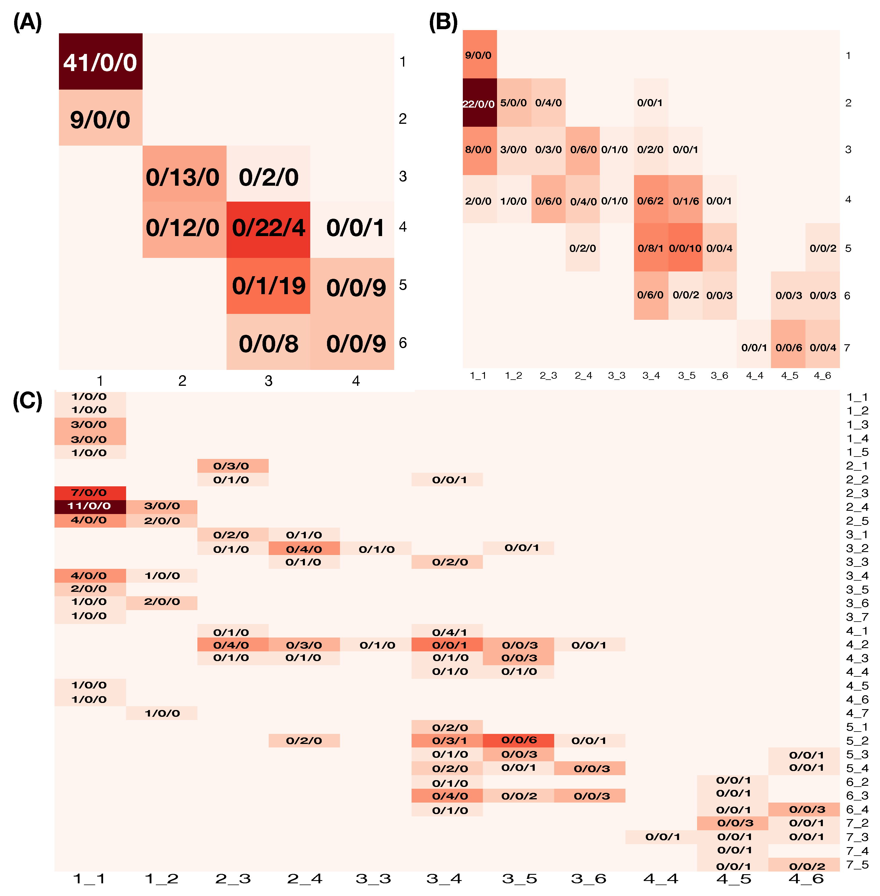
For expositional conciseness, we also encode pitcher-IDs as follows: “a (453286)”, “b (471911)” “c (543243)”, “d (956112)”, and “e (622491)”. Our explorations leads us to the Feature-Group C as the major factor when the choice of threshold range
for PL-ratio is adopted. The five resultant pie charts for the five pitcher-labels, as reported in
Figure 9, bring out the interesting fact: any distinct and unique pitcher-specific local mixing category, not sharing with any other pitchers, certainly identifies the pitcher. Further, its five pie charts are converted into a table, as shown in
Table 1 (left), with respect to eight “observed” mixing geometric pattern-categories arranged and listed on its row axis. In this fashion, MCC information content from Feature-Set C is revealed and organized. The three pitchers {a, c, d} are perfectly separated to their pitcher-specific pattern-categories. The remaining four mixing geometric pattern-categories contain pitches from both Pitcher b and Pitcher e, marked by “*”. Such a pattern-category sharing means a locality of“uncertainty” among involving pitchers. For instance, the category {*b} has 49 pitches from Pitcher b and 1 pitch from Pitcher e, while the category {*e} has 7 pitches from Pitcher b and 33 pitches from Pitcher e.
For [MCC-Q3], we further explore fine-scale MCC information content by exploring potential feature-sets for roles of minor factors. This exploration is performed by dissecting the above localities having uncertainty (under the major factor) as looking through a different perspective via a feature-group. We choose the feature-group {“x0”, “z0”, “spin_dir”} for this minor role. Its pie chart is summarized and presented in
Table 3 (right) with seven categories that are subject to uncertainty. In
Table 4, the four asterisk-marked mixing geometric pattern-categories via Feature-Set C are projected with respect to six mixing geometric pattern-categories (without {a}). From its first three columns for {*b}, we see that the 49 pitches of Pitcher b are exclusively divided into three second-order categories: 34 in {*b-b}, 14 in {*b-be}, and 1 in {all(abcde)}. One pitch from Pitcher e is alone in {*b-e}. Therefore, these 50 pitches are exclusively located. This is a sense of complementary feature-sets.
In contrast, the 40 pitches in category {*e} are divided into two second-order categories: 25 in {*e-e} (with 1 pitch belonging to Pitcher b and 24 belonging to Pitcher e) and 15 in {*e-be} (6 from Pitcher b and 9 from Pitcher e). Therefore, these two second-order categories are subject to uncertainty and need further explorations from another perspective of another feature-group. Likewise, second-order categories are derived from first-order categories {*be} and {*all}. We choose the Feature-Set A–C, including members of three feature-groups A, B, and C as the third feature-group in the chain. Pattern-categories of mixing geometry of Feature-Set A–C are given in
Table 5.
All the third-order mixing geometric pattern-categories are listed in
Table 6. This table shows promising results. There are 15 out of 21 triplet categories obtaining certainty regarding being exclusively in Pitcher b or Pitcher e. This phenomenon manifests clear characters of a chain of third-ordered complementary feature-groups.
As for pitches belonging to the other five categories of third order, geometrically speaking, intensive mixing between Pitcher b and Pitcher e is found within these localities. Therefore, it is reasonable and necessary to make a prediction decision as {Pitcher b, Pitcher e} within these localities. On the other hand, making any singleton-based decision upon such localities is firmly against the evidence supported by the data. Surely, odds-ratios should accompany the predictive label-sets.
In summary, with a carefully selected chain of three complementary feature-groups, the slider dataset’s MCC information content is explored in-depth and collectively represented by its LET and a series of ordered predictive maps. There are at least three notable merits of such MCC information content. The chief one is that the first, second, and third orders of mixing geometric pattern-categories jointly provide the basis for understanding the labeling’s rationales. The second merit is that they offer a platform for error-free decision-making. That is, all predictive results are fully supported by patterns embraced by the data. The third merit is that such serial tabular mixing geometric pattern-categories allow us to dissect the uncertainty of unexplainable black-boxed results derived from popular machine learning algorithms, such as random forest and various boosting approaches. This merit is somehow surprising, as demonstrated after the following subsection, in which we demonstrate the same characters of MCC information content of the curveball dataset.
4.4. Curveball’s MCC Information Content
We report here our CEDA for MCC computational results on the curveball dataset. We employ exactly the same computational algorithms and exploring themes to work out curveball’s MCC information content. The selected chain of complementary feature-groups turns out to be even more efficient in this MCC setting than that of the slider.
The curveball is a pitch-type with top-spin, which is the opposite of a fastball’s back-spin. Unlike fastball, generating top-spin is a bit unnatural. Thus, a curveball pitch in general is much slower than a fastball or slider for any MLB pitcher. Its typical trajectory has a significant vertical drop (measured by “pfx_z”) when reaching the home plate. This drastic drop is caused by the Magnus effect being added onto the gravity force. It is a somewhat effective pitch-type in dealing with batters. In sharp contrast with the slider, its horizontal movement (measured by “pfx_x”) has a narrow range centering around zero.
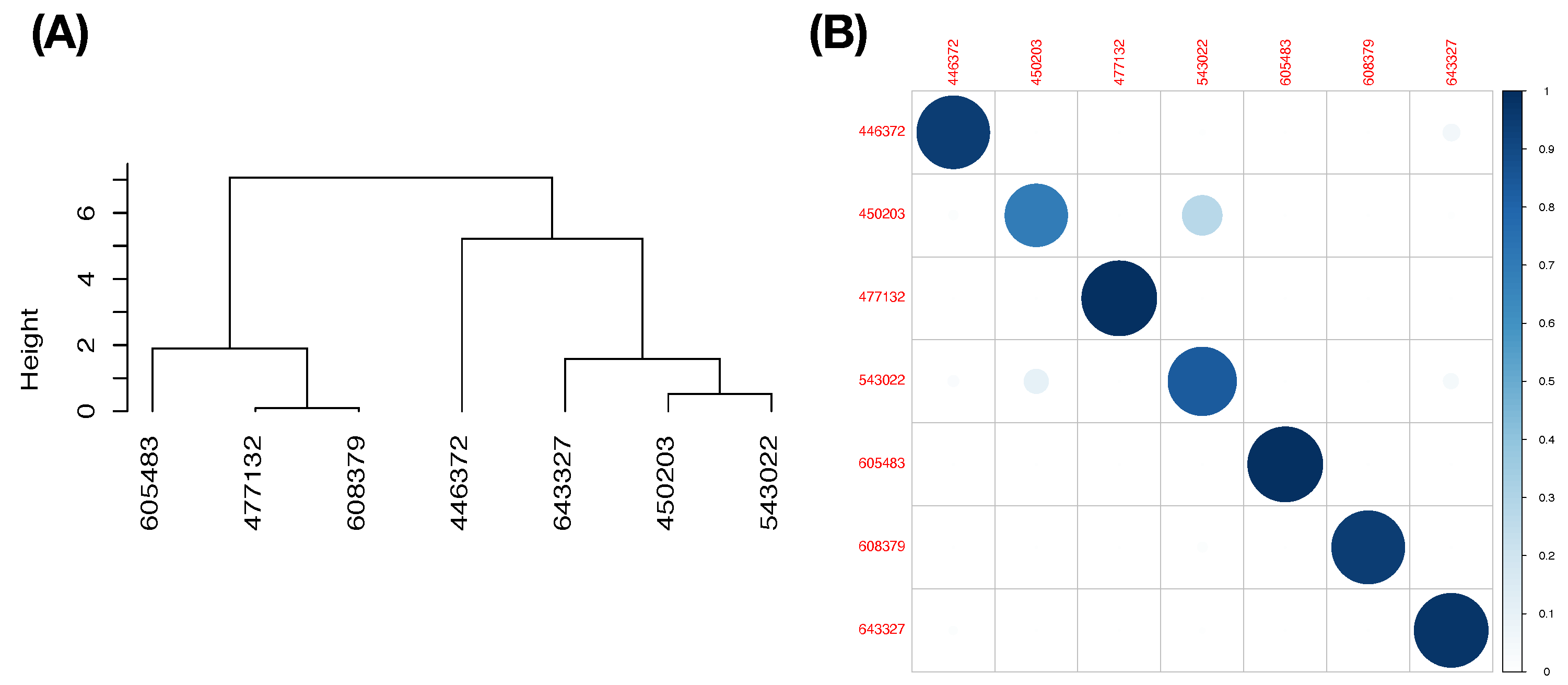
The curveball dataset used here consists of seven
MLB pitchers. We compute its
mutual conditional entropy matrix, as shown in
Figure 4B. Its heatmap reveals six evident blocks as marked along its diagonal. These six highly associated feature-groups are: Group A, {“px”, “x”}; Group B, {“vz0”, “pz”}; Group C, {“spin_dir”, “break_angle”, “ax”, “pfx_x”}; Group D, {“break_length”, “pfx_z”,“az”}. Group E, {“end_speed”, “start_speed”, “vyo”}; and Group F, {“ay”, “spin_rate”, “z0”, “vx0”, “x0”}. We also calculate the directed associations of the 19 features toward the label space and rank them. The six highest associations (in increasing order) are: {“x0”, “z0”, “spin_dir”, “start_speed”, “vy0”, “break_angle”}. This feature-set of six is denoted as BB.
With the same 4-to-1 ratio for training-to-testing data subsets, our CEDA follows the same CEDA for MCC protocol as we previously have done under slider’s MCC setting. Our choice of a chain of complementary feature-groups begins with a feature-group, denoted as DEF, including members from three feature-groups: D–F (
Figure 4B). As the major factor of the chain, the LET of feature-set DEF and its predictive map with the thresholding scheme with
are given in
Figure 11A,B, respectively. Once again, such a predictive map shows asymmetry of mixing geometries and the amounts of errors by forcefully committing to a singleton label-predictor.
In contrast, with respect to feature-group DEF and the choice of threshold range
for PL-ratio, the resultant predictive map is reported in
Table 7. This feature-set DEF seems rather efficient. We see that, except Pitcher b (with ID: 450203), the other six pitchers are nearly exclusively predicted. Pitcher-IDs are encoded as following: Pitcher a (446372), Pitcher c (477132), Pitcher d (543022), Pitcher e (605483), Pitcher f (608379), and Pitcher g (643327). Among the 12 mixing geometric pattern-categories of the first order, six are pitcher-ID specific, while six ategories have uncertainty. Next, we choose the feature-group BB to be the second feature-group as a minor factor in the chain to further explore the fine-scale MCC information content.
With the chain of two feature-groups, DEF to BB, such chain results are reported in
Table 8. The majority of the second-order mixing geometric pattern-categories turn out to be pitcher specific, while those with uncertainty have relatively extreme odds-ratios. We indeed can explore further. We stop here to avoid repeating similar messages regarding the effectiveness of such chains of complementary feature-groups. The above two tables of local mixing geometric pattern-categories demonstrate the effects of two complementary feature-sets, and at the same time jointly reveal the curveball’s MCC information content. Such a chain of two feature-groups offers perfect predictive decision-making with explainable supporting evidence. Likewise, the platform consisting of the first and second orders of mixing geometric pattern-categories can map out machine learning methodologies’ uncertainly, as discussed below.
4.5. Dissecting Uncertainty of Results from Machine Learning Algorithm
Under MCC settings, ML algorithms, such as random forest [
27] and various boosting approaches [
28,
29], are popularly employed. They can achieve low classification error rates. Such successes are mainly seen when the number of features
K is large relative to the size of label space
L. Many factors certainly have contributed significantly to such successes. However, all these decisions are derived from black-boxes in the sense of no reasons and interpretations attached. This issue of non-interpretability is a serious one from the perspectives of real-world applications as well as sciences, since, even if they can potentially achieve very low error rates, these error rates are not equal to zeros. That is, all these machine learning results under any MCC setting are subject to the uncertainty of being simultaneously right and wrong.
Indeed, our MCC information content can serve as an ultimate standard of validity for uncertainty resulting from machine learning algorithms. The validity check is subject to each testing data point to both CEDA and any machine learning algorithm. Then, we view and check which one of the mixing geometric pattern-categories a testing data point’s ML decision falls into. Such a check leads to one of the following four possibilities, with a ML decision landing in the mixing geometric pattern-category:
- 1. [certainty–coherent]:
with certainty, and they are coherent;
- 2. [certainty–incoherent]:
with certainty, but they are incoherent;
- 3. [uncertainty–coherent]:
with uncertainty and they are coherent; and
- 4. [uncertainty–incoherent]:
with uncertainty, but they are incoherent.
The certainty–coherent case serves as a confirmation of the ML-decision. Both cases of certainty–incoherent and uncertainty–incoherent likely point out that the ML’ predictive result is“definitely” wrong. There exists still uncertainty when a ML predictive result falls into uncertainty–coherent case. However, it will be 100% correct if we report our predictive decision based on the mixing geometric pattern-category. Upon these four cases, it seems that all ML methodologies can evidently be significantly strengthened by projecting their predictive results onto our MCC information content. At the same time, we resolve the interpretation issue completely.
We illustrate such conclusions through applying random forest on the slider and curveball datasets. Our experiments applied random forest multiple times and two versions of boosting multiple times. All results are relatively consistent with the above conclusions. Thus, we only report results from the random forest.
In
Table 9, we see that random forest (RF) makes 13 errors: 2 from Pitcher b being assigned to Pitcher e, 1 from Pitcher c being assigned to Pitcher b, and 10 from Pitcher e being assigned to Pitcher b. For the first-order mixing geometric pattern-categories, the certainty–incoherent error of Pitcher b prediction on one pitch of Pitcher c has been confirmed at the Category c. Among 12 remaining errors going into the second-order mixing geometric pattern-categories in
Table 4, we see that one RF’s error is confirmed in the Category b–e in
Table 10. The 11 remaining errors going into the third order mixing geometric pattern-categories in
Table 6, we see two pitches of Pitcher e are confirmed in e–e–be and e–e–abe; the other nine pitches are in [uncertainty–coherent] case: two from Pitcher b and seven from Pitcher e, are all in mixing geometric pattern-categories with uncertainty.
Such a dissection on the uncertainty of Random Forest’s errors brings out the fact that all its errors are likely coming from rather intensive mixing localities of the geometry of all involving point-clouds. From this perspective, it would be advantageous to make ML predictions with projections into mixing geometric pattern-categories of MCC information content. This conclusion is proper throughout all experiments via two versions of boosting as well.
To iterate such a conclusive statement, we again view the errors made by random forest on the curveball dataset from the perspective of its MCC information content. There are 14 errors committed by random forest on one application, as shown in
Table 11. In
Table 12, all 14 errors fall into first-order mixing geometric pattern-categories with uncertainty, as shown in
Table 7. Further, in
Table 12 and due to one (d–bd) and one (bdg–db) being corrected, 12 out of 14 fall into the second-order mixing geometric pattern-categories, as shown in
Table 8. Likewise, most errors from the two versions of boosting approaches are also found in an MCC’s mixing geometric pattern-category with uncertainty. Again, we reiterate that it would be advantageous to make ML predictions coupled with projections into mixing geometric pattern-categories of MCC information content.


