
Normalized Sombor Indices as Complexity Measures of Random Networks

 ,
,  and
and 
Abstract
:1. Introduction
2. Computational Properties of Sombor Indices on Random Networks
2.1. Sombor Indices on Erdös-Rényi Networks
- (i)
- (ii)
- (iii)
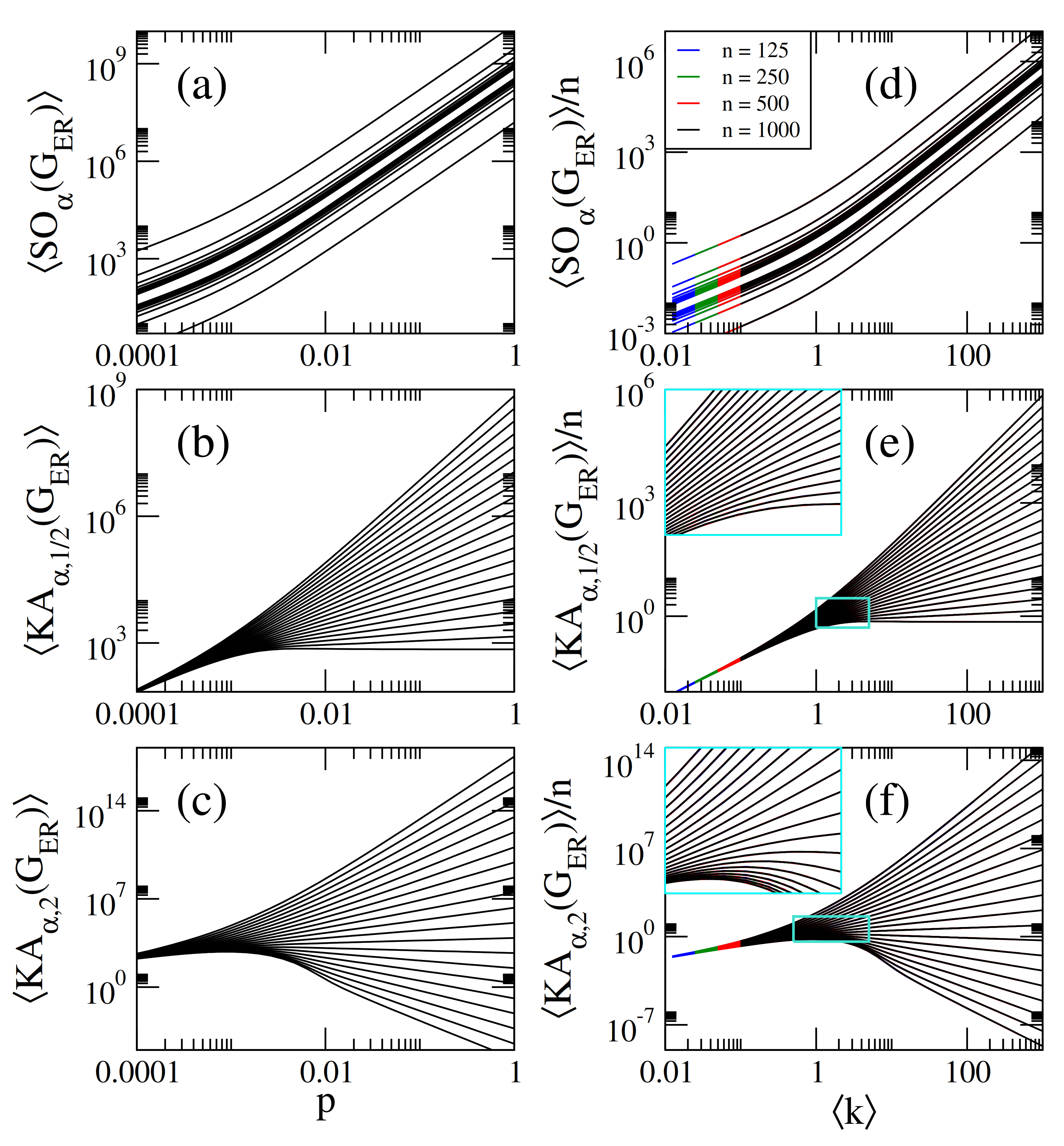
- The curves of show three different behaviors as a function of p depending on the values of and : For , they grow for small p, approach a maximum value and then decrease when p is further increased. For , they are monotonically increasing functions of p. For the curves saturate above a given value of p. For and , the cases reported in Figure 2c,d, we found and , respectively.
- (iv)
- Therefore, for , the average values of the Sombor indices are well approximated by:In Figure 1a–c, we show that Equations (7)–(9) (dashed lines) indeed describe well the data (thick full curves) for large enough p. We also verified that Equations (10) and (11) describe well the data for reported in Figure 2a–c, however we did not include them to avoid figure saturation.
2.2. Sombor Indices on Random Geometric Graphs
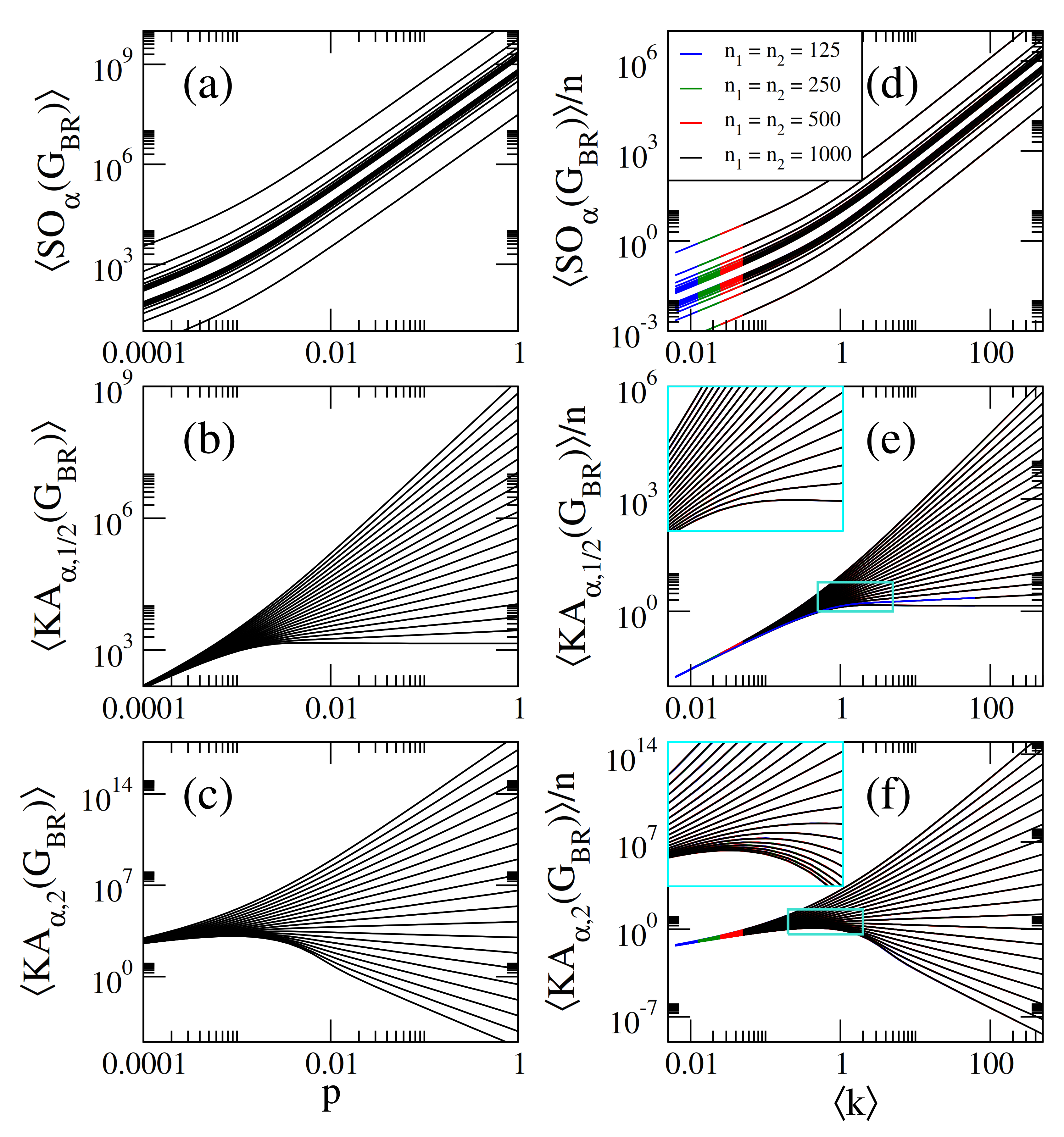
2.3. Sombor Indices on Bipartite Random Networks
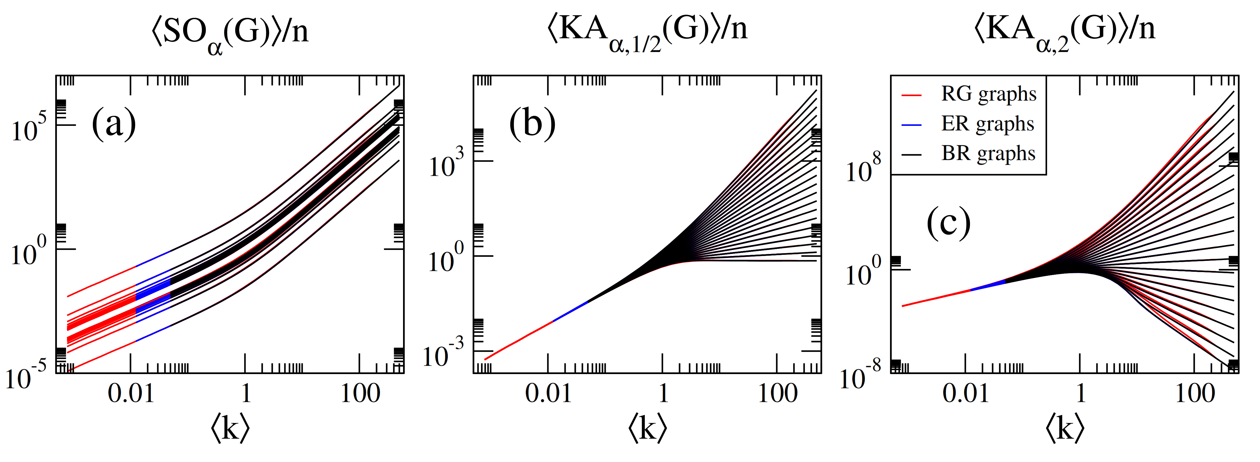
3. General Scaling of Sombor Indices on Random Networks
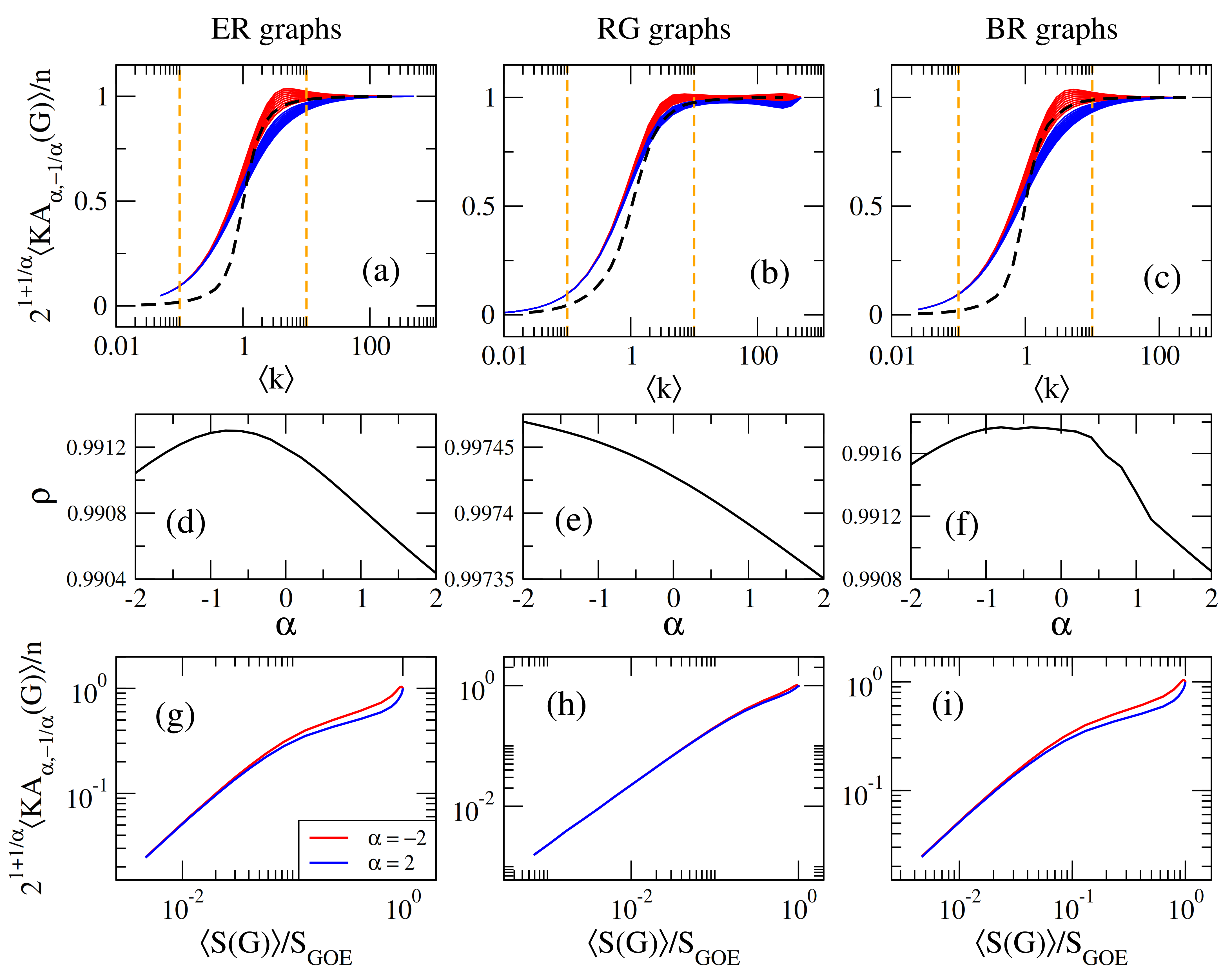
4. Sombor Indices as Complexity Mesures for Random Networks
Correlation between the Average Index and the Average Shannon Entropy
5. Conclusions
Author Contributions
Funding
Data Availability Statement
Conflicts of Interest
References
- Gutman, I. Geometric approach to degree-based topological indices: Sombor indices. MATCH Commun. Math. Comput. Chem. 2021, 86, 11–16. [Google Scholar]
- Kulli, V.R.; Gutman, I. Computation of Sombor indices of certain networks. SSRG Int. J. Appl. Chem. 2021, 8, 1–5. [Google Scholar]
- Lina, Z.; Zhoub, T.; Kullic, V.R.; Miao, L. On the first Banhatti-Sombor index. arXiv 2021, arXiv:2104.03615. [Google Scholar]
- Reti, T.; Doslic, T.; Ali, A. On the Sombor index of graphs. Contrib. Math. 2021, 3, 11–18. [Google Scholar]
- Kulli, V.R. The (a,b)-KA indices of polycyclic aromatic hydrocarbons and benzenoid systems. Int. J. Math. Trends Technol. 2019, 65, 115–120. [Google Scholar]
- Zhou, B.; Trinajstić, N. On general sum-connectivity index. J. Math. Chem. 2010, 47, 210–218. [Google Scholar] [CrossRef]
- Kulli, V.R. δ-Sombor index and its exponential for certain nanotubes. Ann. Pure Appl. Math. 2021, 23, 37–42. [Google Scholar]
- Cruz, R.; Gutman, I.; Rada, J. Sombor index of chemical graphs. Appl. Math. Comput. 2021, 399, 126018. [Google Scholar]
- Cruz, R.; Rada, J. Extremal values of the Sombor index in unicyclic and bicyclic graphs. J. Math. Chem. 2021, 59, 1098–1116. [Google Scholar] [CrossRef]
- Ghanbari, N.; Alikhani, S. Sombor index of certain graphs. arXiv 2021, arXiv:2102.10409. [Google Scholar]
- Alikhani, S.; Ghanbari, N. Sombor index of polymers. MATCH Commun. Math. Comput. Chem. 2021, 86, 715–728. [Google Scholar]
- Fang, X.; You, L.; Liu, H. The expected values of Sombor indices in random hexagonal chains, phenylene chains and Sombor indices of some chemical graphs. Int. J. Quantum Chem. 2021. [Google Scholar] [CrossRef]
- Deng, H.; Tang, Z.; Wu, R. Molecular trees with extremal values of Sombor indices. Quantum Chem. 2021, 121, e26622. [Google Scholar] [CrossRef]
- Liu, H. Ordering chemical graphs by their Sombor indices. arXiv 2021, arXiv:2103.05995. [Google Scholar]
- Liu, H. Maximum Sombor index among cacti. arXiv 2021, arXiv:2103.07924. [Google Scholar]
- Liu, H.; You, L.; Huang, Y. Ordering chemical graphs by Sombor indices and its applications. MATCH Commun. Math. Comput. Chem. 2021, 87, 2022. [Google Scholar]
- Zhou, T.; Lin, Z.; Miao, L. The Sombor index of trees and unicyclic graphs with given matching number. arXiv 2021, arXiv:2103.04645. [Google Scholar]
- Zhou, T.; Lin, Z.; Miao, L. The Sombor index of trees and unicyclic graphs with given maximum degree. arXiv 2021, arXiv:2103.07947. [Google Scholar]
- Gutman, I. Some basic properties of Sombor indices. Open J. Discret. Appl. Math. 2021, 4, 1–3. [Google Scholar] [CrossRef]
- Milovanovic, I.; Milovanovic, E.; Mateji, M. On some mathematical properties of Sombor indices. Bull. Int. Math. Virtual Inst. 2021, 11, 341–353. [Google Scholar]
- Das, K.C.; Cevik, A.S.; Cangul, I.N.; Shang, Y. On Sombor index. Symmetry 2021, 13, 140. [Google Scholar] [CrossRef]
- Rada, J.; Rodriguez, J.M.; Sigarreta, J.M. General properties on Sombor indices. Discret. Appl. Math. 2021, 299, 87–97. [Google Scholar] [CrossRef]
- Milovanović, I.; Milovanović, E.; Ali, A.; Matejić, M. Some results on the Sombor indices of graphs. Contrib. Math. 2021, 3, 5–67. [Google Scholar]
- Wang, Z.; Mao, Y.; Li, Y.; Furtula, B. On relations between Sombor and other degree-based indices. J. Appl. Math. Comput. 2021. [Google Scholar] [CrossRef]
- Redzepovic, I. Chemical applicability of Sombor indices. J. Serb. Chem Soc. 2021, 86, 445–457. [Google Scholar] [CrossRef]
- Lin, Z. On the spectral radius, energy and Estrada index of the Sombor matrix of graphs. arXiv 2021, arXiv:2102.03960. [Google Scholar]
- Solomonoff, R.; Rapoport, A. Connectivity of random nets. Bull. Math. Biophys. 1951, 13, 107–117. [Google Scholar] [CrossRef]
- Erdös, P.; Rényi, A. On random graphs. Publ. Math. Debr. Hung. 1959, 6, 290–297. [Google Scholar]
- Erdös, P.; Rényi, A. On the evolution of random graphs. Inst. Hung. Acad. Sci. 1960, 5, 17–61. [Google Scholar]
- Erdös, P.; Rényi, A. On the strength of connectedness of a random graph. Acta Math. Hung. 1961, 12, 261–267. [Google Scholar] [CrossRef]
- Dall, J.; Christensen, M. Random geometric graphs. Phys. Rev. E 2002, 66, 016121. [Google Scholar] [CrossRef] [Green Version]
- Penrose, M. Random Geometric Graphs; Oxford University Press: Oxford, UK, 2003. [Google Scholar]
- Martínez-Martínez, C.T.; Mendez-Bermudez, J.A.; Rodríguez, J.M.; Sigarreta, J.M. Computational and analytical studies of the Randić index in Erdös–Rényi models. Appl. Math. Comput. 2020, 377, 125137. [Google Scholar] [CrossRef] [Green Version]
- Martínez-Martínez, C.T.; Mendez-Bermudez, J.A.; Rodríguez, J.M.; Sigarreta, J.M. Computational and analytical studies of the harmonic index in Erdös–Rényi models. MATCH Commun. Math. Comput. Chem. 2021, 85, 395–426. [Google Scholar]
- Estrada, E.; Sheerin, M. Random rectangular graphs. Phys. Rev. E 2015, 91, 042805. [Google Scholar] [CrossRef] [Green Version]
- Mendez-Bermudez, J.A.; Alcazar-Lopez, A.; Martinez-Mendoza, A.J.; Rodrigues, F.A.; Peron, T.K.D. Universality in the spectral and eigenfunction properties of random networks. Phys. Rev. E 2015, 91, 032122. [Google Scholar] [CrossRef] [PubMed] [Green Version]
- Alonso, L.; Mendez-Bermudez, J.A.; Gonzalez-Melendrez, A.; Moreno, Y. Weighted random-geometric and random-rectangular graphs: Spectral and eigenfunction properties of the adjacency matrix. J. Complex Netw. 2018, 6, 753. [Google Scholar] [CrossRef]
- Aguilar-Sanchez, R.; Mendez-Bermudez, J.A.; Rodrigues, F.A.; Sigarreta-Almira, J.M. Topological versus spectral properties of random geometric graphs. Phys. Rev. E 2020, 102, 042306. [Google Scholar] [CrossRef] [PubMed]
- Metha, M.L. Random Matrices; Elsevier: Amsterdam, The Netherlands, 2004. [Google Scholar]
- Haake, F. Quantum Signatures of Chaos; Springer: Berlin/Heidelberg, Germany, 2010. [Google Scholar]
- Torres-Vargas, G.; Fossion, R.; Mendez-Bermudez, J.A. Normal mode analysis of spectra of random networks. Phys. A 2020, 545, 123298. [Google Scholar] [CrossRef] [Green Version]


Publisher’s Note: MDPI stays neutral with regard to jurisdictional claims in published maps and institutional affiliations. |
© 2021 by the authors. Licensee MDPI, Basel, Switzerland. This article is an open access article distributed under the terms and conditions of the Creative Commons Attribution (CC BY) license (https://creativecommons.org/licenses/by/4.0/).
Share and Cite
Aguilar-Sánchez, R.; Méndez-Bermúdez, J.A.; Rodríguez, J.M.; Sigarreta, J.M. Normalized Sombor Indices as Complexity Measures of Random Networks. Entropy 2021, 23, 976. https://doi.org/10.3390/e23080976
Aguilar-Sánchez R, Méndez-Bermúdez JA, Rodríguez JM, Sigarreta JM. Normalized Sombor Indices as Complexity Measures of Random Networks. Entropy. 2021; 23(8):976. https://doi.org/10.3390/e23080976
Chicago/Turabian StyleAguilar-Sánchez, R., J. A. Méndez-Bermúdez, José M. Rodríguez, and José M. Sigarreta. 2021. "Normalized Sombor Indices as Complexity Measures of Random Networks" Entropy 23, no. 8: 976. https://doi.org/10.3390/e23080976
APA StyleAguilar-Sánchez, R., Méndez-Bermúdez, J. A., Rodríguez, J. M., & Sigarreta, J. M. (2021). Normalized Sombor Indices as Complexity Measures of Random Networks. Entropy, 23(8), 976. https://doi.org/10.3390/e23080976