1. Introduction
The majority of scientific fields, such as biology [
1], neuroscience [
2], medicine, sociology and psychology [
3] and many others [
4], involve dynamics of complex systems [
5,
6]. Scientists and experts in such fields typically can only imagine or even briefly outline various potential response-vs.-covariate (Re-Co) relationships in an attempt to characterize the dynamics of their complex systems of interest [
7]. Given that no explicit functional form of such Re-Co relationships is available, such scientists still go ahead and collect structured data sets by investing great efforts in choosing which features for the role of response variable, and which features for the role of covariate variables. Such choices of features are indeed critical for the sciences because their successes rely entirely on whether such structured data sets can embrace the essence of the targeted Re-Co dynamics or not.
After scientists achieve their scientific quests by generating structured data sets upon the complex systems of interest, it becomes not only very natural, but also very important to ask the following specific question: When such structured data sets are in the data analysts’ hands, what is the most essential common goal of data analysis? This goal is certainly not aimed at an explicit system of equations, nor at a complete set of functional descriptions of the targeted Re-Co dynamic. Instead, this goal can and shall be oriented to decode the scientists’ authentic knowledge and intelligence about the complex systems of interest, and one step further to go beyond the current state of understanding.
In sharp contrast, nearly all statistical model-based data analyses on any structured data sets pertaining to wide-range of Re-Co dynamics always assume an explicit functional structure linking the response variables to covariate variables, including hypothesis testing [
8], analysis of variance (ANOVA) and the many variants of regression analysis [
9,
10], including generalized linear models and log-linear models [
11,
12]. By framing rather complex Re-Co dynamics with rather simplistic explicit functional structures, statistical model-based data analysis surely will run the dangers of hijacking data’s authentic information content. With such dangers in mind, it is natural to ask the reverse question: What if we can reformulate all fundamental statistical tasks to fit under a framework of response-vs.-covariate (Re-Co) dynamics without explicit functional forms and extract data’s authentic information content of data sets?
As the theme of this paper, we demonstrate a positive answer to the above fundamental question. The chief merits of such demonstrations are that we not only can do nearly all data analysis without statistical modeling, but more importantly we can reveal data’s authentic information content to foster true understanding about the complex systems of interest. Our computational developments are illustrated through a series of 6 well-known statistical topic issues with increasing complexity. All successfully revealed information content is visible and interpretable.
The positive answer resides in the paradigm called Categorical Exploratory Data Analysis (CEDA) with its heart anchored at a major factor selection protocol, which has been under developing in a series of published works [
13,
14,
15,
16] and a recently completed work [
17]. For demonstrating the positive answer, this paper establishes practical guidelines for evaluating Theoretical Information Measurements, in particular Shannon’s conditional entropy (CE) and mutual information between the response variables and covariate variables, denoted as
[
18], which are the basis of CEDA and major factor selection protocol.
Along the process of establishing such computational guidelines, we characterize four theme-components in CEDA and the major factor selection protocol:
- TC-1.
Our practical guidelines are established here for evaluating CE and without requiring consistent estimations of their theoretical population-version of measurements.
- TC-2.
All entropy-related evaluations are carried out on a contingency table platform, so learned practical guidelines also provide ways of relieving from the effects of the curse of dimensionality and ascertaining for [C1:confirmable] criterion, which is a kind of relative-reliability.
- TC-3.
CEDA is free of man-made assumption and structures, so consequently its inferences are carried out with natural reliability.
- TC-4.
CEDA only employs data’s categorical nature, so the confirmed collection of major factors indeed reveals data’s authentic information content disregarding data types.
The theme-component [TC-1] allows us to avoid many technical and difficult issues encountered in estimating the theoretical information measurement [
19,
20]. [TC-1] and [TC-2] together make CEDA’s major factor selection protocol very distinct to model-based feature selection based on mutual information evaluations [
21,
22,
23,
24], while [TC-3] makes CEDA’s inferences realistic, and [TC-4] makes CEDA to provide authentic information content with very wide applicability.
For specifically illustrating these four theme-components, we consider a structured data set consisting of data points that are measured and collected in a D vector format with respect to features. The first L components are the designated response (Re) features’ measurements or categories, denoted as , and the rest of K components are K covariate (Co) features’ measurements or categories, denoted as . It is essential to note that some or even all covariate features could be categorical. Thus, data analysts’ task is prescribed as precisely extracting the authentic associative relations between and based on a structured data set.
By extracting authentic associations between response and covariate features, various Theoretical Information Measurements are employed under the structured data setting in [
13,
14,
15,
16,
17]. In particular, Re-Co directional associations developed in CEDA and its major factor selection protocol rely on evaluations of Shannon conditional entropy (CE) and mutual information (
) that are all carried out upon the contingency table platform. This platform is indeed very flexible and adaptable to the number of features on row- and column-axes as well as the total size of data points. Such a key characteristic makes CEDA very versatile in applicability. We explain in more detail as follows.
On the response side, a collection of categories of response features (pertaining to
) is determined with respect to their categorical nature and sample size. Likewise, on the covariate side, a collection of categories for each 1D covariate feature (pertaining to
for
) is chosen accordingly. It is noted that a continuous feature is categorized with respect to its histogram [
25]. If
, then the entire collection of response categories will consist of all non-empty cells or hypercubes of
LD contingency tables. However, when
L is large, the total number of
LD hypercubes could be too large for a finite data set in the sense that many hypercubes are occupied by very few data points. This is known as the effect of the curse of dimensionality. To avoid such an effect, clustering algorithms, such as Hierarchical clustering or K-means algorithms, can also be performed for fusing the
L response features (upon their original continuous measurement scales or their contingency tables when involving categorical ones) into one single categorical response variable. The number of categories can be pre-determined for K-means algorithm or determined by cutting a Hierarchical clustering tree in a fashion such as there is only one tree branch per category. The essential idea behind such feature-fusing operations is to retain the structural dependency among these
L response features, while at the same time reducing the detrimental effect of the curse of dimensionality.
In contrast, singleton and joint (or interacting) effects of all possible subsets of are theoretically potential on the covariate side. However, it is practically known that any high order interacting effects needed to be considered are to a great extent determined by the sample size. That is, a covariate-vs.-response contingency table platform can vary greatly in dimensions: large or small. When viewing a contingency table as a high-dimensional histogram, which is a naive form of density estimation, the curse of dimensionality, or so-called finite sample phenomenon, is supposed to affect our conditional entropy evaluations whenever this table’s dimension is large relative to data’s sample size. We use the notation (rows-vs.-columns) for a contingency table of a covariate variable subset and response variable . As a convention, the categories of are arranged along its column-axis, while the categories of A are arranged along the row-axis. This row-axis would expand with respect to memberships of A.
In CEDA, the associative patterns between any
and
would be discovered and evaluated ucing the contingency table
. It is necessary to reiterate that
can be viewed as a “joint histogram” or “density estimation” of all features contained in
A and
. From this perspective, when the dimension of
increasingly expands as
A including more variables, it is expected that its dimensionality would affect the comparability and reliability of conditional entropy evaluations. Consequently, for comparability purposes, this criterion [C1:confirmable] in CEDA arises. This criterion is based on a so-called data mimicking operation developed in [
14], as will be described in the following paragraphs.
Let
denote one mimicry of
A in the ideal sense of having the same deterministic and stochastic structures. In other words,
is generated to have the same empirical categorical distribution of
A, see [
14] for construction details. More practically speaking, if the empirical categorical distribution of
A is represented by a contingency table, then, given the observed vector of row-sums,
would be another contingency table that has the same lattice dimension and all its row-vectors are generated from Multinomial distribution with parameters specified by the corresponding row-sum and the corresponding vector of observed proportions in
A’s contingency table. It is noted that
is constructed independent of
, that is,
is stochastically independent of
[
14].
Denote the mutual information of of A be based on , and likewise based on . The [C1:confirmable] used in CEDA is referred to as the degree of certainty that is far beyond the upper limit of confidence region based on the empirical distribution of . This [C1:confirmable] criterion is indeed in accordance with CEDA’s theme components: [TC-2] and [TC-3], regarding the merits of a contingency table platform in dealing with the curse of dimensionality and facilitating reliability. It is critical to note that we are not estimating the theoretical mutual information of and A here, and we just want to computationally make sure that is significantly above zero with great reliability under the reality of having only a finite amount of data points at hand.
Henceforth, it is a critical fact in all applications of CEDA: a covariate feature set is confirmed as having effects on
only when the [C1: confirmable] criterion of
is established. This concept makes possible for [TC-1] by doing without the nonparametric estimations of Shannon entropy for a continuous distribution function as well as the mutual information for two sets of continuous variables, which have been the long standing problems in physics and neural computing (see theoretical details in [
19] and computational protocols based on biGamma function in [
20]).
Here, we do not take the view of contingency table as a setup of Grenander’s Method of Sieves (MoS) [
26] in this paper. Though MoS can be a choice for practical reasons and computing issues involving many dimensional features or variables, we do not concern primarily on estimating the population-versions of CEs and
per se, nor the induced sieves biases. Rather, the dimensions of contingency tables are made adaptable to the necessity of accommodating multiple covariate feature-members in
A. Within such cases, the collection of categories of
A might be built based on hierarchical or K-means clustering algorithms. From this perspective, computations for theoretical conditional entropy and mutual information between multiple dimensional covariate and possibly multi-dimensional
Y are neither realistically nor practically possible, due to the limited size of the available data sets. Since this kind of sieves is data dependent, the computations for sieve biases can be much more complicate than that covered in [
19].
In this paper, we illustrate and carry out CEDA coupled with its major factor selection protocol through a series of 6 classic statistical topic examples, within each of which various scenarios are also considered. By building contingency tables across various dimensions with respect to different sample sizes, we attempt to reveal the robustness of CEDA resolutions to statistical topic issues. On one hand, we learn practical guidelines of evaluating conditional (Shannon) entropy and mutual information along this illustrative process. On the other hand, we demonstrate that very distinct CEDA resolutions to these classic statistical topic issues can be achieved by coherently extracting data’s authentic information content, which is the intrinsic goal of any proper data analysis. That being said, if modeling is indeed a necessary step within a scientific quest, then data’s authentic information content surely will better serve its purpose by relying on confirmed structures to begin with a new kind of data-driven modeling.
At the end of this section, we briefly project the applicability of our CDA approach for data analysis related to complex systems. One critical application is in a case-control study. Since such studies likely involve multiple features of any data types as often conducted in medical, pharmaceutical, and epidemiological research. Another critical application of CEDA is to serve as an alternative approach to all kinds of regression analysis techniques based on linear, logistic, log-linear, or generalized linear regression models. Such modeling-based analyses are often required and conducted in biological, social, and economic sciences, among many other scientific fields. Furthermore, in our ongoing research, we look into the issue of how well CEDA would deal with causality issues. Addiotonally, with such a wide spectrum of applicability, we project that CEDA will become an essential topic of data analysis education in the fields of statistics, physics, and beyond in the foreseeable future.
2. Estimations of Mutual Information between One Categorical and One Quantitative Variables
In this section, we demonstrate how to resolve classic statistical tasks by discovering major factors based on entropy evaluations. First, we frame each classic statistical task into precisely stated Re-Co dynamics. Secondly, we compute and discover major factors underlying this Re-Co dynamics. Inferences are then performed under [C1:confirmable] criterion across a spectrum of contingency tables with varying designed dimensions. Thirdly, we look beyond the setting of the discussed examples to much wider related statistical topics.
Throughout this paper, all confidence ranges (CR) are calculated as the region between percentile on the lower tail and percentile on the upper tail of any simulated distribution. This CR reflecting both tail behaviors is considered informative. Since even when the upper tail is the only quantity of interest as being the case in this paper, the classic one-sided confidence interval becomes visible.
2.1. [Example-1]: From 1D Two-Sample Problem to One-Way and Two-Way ANOVA
Consider a data set consisting of quantitative observations of 1D response feature Y derived from two populations labeled by , respectively. Let be distributed according to . Testing the distributional equality hypothesis is the most fundamental topic in statistics. Under this setting, the only covariate is the categorical population-ID taking values in . The testing hypothesis problem and its subsequent ones can be turned into an equivalent problem: Is a major factor underlying the Re-Co dynamics of Y? If is not a major factor, then is accepted. If is indeed rejected by confirming being a major factor, then we would further want to discover where they are different.
For the illustrative simplicity, let
and
with
, that is,
. From a theoretical information measurement perspective, the theoretical value of entropy of
Y is calculated being equal to
, and its conditional entropy
so the mutual information shared by
Y and
is denoted and calculated as
. By
being a major factor of
Y, we mean that the
is not replaceable by other covariate variables that is stochastically independent of
Y, such as fair-coin-tossing random variable
. That is, we theoretically establish this fact by knowing
.
In the real world, the two population-specific distributions
and
are often unknown. To accommodate this realistic setting, we build a histogram, say
, based on pooled observed dataset
. With a chosen version of
with
bins, we can build a
contingency table, denoted by
. Its two rows correspond to two population-IDs and all
bins with column-sums
being arranged along the column-axis. That is,
keeps the records of popultion-IDs for all members within each bin of
, and enable us to estimate the mutual information:
All estimates of
would be compared with estimates of
from
contingency tables generated as follows: its
kth column with
simulated from a binomial random variable
with
. This comparison of
with
is a way of testing whether a major factor candidate satisfies the criterion [C1: confirmable] in [
15]. Precisely this testing is performed by comparing the observed estimate of
with respect to the simulated distribution of
.
To make our focal issue concrete and meaningful, we undertake the following simulation study, in which the reliability issue of estimation is addressed, and at the same time [C1: confirmable] is tested. Recall that and with . We consider two cases of and 20,000. For practical considerations with respect to the infinity range of Normality, we choose bins for building a histogram via a fashion. The observed quantile range K is divided into K equal size of bins, while the first bin is and last bin is . We use 5 choices of . For each K value, the estimated Shannon entropy and conditional entropies . Also, a confidence range (CR) of is also simulated and reported based on an ensemble of , where is Bernoulli (fair-coin tossing) random variable.
As reported in the table
Table 1, it is evident that the mutual information
is very close to the theoretical values as if they are nearly scale-free when
with
and
with
20,000. The rule of thump in this 1D setting seems to be: the mutual information estimations are rather robust when the averaged cell count is over 30. When the average cell count is around 10, we begin to see the effects of finite sample phenomenon. Nonetheless, we still have estimates of
being far above the upper limits of
confidence range of
when
with
and even
with
20,000. This simulation indeed points to an observation that the conclusion based on
tends to rather reliable in view of [C1: confirmable] criterion.
In summary,
Table 1 indicates that the estimate of the mutual information of
is far above the
confidence range under the null hypothesis within each of all 5 choices of
K under the two cases of
N. 9 out of 10 cases have almost 0
p-values, except the
case with
. These facts indicate one common observation: when all bins contain at least 20 data point, the estimate of
is reasonably stably and practically valid. That is, we only need a stable and valid estimate of
for the purpose of confirming a major factor candidacy.
In fact, it is surprising to see that, even when in the case of , still retains [C1: confirmable] criterion by going beyond the upper limit of the confidence range of . This fact implies the correct decision is still being retained because is confirmed as a major factor. These observations become crucial when estimations of are facing the effects of the curse of dimensionality, also called finite sample phenomenon.
As being determined as a major factor underlying the dynamics of Y and the hypothesis is rejected, we then can check which of bins’ observed entropies fall inside or outside of bin-specific entropy-confidence-ranges built by simulated counts via across . By doing so, we discover where and are different locally.
Next, one very interesting observation is found and reported in
Table 1: values of
vary with respect to
K, but
is nearly scale-free (w.r.t
K). We explain how this observation occurs. Let
be the hypothetical density function of random variable
Y with observed values
. Based on fundamental theorem of calculus, for each
K, we have the theoretical Shannon entropy
is approximated as:
where
s denote inter-middle values in Mean Value Theorem of Calculus and
.
And we have
with
and 100. Therefore, we have the approximating relations as:
After some subtractions, the differences are close to
,
,
and
, which matches with numbers shown in the 3rd column of
Table 1.
By the same reason, these relations hold for estimated conditional entropies as well. That is, we also have: for all
Ks,
when all involving bins have 30 or so data points, as seen in 4th column of
Table 1. This is the reason why that we see estimated values of
being nearly constant (w.r.t
K) when
with
and
with
N = 10,000. This is a critical fact that we can employ mutual information estimates with reliability. Thus, we use the notation
from here on, instead of
.
Here we further remark that the two-sample hypothesis testing problem (
) setting can be extended into the so-called multiple-sample problem (
). Correspondingly, categorical variable
of population-IDs is equipped with
L categories. This hypothesis testing:
retains the same equivalent formulation as: Is
a major factor underlying the dynamics of
Y? This multiple-sample problem is also known as one-way ANOVA, which is one fundamental topic problem in Analysis of Variance.
Another fundamental topic problem in Analysis of Variance is represented by two-way ANOVA, which involved two categorical covariate features: and . Let these two covariate features have and categories, respectively. Within a population with and , measurements are distributed with respect to with and .
The classic two-way ANOVA setting is specified by assuming Normality distribution
and
satisfying the following linear structure:
with
as the overall effect,
s the effects of
,
s as effects of
, and
s as interacting effects of
and
. These effects parameters are to satisfy the following linear constraints:
It is evident that this classic two-way ANOVA formulation is rather limited in the sense of excluding the possibility that
does not have an informative mean, such as non-normal distributions with heavy tails or more than one mode, or even lacking of the concept of mean, such as a categorical variable.
A much widely extended two-way version is given as follows:
where
is unknown global function consisting of the following unknown component-wise mechanisms: the unknown component mechanism
having
as its order-1 major factor; another unknown component mechanism
having
as its order-1 major factor; and the unknown interacting component mechanism
with
as its order-2 major factor. Our goal of data analysis under this extended version is again reframed as computationally determining whether these order-1 and order-2 major factors are present or not underlying the Re-Co dynamics of
Y against the covariate features
and
. If both covariate features
and
are independent or only slightly dependent with each other, the right major factor selection protocol can be found in [
15]. However, if they are heavily associated, a modified major factor selection protocol can be found in [
17].
We conclude this Example-1 with a summarizing statement: a large class of statistical topics can be rephrased and reframed into a major factor selection problem, and then this problem is resolved commonly by evaluating mutual information estimations that are not required to be precisely close to its unknown theoretical value.
2.2. [Example-2]: From Dealing to Lessening the Effects of Curse of Dimensionality
It is noted here that, mutual information
has another representation
This presentation is valid even for a categorical variable
. Based on this representation, we can clearly see the scale-free property of mutual information with respect to various choices of histograms. Nonetheless, we refrain from using this definition for estimating
. Since this definition-based estimation involves the estimation of joint distribution of
, which is a harder problem due to its dimensionality. This so-called curse of dimensionality would become self-evident later on in our developments when the response variable
and its covariate features
are both multiple dimensional. The task of estimating multiple dimensional density becomes neither practical, nor reliable, given an ensemble of finite sample data points.
In this subsection, we demonstrate how to effectively deal with the effects of the curse of dimensionality. We consider again a two-sample problem, but having multiple dimensional data points, not single dimensional ones as in Example-1. Again we denote two populations with IDs: and 1. Data points from these two populations are denoted as and with , respectively. Let denote the multiple dimensional response variable. To resolve the same task of testing whether these two populations are equal with m components possibly highly associative features, what would be the best way of building up the contingency table for the purposes of estimating the for testing the hypotheses?
We expect the equal-bin-size and equal-bin-area approaches for component-wise histograms are neither ideal nor practical due to the curse of dimensionality. On the other hand, we know that the clusters of m-dim data points can naturally retain the dependency structures. Hence, it is intuitive to employ results of clustering algorithms to differentiate patterns of structural dependency within and . This intuition leads to the important merit of cluster-based contingency table as a way of lessening effects from the curse of dimensionality. We illustrate these ideas through two samples of simulated multivariate Normal-distributed data described as follows.
Let
and two mean-zeros Normal distributions:
.
The Shannon entropies of these two 4D Normal distributions via the following formula with
:
are calculated as 5.0942 and 4.4355, respectively. So the
. As for
of the mixture of two 4D Normal distributions, its calculation is not straightforward and even troublesome. Through an extra experiment using 100 millions of data points, we end with a negative estimate of the mutual information. This failed attempt in fact further provides a vivid clue of the effect of curse of dimensionality. In other words, we need to resolve such an effect by staying away from the rigid 4D hypercubes.
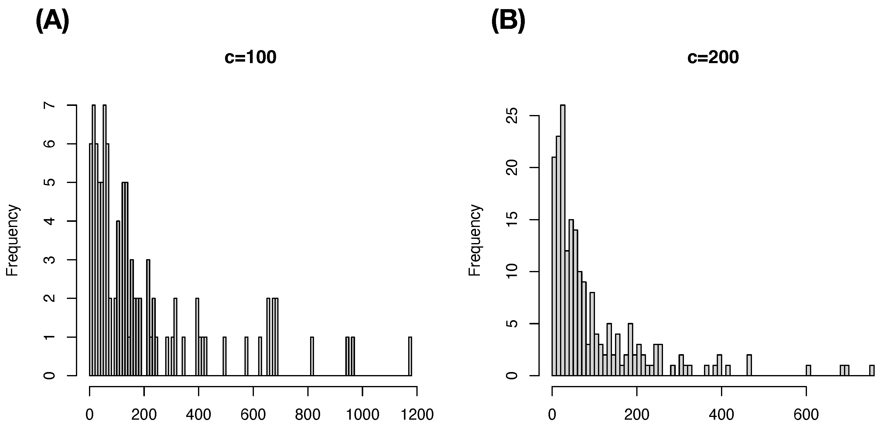
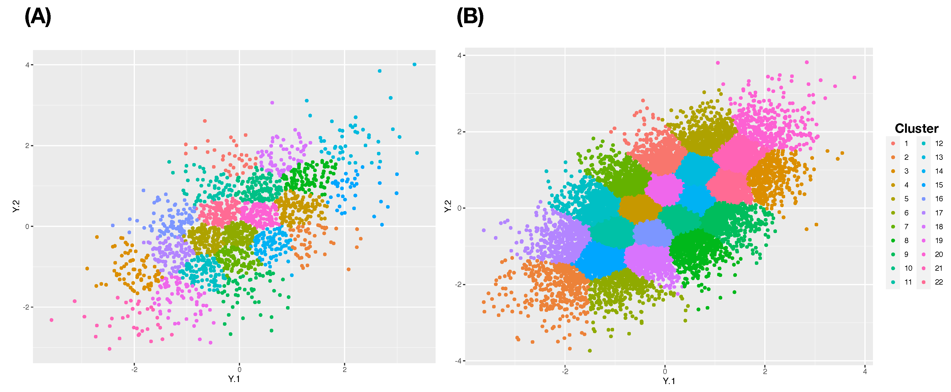
In contrast, we demonstrate that the cluster-based approaches are potentially reasonable choices to mend this effect of the curse of dimensionality. Consider two commonly used clustering algorithms: Hierarchical clustering (HC) and K-means algorithms. It is also known that the HC algorithm is computationally more costly than the K-means algorithm. Since the HC-algorithm heavily relies on a distance matrix, HC-algorithm has difficulties in handling a data set with a very large sample size. Recently, very effective computing packages have been developed for K-means algorithm, that is, K-means algorithm can be effectively applied. On top of computing efficiency differences, there exists a critical difference between the two algorithms. The K-means provides much more even cluster-sizes than HC-algorithm does as illustrated in
Figure 1, see also
Figure 2. For these reasons, we employ K-means clustering, not Hierarchical clustering (HC), algorithm in the following series cases with
.
In this experiment, we take and under two settings with and 20,000. It is noted that the differences in values imply the differences in distribution shapes. The series of clustering compositions are constructed as follows. We apply the K-means algorithm to derive a series of clustering compositions with 12, 22, 32 and 102 clusters. Correspondingly, we built a series of contingency tables of the formats: (1) ; (2) ; (3) and (4) . With respect to the series of clustering compositions, we compute and and . Here, is again the categorical variable of population-IDs.
The messages derived from Example-1 are also observed in Example-2 across 2D to 4D settings in
Table 2,
Table 3 and
Table 4. These results clearly indicate that distribution shape differences can be effectively and reliably picked up by entropy-based evaluations of mutual information between the
Y and categorical label variable
. These results imply that we widely extend one-way ANOVA and two-way ANOVA settings to accommodate high dimensional data points as we have argued in Example-1.
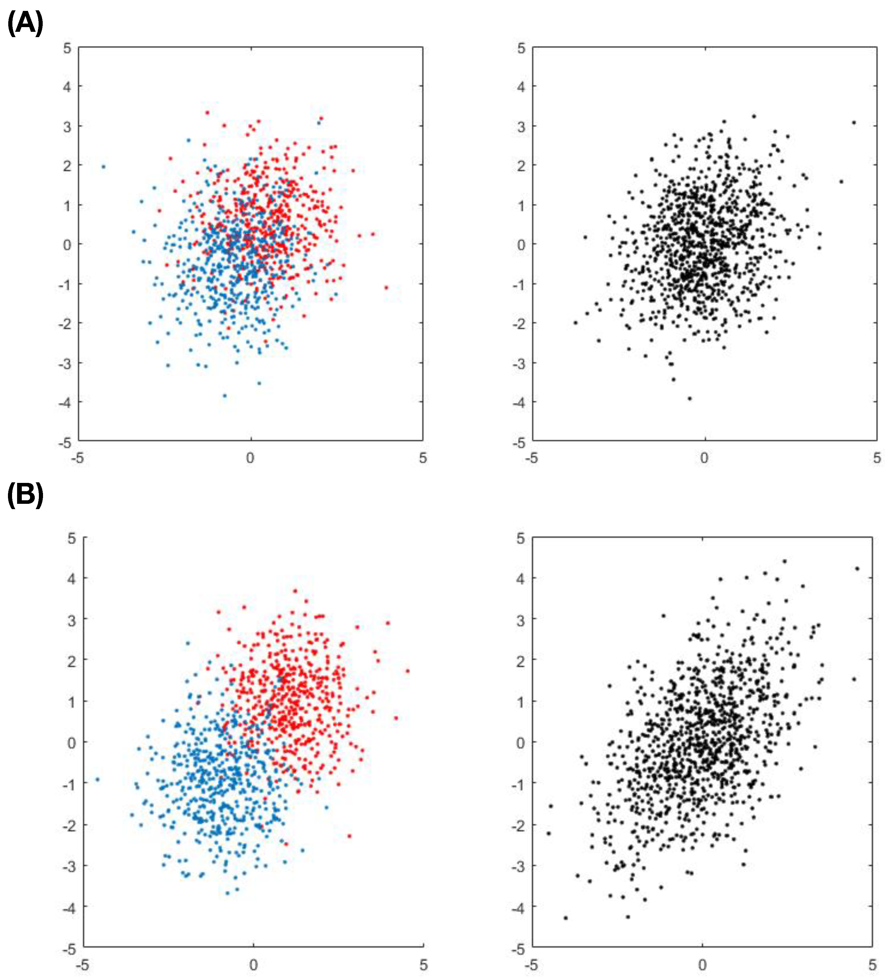
In order to better understand the limit of such an entropy-based approach, we twist the 2D setting in Example-2 a little bit. This more complicated version of Example-2, denoted as Example-
, consists of one 2D normal mixture and one 2D normal. These two 2D distributions are further made to have equal mean vector and covariance matrix. Furthermore, two kinds of mixture-settings are designed and used. The first setting of Example-
is designed for a mixture of two relatively close 2D normals with mean vectors:
and
. The second setting is designed for a relatively apart normal mixture with mean vectors:
and
. These two settings of pairwise scatter-plots are given in
Figure 3. It is obvious that we can visually separate the two 2D distributions in the second mixture setting, but can not do equally well in the first mixture setting.
The mutual information estimates and confidence ranges under the null hypothesis are calculated and reported in
Table 5. In the first mixture setting, it is apparent that
fails to be a major factor by failing to satisfy the criterion [C1: confirmable] across all
K choices. This result is coherent with our visualization through the upper panel
Figure 3. As for the 2nd mixture setting,
is claimed as a major factor by satisfying the [C1: confirmable] criterion across all
K choices. This result is also coherent with our visualization through the lower panel
Figure 3. Further, we observe that the relative position of
estimates against upper and lower limits of null confidence ranges are rather stable when the sizes of clusters are not too small. This observation indeed provides us with the practical guideline for varying choices of
K according to different sample sizes when we employ mutual information to perform inferences under Re-Co dynamics.
We conclude this Example-2 (Example-) with a summarizing statement: Though, any theoretical evaluations of mutual information under the presence of high dimensionality are practically impossible, clustering algorithms provide practical guidelines for building contingency tables and evaluating mutual information for inferential purposes by lessening the effects of curse of dimensionality.
2.3. [Example-3]: From Linear to Highly Nonlinear Associations
We then turn to consider the simplest one-sample problem involving dependent 2D data points. The framework of Re-Co dynamics is self-evident. In this example, we examine the validity and performances of inferences based on estimated mutual information between two 1D continuous random variables
Y and
X via contingency tables of various dimensions. For simplicity in the first scenario of Example-3, we consider a bivariate normal
with covariance matrix:
Here the correlation coefficient
is taken to be
and
, respectively, in this experiment with
or 10,000. The contingency tables are derived from the K-means algorithm being applied on
X and
Y, respectively, with a series of pre-determined numbers of clusters:
.
For the setting of
, we report the calculated
and confidence range of
in
Table 6 across the 16 dimensions of contingency tables. The smallest size of the contingency table has
cells. Its average cell-count is less than 14 for
. The largest size of the contingency table is
, which is more than
. Its averaged cell-count is less than 2 for
20,000.
From the upper half of
Table 6 for the
, all estimates of
are beyond the upper limit of
confidence range of
. That is, the hypothesis of
Y and
X being independent is falsely rejected. In contrast, from the lower half of
Table 6 for the
20,000, all estimates of
are either below the lower limit of
confidence interval of
or within confidence range, except the results based on the largest
contingency table. That is, the same independence hypothesis would not be falsely rejected except in the case of the largest contingency table. Such a contrasting comparison between the upper and lower halves of
Table 6 clearly indicates that validity of mutual information evaluations heavily rely on degrees of volatility of cell counts, especially on testing independence. We further explicitly express such volatility below.
A simple reasoning for the above results goes as follows. For this independent setting of Y and X, for expositional simplicity, let all cells in contingency tables have equal probability. In the smallest contingency table, the cell probability is . The cell-count is a random variable with mean and variance being very close to as well. Thus, the cell-count is falling between with at least . With , the range is close to , while with 20,000 the range is close to . Based on these two intervals, we can see that the Shannon entropy along each row of the contingency table can be volatile with , while it is not the case with 20,000. In fact, when , a contingency table indeed provides much more stable evaluations of mutual information.
In the setting of
, we report the calculated
and confidence range of
in
Table 7 across the 16 dimensions of contingency tables with
20,000. We observe that the calculated
is far above the upper limit of the confidence interval of
even in the largest contingency table with dimension
. The reason is that the number of effectively occupied cells are much smaller due to the dependency, that is, many cells supposed to be empty are indeed empty. With many empty cells coupling with many occupied cells with relatively large cell counts, the Shannon entropy is evaluated with great stability. These results from independent and dependent experimental cases are learned to constitute practical guidelines for evaluating mutual information.
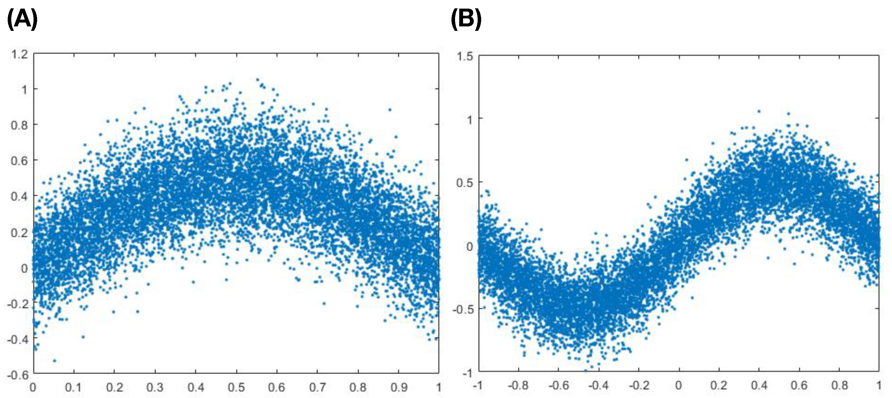
The second scenario of Example-3 is about whether the calculated mutual information
can reveal the existence of non-linear association between
Y and
X. We generate two simulated data sets based on two non-linear associations: (1) half-sine function; (2) full-sine function, as shown in the two panels of
Figure 4. Within both cases of non-linear associations, it is noted that the correlations of
Y and
X are basically equal to zero.
In the setting of a half-sine functional relation, we report the calculated
and confidence range of
in
Table 8 across the 16 dimensions of contingency tables with
20,000. Across all 16 dimensions of contingency tables, the calculated
are far beyond the upper limits of confidence intervals of
. As far as p-value being concerned, they are all basically zeros. The same results are observed in the setting of full-sine functional relations as reported in
Table 9. These two settings in this non-linear association scenario together demonstrate that the calculated
can reveal the existence of significant association between
Y and
X. This demonstration is important in the sense of without knowing the functional forms of their association.
We summarize the practical guidelines that we learned from Example-1 through Example-3 in this section. The most apparent fact is that the calculated values of mutual information vary with respect to dimensions of contingency tables. However, the good news is that the amounts of variations are relatively small and even very minute when cell-counts in the contingency table are not too low. Nonetheless, the calculated mutual information is very capable of revealing the presence and absence of associations underlying Re-Co dynamics of response variable Y and covariate variable X from the three examples and scenarios considered in this section. And it is a reliable way of seeking consistent inferential decisions by varying contingency tables’ dimensions. This capability can be made very efficient if we choose the dimension of the contingency table to suitably reflect the total sample size of the data set with varying degrees. That is, we make sure such efficiency is achieved by varying the dimensions of contingency tables from small to reasonably large. The final guideline is that comparability between two mutual information evaluations is resting on their more or less identical computational platforms, that is, their contingency tables are more or less the same in dimensions. On the other hand, the averaged numbers of cell counts are relatively large, and mutual information evaluations are rather robust to some degree of differences in contingency tables’ dimensions. These practical guidelines will ascertain mutual information evaluations always coupled with reliability. Finally, the data-types of Y and X are entirely free because we rely on their categorical nature only.
5. Conclusions
The most fundamental concept underlying all practical guidelines we have learned from the series of increasingly complex examples in this paper is: the comparability of evaluations of conditional entropy and mutual information critically rests on the equality of the dimensions of the contingency tables where these evaluations are carried out. Based on this comparability concept, the focal goal of the data analysis is then rephrased in terms of [C1: confirmable] criterion regrading presence and absence of major factors underlying a designated Re-Co dynamics. In other words, it is absolutely essential to note that there is no need for precise theoretical information measurements in real data analysis. Such [C1: confirmable] criterion pertaining to the discovery of major factor subsequently promotes all practical guidelines being centered around the task of confirming and debunking an existential collection of major factors of various orders. Since the presence and absence of such an existential collection of major factors indeed manifest the data’s authentic information content, from a data’s information content perspective, the task of data analysis as a whole is translated into the single issue of major factor selection.
Furthermore, all practical guidelines on evaluating mutual information, in particular, for our major factor selection protocol are largely recognized for ascertaining the [C1: confirmable] criterion against the effects of the curse of dimensionality or finite sample phenomenon. Practically, we learn to be sensitively aware of dangers of having low cell-counts in potentially occupied cells when evaluating entropy measures. We also develop clustering-based approaches to lessen the effect of the curse of dimensionality. After learning all these practical guidelines, we are confident in our applications of our major factor selection protocol and related Categorical Exploratory Data Analysis (CEDA) techniques on analyzing real-world structured data sets.
In many scientific fields, like biology, medicine, psychology and social sciences, many measurements are not always precisely metric. Even within a metric system, a continuous measurement is often grouped and converted into a discrete or even ordinal data format. That is, very fine-scale details of a data point is likely given up because it is either too costly to measure, or even can’t be measured, or needs to be discarded for practical computational considerations. Therefore, any structured data set is likely consisting of some features having incomparable measurement scales and some features having no scales at all. How to analyze such a data set in a coherent fashion is not at all a simple task. CEDA is a data analysis designed to be coherent with all features’ measurements. So, CEDA and its major factor selection protocol are developed to indeed embrace the ideal concept: Each single feature must allow to contribute its own authentic information locally, and then to congregate and weave patterns that reveal heterogeneity on global, median and fine scales levels.
To facilitate and carry out such a fundamental concept of data analysis, CEDA is exclusively resting on one simple fact: All data-types are embedded with the categorical nature. So all pieces of local information derived from all categorical or categorized features must be comparable. All these information pieces can be then woven together for the multiscale heterogeneity. By doing so, there are no man-made assumptions or structures needed in CEDA. So, information brought out by CEDA is authentic. That is, we can be free from the danger of generating misinformation via data analysis involving unrealistic assumptions or structures.
To achieve the aforementioned goals of CEDA via our major factor selection protocol, we definitely need stable and creditable evaluations of conditional entropy and mutual information underlying any targeted Re-Co dynamics of interest. That is why the practical guidelines learned in this paper become essential and significant. On the other hand, these practical guidelines also reveal aspects of flexibility and capability of CEDA and its major factor selection in helping scientists to extract intelligence from their own data sets.
As a final remark, we clearly demonstrate in this paper that, by reframing many key statistical topics in one Re-Co dynamics framework, CEDA and its major factor selection protocol not only can resolve the original data analysis tasks, but also, more importantly, can shed authentic lights on issues related to widely expanded frameworks containing the original statistical topics. This capability manifests the capability of CEDA and its major factor selection protocol for truly accommodating and resolving real-world scientific problems.
Finally, we conclude that the learned practical guidelines for evaluating CE and would allow scientists to effectively carry out CEDA and its major factor selection protocol to extract data’s visible and authentic information content, which is taken as the ultimate goal of data analysis.


