Abstract
In this paper, a penalty virtual element method (VEM) on polyhedral mesh for solving the 3D incompressible flow is proposed and analyzed. The remarkable feature of VEM is that it does not require an explicit computation of the trial and test space, thereby bypassing the obstacle of standard finite element discretizations on arbitrary mesh. The velocity and pressure are approximated by the practical significative lowest equal-order virtual element space pair which does not satisfy the discrete - condition. Combined with the penalty method, the error estimation is proved rigorously. Numerical results on the 3D polygonal mesh illustrate the theoretical results and effectiveness of the proposed method.
1. Introduction
In computational fluid dynamics, in order to simulate fluid flow, the incompressible fluid equation is numerically solved. There are classical finite element methods [1] and finite volume methods [2]. It is well known that the traditional finite element method or finite volume method are based on the known interpolation. They are mostly used in structural meshes or quadrilateral meshes, the requirements of meshes are coordinated in the implementation process, so the smoothness of interpolation functions is difficult to improve, which greatly limits the numerical accuracy. The newly developed virtual element method (VEM) [3,4,5] benefits from not requiring a construction of the basis function explicitly to avoid these difficulties. The virtual element space can be constructed by the degrees of freedom of the interior and boundary of the element, and the function space does not need to be expressed explicitly. Therefore, it can be applied to any polygon (polyhedron) with convex or non-convex vertices, and the change of the number of nodes is not needed to recalculate the basis function. Thus, the mesh selection bears great flexibility in the calculation [6,7,8,9].
Due to its flexibility in mesh processing and avoidance of explicit construction of shape functions, VEMs have been successfully applied to a large number of problems. For example, conforming and non-conforming VEMs are presented for elliptic problems in [10,11]. Furthermore, H(div)-conforming and H(curl)-conforming virtual elements are introduced in [12].
In the application of practical problems, the virtual meta method has also made outstanding contributions [13,14,15]. These were developed in [16,17,18] for conforming virtual elements for elasticity problems. Conforming and non-conforming VEMs for fourth-order problems were presented in [19,20,21,22]. -continuous VEMs for the Cahn–Hilliard equation were presented in [23]. For the Stokes problem, several VEMs emerged, such as flow VEM formulations [24], scatter-free virtual elements [25] and non-conforming-required VEMs [26]. When constructing the virtual element space, these methods use more complex degrees of freedom to solve the Stokes equation. For example, in [25], in addition to the degrees of freedom we use, the degrees of freedom also need the moment of the normal vector outside the unit on the edge, and our method is relatively simple. By combining with the penalty method, we can solve the problem of velocity pressure compatibility encountered in the solution of Stokes equation. For the discretization of higher order problems, a class of -conforming () elements was proposed in [27] to satisfy arbitrary regularity requirements. VEMs for parabolic and hyperbolic problems were also developed. Moreover, parabolic and hyperbolic problems were developed in [28,29], respectively. A plane-wave virtual element method for the Helmholtz problem was proposed in the literature [30]. In [31], Mascotto studied the behavior of the stiffness matrix resulting from the approximation of the two-dimensional Poisson problem via the virtual element method. In addition, the SUPG stabilization of the virtual element formulation for advection–diffusion problems was presented in [32], and the virtual element was studied in [33]. In these references, most of the work focused on conforming VEMs with discrete spaces as subspaces of the original space.
In the finite element approximation, a variety of hybrid finite element algorithms which satisfy the velocity pressure - condition have been deeply studied. This condition makes more ideal finite element space unavailable, such as the lowest equal-order - finite element pairs. In practical scientific calculation, the equal-order velocity–pressure pairs are very practical owing to their simple data structure, small amount of calculation and high accuracy. In addition, they violate the discrete - condition, that is, the compatibility between velocity and pressure space, leading to pressure oscillation. In order to compensate for the lack of stability of the - condition, several stabilized finite element methods for incompressible flows are proposed, such as the penalty method [1], regularization method [34], rich multi-scale method [18], local Gauss integral method [2], and so on. Therefore, it is natural to combine the virtual element method with the penalty method to solve the incompressible flow problem.
The outline of this paper is as follows. In the next section, we provide the theoretical results and related continuous forms of the penalty Stokes equations. Section 3 introduces the virtual element space and the virtual element method. Then, the stability and error results of the penalty virtual element method are given. Finally, the numerical results are provided to verify the theoretical analysis and the effectiveness of the proposed method.
2. The Stationary Penalty Stokes Equations
Let be a polygonal domain in . This paper considers the 3D incompressible Stokes equations to illustrate the penalty virtual element method:
where and p are the velocity field and the pressure field, respectively. represents the external force [35].
The penalty method applied to (1) is to approximate the solution by satisfying the following steady-state penalty Stokes Equation [34]
where the penalty parameter is .
Consider the Hilbert spaces
with norms , .
The Galerkin variational formula of Equation (1): find , namely
where the bilinear forms and be defined by:
It is well known that (see for [2,35]):
- and are continuous, i.e.,
- is coercive, i.e., there exists a positive constant such that
- Moreover, the bilinear form satisfies the - condition: where there exists a constant such that
The variational formula of Equation (2): find such that
where denotes some generic constant depending on the data , which may stand for different values at its different occurrences.
There are the following error estimates [1,34].
Please refer to [1,34] for details of certification.
3. The Penalty Virtual Element Method for Stokes Equations
The model problem (1) where is (for simplicity) a convex polyhedron. We suppose that we are given a decomposition of in rather general polyhedra K. We can assume that satisfies the regularity assumption [5]: ∃ a constant assume that
- each polyhedron is star-shaped with respect to every point of a ball of radius ;
- for every face we have and f is star-shaped with respect to every point of a disk of radius ;
- for every edge , we have
where is the diameter of element K, that is, the maximum distance between two nodes of element K; f is a face of element K; is the diameter of the face f; e is the edge length of the element K.
For , the same discussion as in [10] reveals that the dimension of is
One of the advantages of the virtual element method is that it does not need to display the construction unit basis function, so one of our most important calculation tools is the definition of scale monomials. The form of scale monomials is given below
where is a vector, is a triple index, is the element K diameter, and is the element K centroid.
Different from the construction of the two-dimensional (2D) virtual element space, in the case of 2D, the lower order polynomial of polygon cannot be obtained. Therefore, we calculate on the edge of the element and extend it to the whole space by using the boundary value problem. Therefore, the 2D virtual element space mainly considers the nodes, edges and interior of the element. In the construction of the 3D virtual element space, we should not only consider the nodes and interior of the element, but also the nodes, ridge and interior of the face on each face
where . Here is the function space of a face defined in an element K, space is defined on the face , e is an edge of the face , and is all the edges of the face . is the set of polynomials on of degree .
With the definition of the space of a single face , we give the definition of the virtual meta space of all faces
here, is the set of all faces of element K.
The definition of local finite element spaces is given by
For each polyhedron K, we define a local finite element space . Roughly speaking, contains all polynomials of degree k (which is essential for convergence) plus other functions whose restriction on a face is still a polynomial of degree k.
Note that even here a polynomial of degree k satisfies the conditions above, so that is a subspace of . We can take the following degrees of freedom in :
- the value of at the vertices of K;
- on each edge e, the value of at the internal points of the -points Gauss–Lobatto quadrature rule on e;
- for each face f the moments up to order of in f:where the scaled monomials are defined by
- the moments up to order of in K:where the scaled monomials are defined in (1.5), and by
For each polyhedron and , we can construct according to the method in [6], which is defined as follows
where, is a projection operator of constant functions, that we choose as
Remark 1.
Note that, integrating by parts, we have again, for every ,
Since , the first term can again (for ) be computed using the degrees of freedom (iv). The second term, instead, cannot be computed directly from the degrees of freedom (iii), since on each face f of , is in , but the choice of using allows us to compute the moments of order k-1 and k as well. It is known in [5]: When constructing - projection operator, the shape function on every polygon K is in the space . For any and the degree of freedom of given shape function , the moments up to order k can be calculated accurately.
However, there only exists the -projection on all polyhedrons of degree no more than in , which is not enough to deal with more complex situations, e.g., the -error estimates and lower-order terms. To this end, the modified virtual element spaces on every face element K.
The -orthogonal projection , and for any ,
For each polyhedron K, a local finite element space is defined. Now, the local virtual element spaces for the velocity and pressure are, respectively, introduced by
Then, we can define the global finite element space as
3.1. Constructing the Discrete Matrix
With the definition of -projection operator, we first define the local discrete version for (4). The discrete version of is set as
where is any symmetric, positive definite and computable bilinear form that guarantees [5]:
Then, it is easy to prove that this discrete local bilinear form satisfies the following consistency and stability assumptions [36]:
- k-compatibility: if , have
- Stability: there are two positive constants and dependent on and K, have
- Computability: we can know the computability of the discrete bilinear form from Remark 1.
Finally, we define the global approximated bilinear form by simply summing the local contributions
We define projection . The bilinear form and global contributions are given as
The linear form on the right-hand side of the variational problem is discrete by such that
The first term in is the penalty term, and the second term is the stable term.
3.2. Theoretical Analysis
We begin by proving an approximation result for the virtual local space . First of all, let us recall a classical result by Scott–Dupont [37].
Lemma 2.
Let , then for all with , there exists a polynomial function , such that
We have the following proposition
Proposition 1.
Let with . Under the mesh assumptions, there exists a polynomial function , such that
where C is a constant independent of h, and denotes the “diamond” of K, i.e., the union of the polygon in intersecting K.
Lemma 3.
Given the discrete spaces and defined in (2.3) and (2.4), there exists a positive β, independent of h, such that: the bilinear form satisfies the discrete - condition, i.e.,
Proof.
We only sketch the proof, because it essentially follows the guidelines of Theorem 3.1 in [38]. Since the continuous inf-sup condition (2.6) is fulfilled, it is sufficient to construct a linear operator , satisfying
where is a positive h-independent constant. Given , using arguments borrowed from [38] and considering the VEM interpolant presented in Proposition (4.1), we first construct such that
and
□
Thus, we can directly have the following two lemmas with analogous proof as in [37], which are omitted here.
Lemma 4.
There exists a positive constant C such that, for all and all smooth enough functions φ defined on K, it holds:
Define a norm as . We have the following theorem.
Theorem 2.
Proof.
Combined with the definition of projection operator , , . When , , is the component of (references [4,5]). Firstly, we simply deal with and ,
Next, using the above notation and k-consistency, we obtain
According to Lemmas 3 and 4, we have
Combined with Equation (16), we can obtain the estimation formula of
Similarly, we can do the same with
Thirdly, apply the properties of the defined projection operator to obtain
combining (19) and applications of the triangle inequality, this proof is completed. □
4. Numerical Experiments
In this section, we will present the results of three numerical experiments to illustrate some of the characteristics of the methods discussed in the previous sections. In the first experiment, we used arbitrary hexahedral mesh to verify the effectiveness and convergence of the method. In the second numerical experiment, we used mesh generation with suspension points and polyhedral mesh. In the third experiment, we considered square cavity flow without true solution. In addition, the meshes we use are divided in the cube area of .
We use projectors and to evaluate the error:
- -norm: ;
- -norm: .
4.1. Smooth Solution
We consider the parabolic Equation (1), where the load term and the Dirichlet boundary are chosen according to the exact solution with
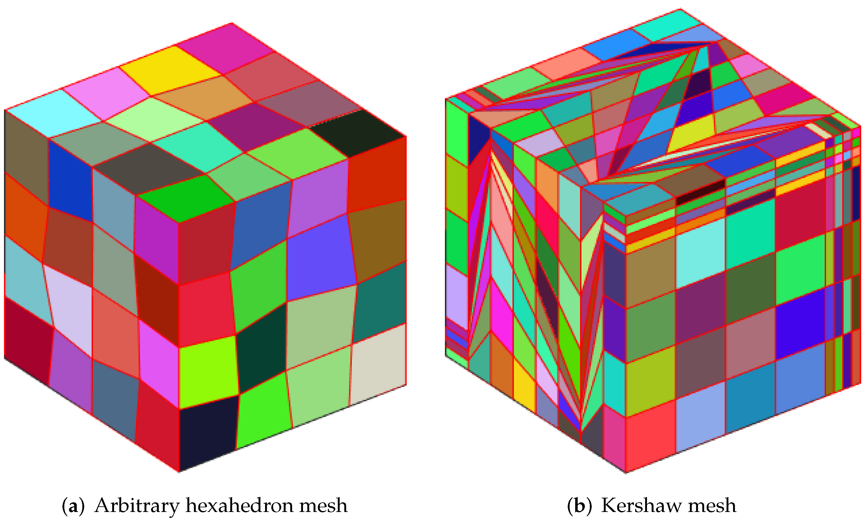
The corresponding results are shown in Table 1, where we use arbitrary hexahedron mesh and Kershaw mesh in Figure 1. Table 1 shows the and and when . It can be seen from the table that the and can reach the order 1, and the can reach the order 2, which is consistent with our theoretical results.

Table 1.
Error results with arbitrary hexahedron mesh and Kershaw mesh.

Figure 1.
Polyhedral mesh.
4.2. True Solution
Let us provide a numerical example. The solution domain is set as . The exact solution for the velocity is generated by , where
and the pressure is given by
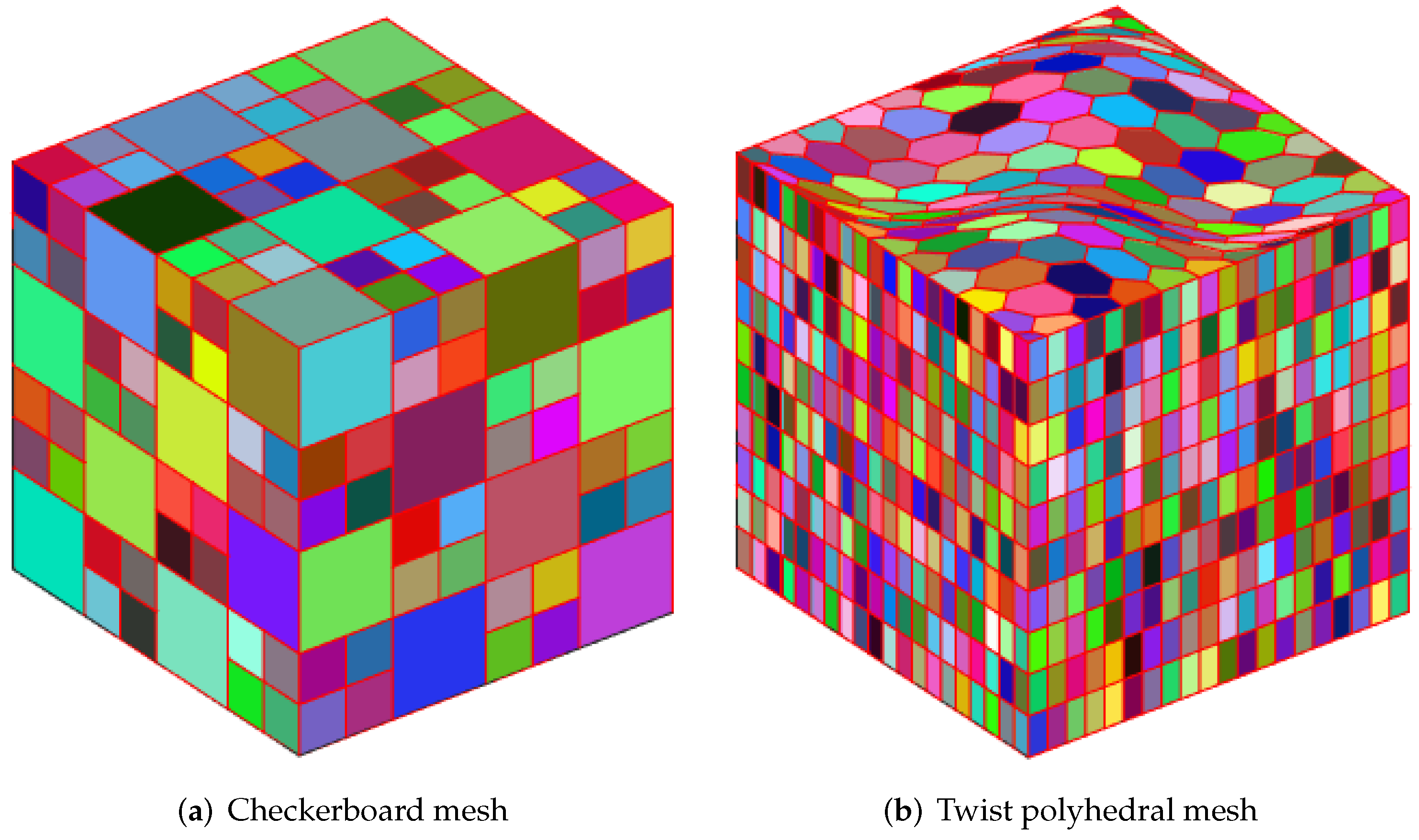
Through this numerical experiment, we can see from Table 2 that our method is still valid for mesh with hanging points Figure 2a. In addition, for twist polyhedral mesh Figure 2b, our method can reach the theoretical order.
Table 2.
Error results with checkerboard mesh and twist polyhedral mesh.
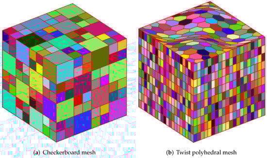
Figure 2.
Polyhedral mesh.
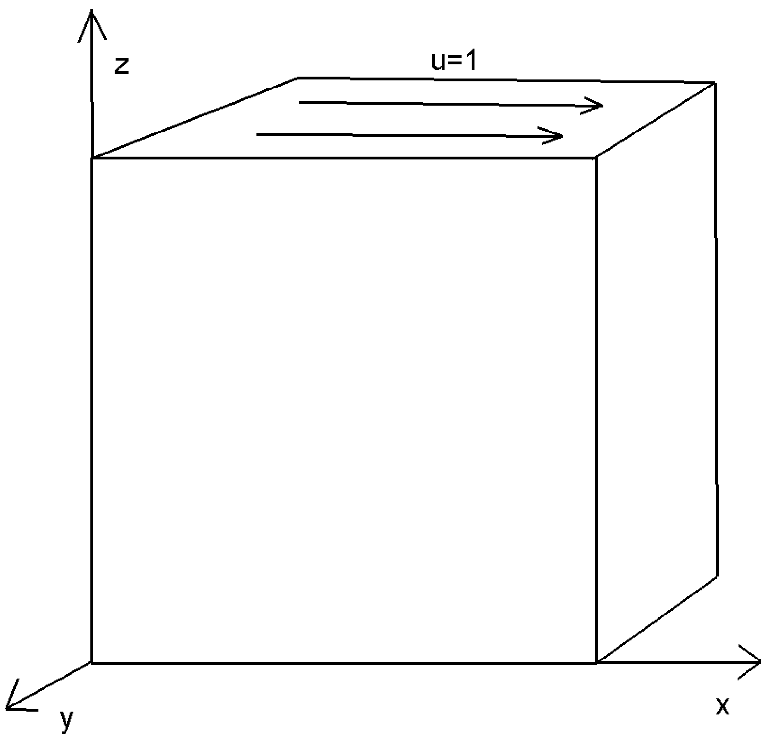
4.3. Driven Cavity Flow
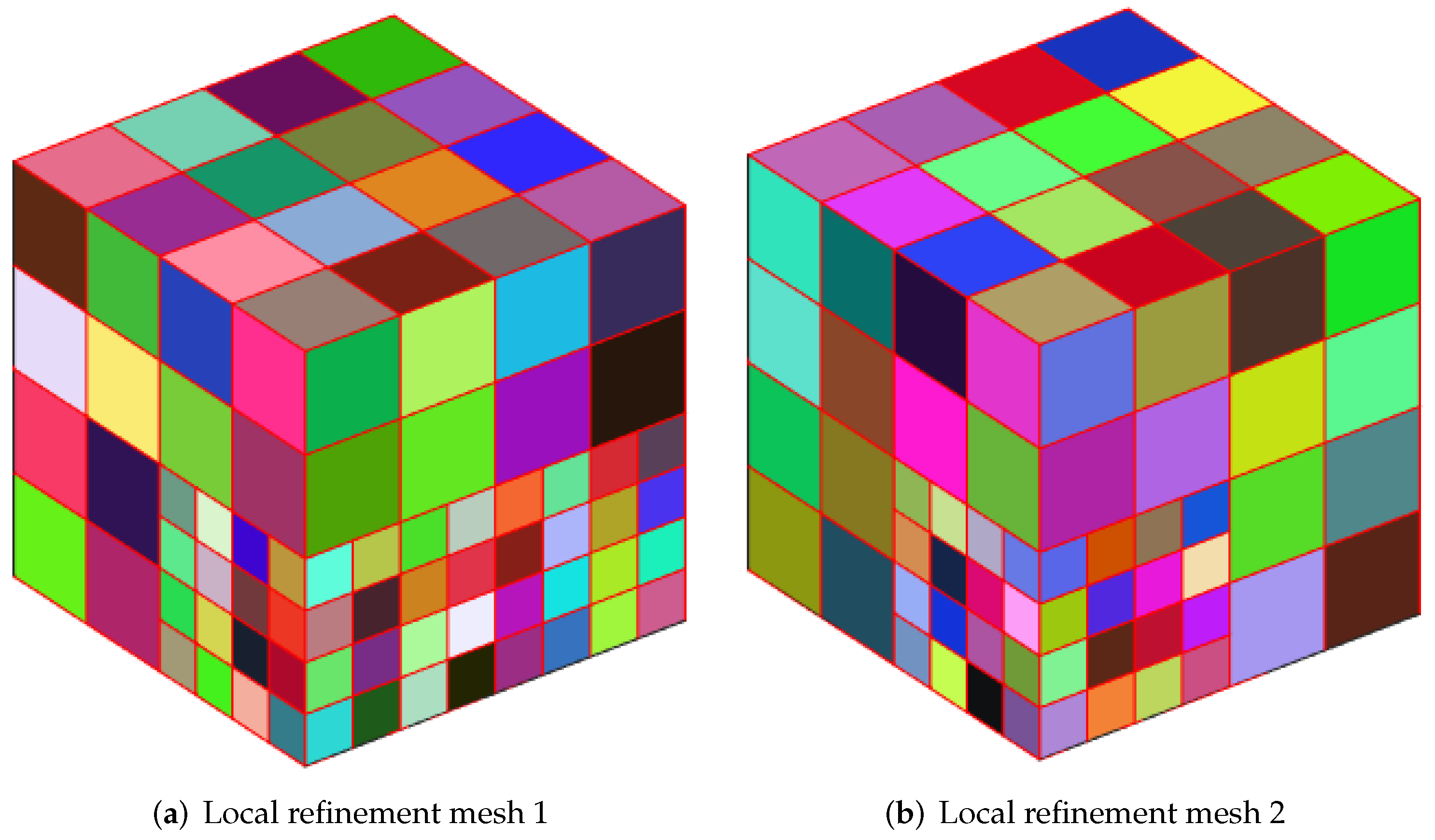
We employ a cubic cavity flow to illustrate the feasibility of the 3D Stokes flows. Consider a cube per unit volume here. In this numerical example, the unit tangential velocity in the x-direction is prescribed on the top surface (), and is prescribed on the remaining bounding surfaces, see Figure 3. The experiments of driven cavity flow are mainly carried out on locally refinement mesh to verify that our method is effective for mesh with hanging points (see Figure 4).

Figure 3.
Cubic cavity flow problem with boundary conditions.
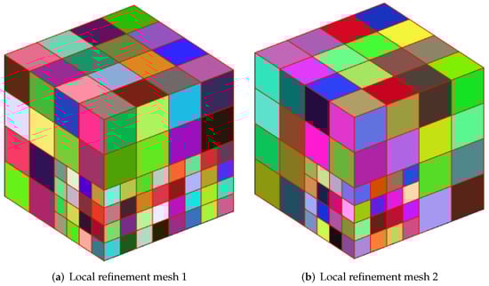
Figure 4.
Polyhedral mesh.
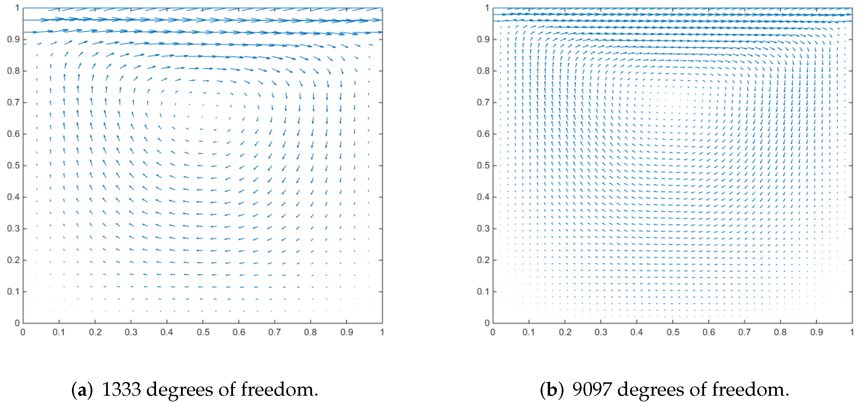
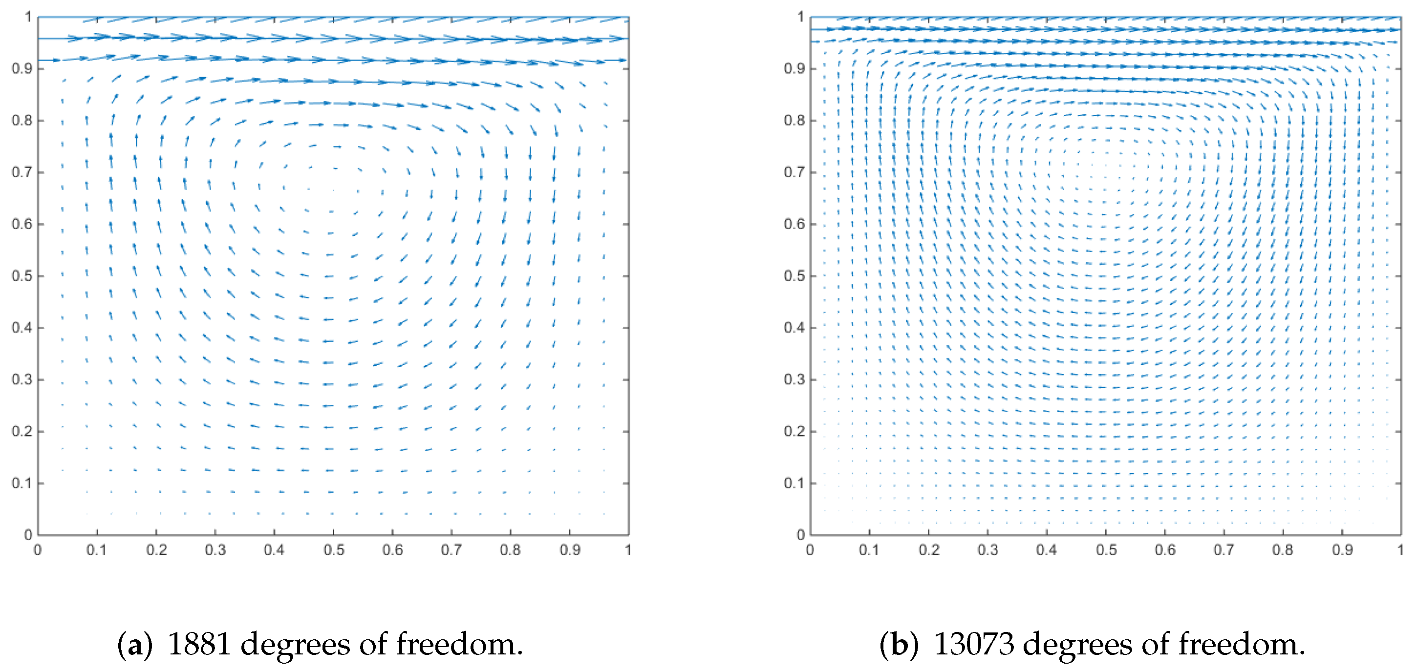
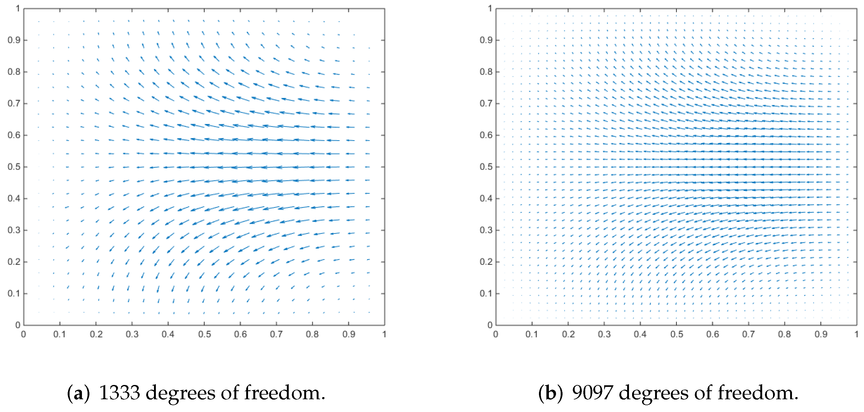
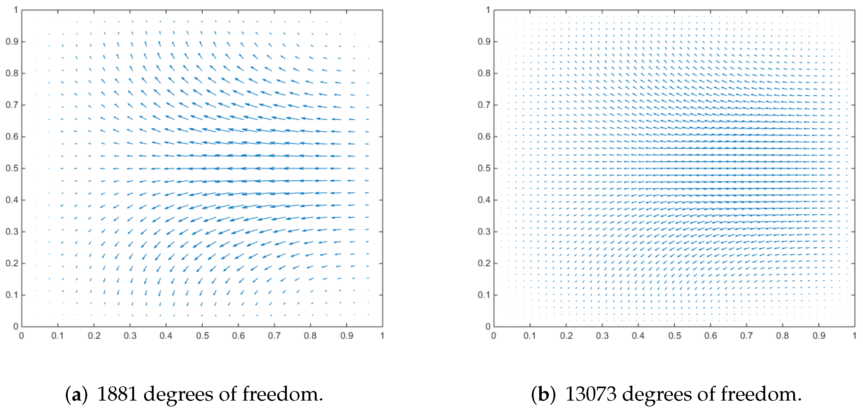
Figure 5 shows the velocity cross-section of the first locally refined mesh when the degrees of freedom are 1881 and 13,073, and . Figure 6 shows the velocity cross-section of the second locally refined mesh when with 1333 and 9097 degrees of freedom. On the other hand, Figure 7 and Figure 8, respectively, show the velocity vectors of Stokes flow in the X–Y plane with in the two grid cubic cavities. The velocity affects the distribution of the intensity of the vorticity, so we look more closely at the vorticity profile for more cross-sections.
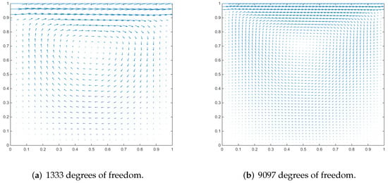
Figure 5.
Velocity vectors of x–z plane at y = 0.5 for Stokes flow in a cubic cavity.
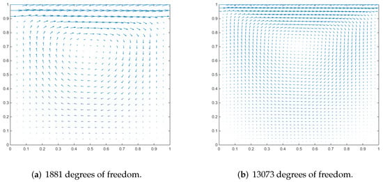
Figure 6.
Velocity vectors of x–z plane at y = 0.5 for Stokes flow in a cubic cavity.
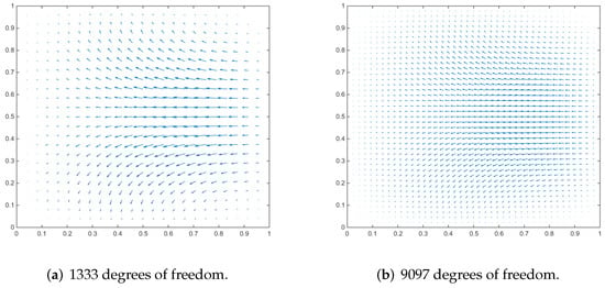
Figure 7.
Velocity vectors of x–y plane at z = 0.5 for Stokes flow in a cubic cavity.
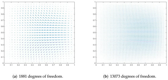
Figure 8.
Velocity vectors of x–y plane at z = 0.5 for Stokes flow in a cubic cavity.
It can be seen that when the degrees of freedom are similar, the cavity flow phenomena under different grids are similar. In the same grid, the phenomena of different degrees of freedom are stable, which shows that our method is effective.
5. Conclusions
In this work, an interesting combination of VEM and the lowest order element with practical significance is proposed for the three-dimensional incompressible flow on polyhedral meshes. In order to better illustrate the method, the optimal error estimate is strictly given by taking the Stokes equation as an example. Numerical experiments verify the theoretical analysis and the effectiveness of the method for arbitrary polyhedral meshes, meshes with hanging points and distorted polyhedral meshes. In our ongoing work, we will consider the adaptive scheme in the VEM framework.
Author Contributions
Conceptualization, Y.H. and H.S.; methodology, H.S. and L.L.; software, L.L.; validation, Y.H. and H.S.; formal analysis, H.S. and L.L.; investigation, H.S. and L.L.; resources, Y.H. and H.S.; data curation, L.L.; writing—original draft preparation, L.L.; writing—review and editing, Y.H., H.S. and L.L.; visualization, L.L.; supervision, Y.H.; project administration, Y.H. and H.S.; funding acquisition, Y.H. All authors have read and agreed to the published version of the manuscript.
Funding
This research received no external funding.
Data Availability Statement
Not applicable.
Acknowledgments
The authors would like to thank the editor and referees for their valuable comments and suggestions, which helped us to improve the results of this paper.
Conflicts of Interest
The authors declare no conflict of interest.
Nomenclature
The following abbreviations are used in this manuscript:
| P | pressure |
| u | dimensionless velocity components |
| penalty parameter | |
| L2-orthogonal projection | |
| H1 projection operator | |
| P | projection operator of constant functions |
| K | polyhedral element |
| f | face of polyhedral element |
| N | dimension of shape function space |
| h | diameter of polyhedral element |
| e | ridge of polyhedral element |
| mesh generation | |
| h | diameter of face of polyhedral element |
References
- Carey, G.; Krishnan, R. Penalty finite element method for the Navier-Stokes equations. Comput. Methods Appl. Mech. Eng. 1984, 2, 183–224. [Google Scholar] [CrossRef]
- Feng, X.; Kim, I.; Nam, H. Locally stabilized P1-nonconforming quadrilateral and hexahedral finite element methods for the Stokes equations. J. Comput. Appl. Math. 2011, 5, 714–727. [Google Scholar] [CrossRef]
- Brenner, S.C.; Scott, L.R. The Mathematical Theory of Finite Element Methods. Texts Appl. Math. 2002, 3, 263–291. [Google Scholar]
- Beirão da Veiga, L.; Lovadina, C.; Vacca, G. Divergence free Virtual Elements for the Stokes problem on polygonal meshes. Mathematics 2015, 2, 327–346. [Google Scholar]
- Brezzi, F.; Falk, R.S.; Marini, L.D. Basic principles of mixed Virtual Element Methods. Esaim Math. Model. Numer. Anal. 2014, 4, 1227–1240. [Google Scholar] [CrossRef]
- Da Veiga, L.B.; Lovadina, C.; Vacca, G. Virtual Elements for the Navier-Stokes Problem on Polygonal Meshes. SIAM J. Numer. Anal. 2018, 3, 1210–1242. [Google Scholar] [CrossRef]
- Cáceres, E.; Gatica, G.N. A mixed virtual element method for the pseudostress—Velocity formulation of the Stokes problem. IMA J. Numer. Anal. 2017, 1, 296–331. [Google Scholar] [CrossRef]
- Cáceres, E.; Gatica, G.N.; Sequeira, F.A. A mixed virtual element method for the Brinkman problem. Math. Model. Methods Appl. Sci. 2017, 4, 707–743. [Google Scholar]
- Liu, X.; Li, J.; Chen, Z. A nonconforming virtual element method for the Stokes problem on general meshes. Comput. Methods Appl. Mech. Eng. 2017, 15, 694–711. [Google Scholar] [CrossRef]
- De Dios, B.; Lipnikov, K.; Manzini, G. The nonconforming virtual element method. ESAIM Math. Model. Numer. Anal. 2016, 3, 879–904. [Google Scholar] [CrossRef]
- Cangiani, A.; Manzini, G.; Sutton, O. Conforming and nonconforming virtual element methods for elliptic problems. IMA J. Numer. Anal. 2017, 3, 1317–1354. [Google Scholar] [CrossRef]
- Da Veiga, L.; Brezzi, F.; Marini, L.; Russo, A. H(div) and H(curl)-conforming virtual element methods. Numer. Math. 2016, 133, 303–332. [Google Scholar] [CrossRef]
- Cascio, M.; Milazzo, A.; Benedetti, I. Virtual element method for computational homogenization of composite and heterogeneous materials. Compos. Struct. 2020, 232, 111523. [Google Scholar] [CrossRef]
- Brenner, S.C.; Sung, L.Y. Virtual element methods on meshes with small edges or faces. Math. Model. Methods Appl. Sci. 2018, 7, 1291–1336. [Google Scholar] [CrossRef]
- Zhang, X.; Chi, H.; Paulino, G. Adaptive multi-material topology optimization with hyperelastic materials under large deformations: A virtual element approach. Comput. Methods Appl. Mech. Eng. 2020, 370, 112976. [Google Scholar] [CrossRef]
- Da Veiga, L.; Brezzi, F.; Marini, L. Virtual elements for linear elasticity problems. SIAM J. Numer. Anal. 2013, 2, 794–812. [Google Scholar] [CrossRef]
- Da Veiga, L.; Lovadina, C.; Mora, D. A virtual element method for elastic and inelastic problems on polytope meshes. Comput. Methods Appl. Mech. Eng. 2015, 295, 327–346. [Google Scholar] [CrossRef]
- Gain, A.; Talischi, C.; Paulino, G. On the virtual element method for three-dimensional linear elasticity problems on arbitrary polyhedral meshes. Comput. Methods Appl. Mech. Eng. 2014, 282, 132–160. [Google Scholar] [CrossRef]
- Antonietti, P.; Manzini, G.; Verani, M. The fully nonconforming virtual element method for biharmonic problems. Math. Model. Methods Appl. Sci. 2018, 2, 387–407. [Google Scholar] [CrossRef]
- Brezzi, F.; Marini, L. Virtual element methods for plate bending problems. Comput. Methods Appl. Mech. Eng. 2013, 253, 455–462. [Google Scholar] [CrossRef]
- Zhao, J.; Chen, S.; Zhang, B. The nonconforming virtual element method for plate bending problems. Math. Model. Methods Appl. Sci. 2016, 9, 1671–1687. [Google Scholar] [CrossRef]
- Zhao, J.; Zhang, B.; Chen, S. The Morley-type virtual element for plate bending problems. J. Sci. Comput. 2018, 1, 610–629. [Google Scholar] [CrossRef]
- Antonietti, P.; Da Veiga, L.; Scacchi, S.; Verani, M. A C1 virtual element method for the Cahn–Hilliard equation with polygonal meshes. SIAM J. Numer. Anal. 2016, 1, 34–56. [Google Scholar] [CrossRef]
- Antonietti, P.; Da Veiga, L.; Mora, D.; Verani, M. A stream virtual element formulation of the Stokes problem on polygonal meshes. SIAM J. Numer. Anal. 2014, 1, 386–404. [Google Scholar] [CrossRef]
- Da Veiga, L.; Lovadina, C.; Vacca, G. Divergence free virtual elements for the Stokes problem on polygonal meshes. ESAIM Math. Model. Numer. Anal. 2017, 2, 509–535. [Google Scholar] [CrossRef]
- Cangiani, A.; Gyrya, V.; Manzini, G. The nonconforming virtual element method for the Stokes equations. SIAM J. Numer. Anal. 2016, 6, 3411–3435. [Google Scholar] [CrossRef]
- da Veiga, L.; Manzini, G. A virtual element method with arbitrary regularity. IMA J. Numer. Anal. 2014, 2, 759–781. [Google Scholar] [CrossRef]
- Vacca, G. Virtual element methods for hyperbolic problems on polygonal meshes. Comput. Math. Appl. 2017, 5, 882–898. [Google Scholar] [CrossRef]
- Vacca, G.; da Veiga, L. Virtual element methods for parabolic problems on polygonal meshes. Numer. Methods Partial. Differ. Equations 2015, 6, 2110–2134. [Google Scholar] [CrossRef]
- Perugia, I.; Pietra, P.; Russo, A. A plane wave virtual element method for the Helmholtz problem. ESAIM Math. Model. Numer. Anal. 2016, 3, 783–808. [Google Scholar] [CrossRef]
- Mascotto, L. Ill-conditioning in the virtual element method: Stabilizations and bases. Numer. Methods Partial. Differ. Equ. 2018, 4, 1258–1281. [Google Scholar] [CrossRef]
- Benedetto, M.; Berrone, S.; Borio, A.; Pieraccini, S.; Scialo, S. Order preserving SUPG stabilization for the virtual element formulation of advection–diffusion problems. Comput. Methods Appl. Mech. Eng. 2016, 311, 18–40. [Google Scholar] [CrossRef]
- Da Veiga, L.; Chernov, A.; Mascotto, L.; Russo, A. Basic principles of hp virtual elements on quasiuniform meshes. Math. Model. Methods Appl. Sci. 2016, 8, 1567–1598. [Google Scholar] [CrossRef]
- He, Y.; Li, J. A penalty finite element method based on the Euler implicit/explicit scheme for the time-dependent Navier-Stokes equations. J. Comput. Appl. Math. 2010, 3, 708–725. [Google Scholar] [CrossRef]
- He, Y.; Li, J. A stabilized finite element method based on local polynomial pressure projection for the stationary Navier-Stokes equations. Appl. Numer. Math. 2008, 10, 1503–1514. [Google Scholar] [CrossRef]
- Chen, L.; Huang, J. Some error analysis on virtual element methods. Calcolo 2018, 1, 1–23. [Google Scholar] [CrossRef]
- Veiga, L.; Brezzi, F.; Marini, L. Virtual Element Methods for general second order elliptic problems on polygonal meshes. Math. Model. Methods Appl. Sci. 2014, 4, 75–89. [Google Scholar]
- Kashiwabara, T.; Oikawa, I.; Zhou, G. Penalty method with P1/P1 finite element approximation for the Stokes equations under the slip boundary condition. Numer. Math. 2016, 4, 705–740. [Google Scholar] [CrossRef]
Publisher’s Note: MDPI stays neutral with regard to jurisdictional claims in published maps and institutional affiliations. |
© 2022 by the authors. Licensee MDPI, Basel, Switzerland. This article is an open access article distributed under the terms and conditions of the Creative Commons Attribution (CC BY) license (https://creativecommons.org/licenses/by/4.0/).