Effective Gibbs State for Averaged Observables

Abstract

We introduce the effective Gibbs state for the observables averaged with respect to fast free dynamics. We prove that the information loss due to the restriction of our measurement capabilities to such averaged observables is non-negative and discuss a thermodynamic role of it. We show that there are a lot of similarities between this effective Hamiltonian and the mean force Hamiltonian, which suggests a generalization of quantum thermodynamics including both cases. We also perturbatively calculate the effective Hamiltonian and correspondent corrections to the thermodynamic quantities and illustrate it with several examples.

1. Introduction

There are a lot of physical models which use averaging with respect to fast oscillations one way or another. For example, many derivations of master equations use secular approximation directly ([1] Subsection 3.3.1), ([2] Section 5.2) or as result [3,4] of perturbation theory with Bogolubov–van Hove scaling [5,6] (see also corrections beyond the zeroth order in [7]). Moreover, there is a wide discussion of the applicability of the rotating wave approximation (RWA) and the systematic perturbative corrections to it in the literature [8,9,10,11,12,13,14,15,16,17]. However, in this work, we consider such averaging not as an approximation but as a restriction of our observation capabilities. In addition, we analyze the thermodynamic equilibrium properties of a quantum system, assuming such restrictions. Due to this averaging, the thermodynamic equilibrium properties can be defined by some effective Gibbs state, which is averaged with respect to these fast oscillations, instead of the exact Gibbs state. Similarly to strong coupling thermodynamics, this effective Gibbs state can be defined by some effective temperature-dependent Hamiltonian, which is an analog of the mean force Hamiltonian (see, e.g., ([18] Chapter 22), [19,20] for recent reviews).

In Section 2, we describe the setup of our problem and develop a systematic perturbative calculation for the effective Hamiltonian. We show that the zeroth and the first term of the expansion coincide with the RWA Hamiltonian and, in particular, are temperature independent. In this point, it is similar to effective Hamiltonians also arising as corrections to the RWA but in dynamical and non-equilibrium problems. The second-order term is temperature-dependent. We show that both this term and its derivative with respect to the inverse temperature are non-positive definite.

In Section 3, we show that this definiteness is closely related to the positivity of the information loss due to the fact that we have access only to the averaged observables discussed above rather than all possible observables. We show that information loss leads to energy loss, which is hidden from our observation. We prove (without perturbation theory) that these losses are always non-negative, but in the leading order, they are defined by the second-order temperature-dependent term in the effective Hamiltonian expansion. Additionally, we prove that exact non-equilibrium free energy is always larger than the free energy observable in our setup. If one assumes that the effective Gibbs state is an exact state, then this difference is also defined by the second-order term of the effective Hamiltonian expansion. At the end of Section 3, we argue that the analogy between our effective Hamiltonian and the mean force Hamiltonian is because they are special cases of the general setup, based on so-called conditional expectations.

To dwell on this analogy, in Section 4, we consider a compound system and the mean force Hamiltonian of one of the subsystems for the effective Gibbs state discussed above. We also give the systematic perturbative expansion for it.

In Section 5, we consider several simple examples to illustrate the results of the previous sections. Namely, we consider two interacting two-level systems, two interacting oscillators and a two-level system interacting with the oscillator. We calculate the effective Hamiltonians for such systems and the information losses due to the restriction to the averaged observables.

Both the effective Hamiltonian we define in this work and the explicit perturbative expansion for it are novel, but such a Hamiltonian has much in common with the mean force Hamiltonian (see the end of Section 3 for a more precise discussion). The main difference consists of the choice of a projector. Thus, our results suggest the possibility to generalize equilibrium quantum thermodynamics to effective equilibrium quantum thermodynamics by different choices of the projector.

2. Effective Hamiltonian

We are interested in equilibrium properties of fast oscillating observables which are in resonance with the free Hamiltonian. We assume that the equilibrium state has the Gibbs form

$${\rho }_{\beta }=\frac{e^{-\beta H}}{Z}$$

(1)

with inverse temperature $\beta >0$ and the Hamiltonian of the form

$$H=H_0+\lambda H_I,$$

(2)

where $H_0$ is a free Hamiltonian and $H_I$ is an interaction Hamiltonian, $\lambda$ is a small parameter.

In addition, we consider the observables which are explicitly time-dependent with very specific time dependence. Namely, they depend on time in the Schrödinger picture as follows

$$X\left(t\right)=e^{-i{H}_{0}t}X{e}^{i{H}_{0}t}$$

(3)

i.e., they depend on time in such a way that they become constant in the interaction picture for the “free” Hamiltonian $H_0$. A widely used example of such an observable is a dipole operator interacting with the classical electromagnetic field in resonance with a free Hamiltonian (see, e.g., [21] Section 15.3.1). In addition, we assume that one could actually observe the long-time averages

$${⟨X\left(t\right)⟩}_{\mathrm{av}}=\underset{T\to +\infty }{lim}\frac{1}{T}{\int }_0^T⟨X\left(t\right)⟩dt,$$

(4)

where $⟨X\left(t\right)⟩\equiv Tr{\rho }_{\beta }X\left(t\right)$. By “long”, we mean long with respect to inverses of non-zero Bohr frequencies, where Bohr frequencies are the eigenvalues of the superoperator $[H_0,·]$ (see, e.g., [4] p. 122). The observation of such long-time averages is usual for spectroscopy setups ([22] Section 4). Moreover, we will further discuss the perturbation theory in $\lambda$, assuming that this averaging is already performed, so this long timescale remains “long” even being multiplied by any power of $\lambda$. Otherwise, one should introduce the small parameter in the averaging procedure as well, which leads to more complicated perturbation theory depending on how the small parameter in the averaging and in the Hamiltonian are related to each other.

Average (4) can be represented as

$${⟨X\left(t\right)⟩}_{\mathrm{av}}=TrX{\tilde{\rho }}_{\beta },$$

(5)

where ${\tilde{\rho }}_{\beta }$ is some effective Gibbs state, which could be calculated as

$${\tilde{\rho }}_{\beta }=\mathcal{P}{\rho }_{\beta },$$

(6)

where

$$\mathcal{P}X=\underset{T\to +\infty }{lim}\frac{1}{T}{\int }_0^T{e}^{i{H}_{0}t}X{e}^{-i{H}_{0}t}dt,$$

(7)

because

$$\begin{array}{cc}\hfill {⟨X\left(t\right)⟩}_{\mathrm{av}}& =\underset{T\to +\infty }{lim}\frac{1}{T}{\int }_0^{T}Tr{e}^{-i{H}_{0}t}X{e}^{i{H}_{0}t}{\rho }_{\beta }dt\hfill \\ \hfill & =\underset{T\to +\infty }{lim}\frac{1}{T}{\int }_0^{T}TrX{e}^{i{H}_{0}t}{\rho }_{\beta }{e}^{-i{H}_{0}t}dt=TrX\mathcal{P}{\rho }_{\beta }.\hfill \end{array}$$

(8)

From the thermodynamical point of view, it is natural to represent this effective Gibbs state in the Gibbs-like form

$${\tilde{\rho }}_{\beta }=\frac{1}{Z}{e}^{-\beta \tilde{H}}$$

(9)

with some effective Hamiltonian $\tilde{H}$ similarly to the mean force Hamiltonian ([18], Chapter 22). Let us remark that we have the same partition function for both exact and effective Hamiltonians due to the fact that $\mathcal{P}$ is a trace-preserving map (see Appendix A) $Tr{e}^{-\beta \tilde{H}}=Tr\mathcal{P}{e}^{-\beta H}=Tr{e}^{-\beta H}$. Let us summarize several properties of the superoperator $\mathcal{P}$ which will be used further (see Appendix A for the proof).

• $\mathcal{P}$ is completely positive.
• $\mathcal{P}$ is a self-adjoint (with respect to trace scalar product $Tr{X}^{†}Y$) projector

  $${\mathcal{P}}^2=\mathcal{P}={\mathcal{P}}^{*}.$$

  (10)
• Let the spectral decomposition of $H_0$ have the form $H_0={\sum }_{\epsilon }\epsilon {\Pi }_{\epsilon }$, where $\epsilon$ are (distinct) eigenvalues of $H_0$ and ${\Pi }_{\epsilon }$ are orthogonal projectors ${\Pi }_{\epsilon }{\Pi }_{{\epsilon }^{\prime }}={\delta }_{\epsilon {\epsilon }^{\prime }}{\Pi }_{\epsilon }$, ${\Pi }_{\epsilon }={\Pi }_{\epsilon }^{†}$. Then,

  $$\mathcal{P}X=\sum _{\epsilon }{\Pi }_{\epsilon }X{\Pi }_{\epsilon }$$

  (11)

  for any matrix X.

For the case of one-dimensional projectors ${\Pi }_{\epsilon }$, superoperator (11) is sometimes called the dephasing operation [23]. In the general case, it is usually called pinching [24], p. 16. It can also be understood as a special case of twirling [25] (with one-parameter group).

Effective Hamiltonian $\tilde{H}$ can be calculated by cumulant-type expansion. Namely, we have the following proposition (see Appendix B for the proof).

Proposition 1.

The perturbative expansion of $\tilde{H}$ has the form

$$\tilde{H}=H_0-{\beta }^{-1}\sum _{n=1}{\lambda }^n\sum _{k_0+\cdots +k_m=n}\frac{{(-1)}^m}{m+1}{\mathcal{M}}_{k_0}\left(\beta \right){\mathcal{M}}_{k_1}\left(\beta \right)\cdots {\mathcal{M}}_{k_m}\left(\beta \right),$$

(12)

where

$${\mathcal{M}}_k\left(\beta \right)={(-1)}^k{\int }_0^{\beta }d{\beta }_1\dots {\int }_0^{{\beta }_{k-1}}d{\beta }_k\mathcal{P}{H}_I\left({\beta }_1\right)\dots H_I\left({\beta }_k\right)$$

(13)

and

$$H_I\left(\beta \right)\equiv e^{\beta H_0}{H}_I{e}^{-\beta H_0}.$$

(14)

In particular, the first terms of the expansion have the form

$$\tilde{H}=H_0-{\beta }^{-1}\lambda {\mathcal{M}}_1\left(\beta \right)-{\beta }^{-1}{\lambda }^2\left({\mathcal{M}}_2\left(\beta \right)-\frac{1}{2}{\left({\mathcal{M}}_1\left(\beta \right)\right)}^2\right)+O\left({\lambda }^3\right).$$

(15)

To make this expansion more explicit, let us represent the interaction Hamiltonian in the eigenbasis of the superoperator $[H_0,·]$ in the same way as it is usually performed for Markov master equation derivation ([1] Subsection 3.3.1)

$$H_I=\sum _{\omega }{D}_{\omega },$$

(16)

where sum is taken over the Bohr frequencies and

$$[H_0,D_{\omega }]=-\omega D_{\omega }.$$

(17)

Moreover, as $H_I$ is Hermitian, then $D_{-\omega }=D_{\omega }^{†}$. Hence, we have the following explicit expressions for ${\mathcal{M}}_k\left(\beta \right)$.

Proposition 2.

If Equations (16) and (17) are held, then

$${\mathcal{M}}_k\left(\beta \right)={(-1)}^k\sum _{{\omega }_1,\dots ,{\omega }_{k-1}}{g}_k(\beta ;{\omega }_1,\cdots ,{\omega }_{k-1})D_{{\omega }_1}\cdots D_{{\omega }_{k-1}}{D}_{-{\omega }_1-\dots -{\omega }_{k-1}},$$

(18)

where

$$\begin{array}{cc}\hfill g_k(\beta ;{\omega }_1,& \dots ,{\omega }_{k-1})=\frac{1}{{\prod }_{k=1}^{n-1}{\sum }_{j=1}^k{\omega }_j}\left(\beta -\sum _{k=1}^{n-1}\frac{1}{{\sum }_{j=1}^k{\omega }_j}\right)\hfill \\ \hfill & -\sum _{p=1}^{n-1}\frac{{(-1)}^p}{\left({\prod }_{m=2}^p{\sum }_{i=m}^p{\omega }_i\right){\left({\sum }_{r=1}^p{\omega }_r\right)}^2\left({\prod }_{k=p+1}^{n-1}{\sum }_{j=p+1}^k{\omega }_j\right)}{e}^{-\beta {\sum }_{i=1}^p{\omega }_i}.\hfill \end{array}$$

(19)

For zero denominators, it should be understood as a limit.

The proof can be found in Appendix C. The first terms of expansion (15) take the form (see Appendix C)

$$\tilde{H}=H_0+\lambda D_0-{\lambda }^2\sum _{\omega \ne 0}\frac{\beta \omega +e^{-\beta \omega }-1}{\beta {\omega }^2}{D}_{\omega }{D}_{\omega }^{†}+O\left({\lambda }^3\right).$$

(20)

Thus, the first two terms are temperature-independent and recover the Hamiltonian in the rotating wave approximation (similarly to effective Hamiltonians for dynamical evolution [26,27])

$$H_{\mathrm{RWA}}=H_0+\lambda D_0.$$

(21)

On the other hand, the next term of expansion (20) is the first temperature-dependent correction to the RWA Hamiltonian. This term is always non-positive definite

$${\tilde{H}}^{\left(2\right)}\equiv -\sum _{\omega \ne 0}\frac{\beta \omega +e^{-\beta \omega }-1}{\beta {\omega }^2}{D}_{\omega }{D}_{\omega }^{†}\le 0$$

(22)

due to the fact that it has the form

$${\tilde{H}}^{\left(2\right)}=-\frac{\beta }{2}\sum _{\omega \ne 0}f\left(\beta \omega \right)D_{\omega }{D}_{\omega }^{†},$$

(23)

where $⟨\psi |D_{\omega }{D}_{\omega }^{†}|\psi ⟩=\left|\right|D_{\omega }^{†}{|\psi ⟩||}^2\ge 0$ for arbitrary $|\psi ⟩$,

$$f\left(x\right)\equiv 2\frac{x+e^{-x}-1}{x^2}$$

(24)

is a positive function $f\left(x\right)>0$ for all real x and $\beta$ is assumed to be positive as we consider the positive temperature (but if one considers a negative temperature, which is possible for finite-dimensional systems, then ${\tilde{H}}^{\left(2\right)}$ becomes non-negative). Moreover, ${\tilde{H}}^{\left(2\right)}$ is a monotone function of temperature, because

$$\frac{\partial }{\partial \beta }{\tilde{H}}^{\left(2\right)}=-\frac{1}{2}\sum _{\omega \ne 0}{f}_1\left(\beta \omega \right)D_{\omega }{D}_{\omega }^{†}\le 0,$$

(25)

where

$$f_1\left(x\right)\equiv 2\frac{1-e^{-x}(1+x)}{x^2}$$

(26)

is also a positive function for all real x. In the next section, we will see that if one averages this result with respect to the effective Gibbs state, then this result becomes closely related to general thermodynamic properties which are valid in all the orders of perturbation theory.

Let us also remark that $\underset{x\to +0}{lim}f\left(x\right)=1$, so for the low temperature limit, i.e., when $\beta \omega \gg 1$ for all non-zero Bohr frequencies, Equation (23) takes the form

$${\tilde{H}}^{\left(2\right)}\approx -\frac{\beta }{2}\sum _{\omega \ne 0}{D}_{\omega }{D}_{\omega }^{†},$$

(27)

i.e., the second-order correction in $\lambda$ is linear in $\beta$.

In the recent literature, there is also rising interest in the ultrastrong coupling limit. Let us remark that ${\tilde{H}}^{\left(2\right)}$ is also the leading order difference between effective Hamiltonians for steady states for the ultrastrong coupling limit conjectured in [28] and the one obtained in [29], if one takes the interaction Hamiltonian as a free Hamiltonian in our notation and vice versa. The perturbative corrections for such steady states are discussed in [30].

3. Effective Hamiltonian as Analog of Mean Force Hamiltonian

The free energy F can be defined by the partition function Z as

$$F=-{\beta }^{-1}lnZ,$$

(28)

where, as it was mentioned before, Z could be defined by the same formula $Z=Tr{e}^{-\beta H}=Tr{e}^{-\beta \tilde{H}}$ both by exact Hamiltonian H and by effective Hamiltonian $\tilde{H}$. If one calculates the entropy and the internal energy by equilibrium thermodynamics formulae

$$S={\beta }^2\frac{\partial F}{\partial \beta },U=\frac{\partial \left(\beta F\right)}{\partial \beta },$$

(29)

then it also obviously does not matter if we use the exact or effective Hamiltonian. For initial temperature-independent Hamiltonian, they also could be calculated as:

$$S=-Tr{\rho }_{\beta }ln{\rho }_{\beta },U=TrH{\rho }_{\beta }.$$

(30)

However, for the effective Hamiltonian, the similar formulae need additional corrections due to its dependence on temperature. Namely,

$$S=\tilde{S}-\Delta S,U=\tilde{U}-\Delta U,$$

(31)

where $\tilde{S}$ and $\tilde{U}$ are defined by the formulae similar to Equation (30)

$$\tilde{S}=-Tr{\tilde{\rho }}_{\beta }ln{\tilde{\rho }}_{\beta },\tilde{U}=Tr\tilde{H}{\tilde{\rho }}_{\beta }$$

(32)

In addition, the corrections have exactly the same form as for the mean force Hamiltonian (see, e.g., [31], Equations (11) and (12))

$$\Delta S=-{\beta }^2{⟨{\partial }_{\beta }\tilde{H}⟩}_{\sim },\Delta U=-\beta {⟨{\partial }_{\beta }\tilde{H}⟩}_{\sim }={\beta }^{-1}\Delta S.$$

(33)

Here, ${⟨·⟩}_{\sim }$ denotes the average with respect to the effective Gibbs state, i.e., ${⟨·⟩}_{\sim }\equiv Tr(·{\tilde{\rho }}_{\beta })$. The derivation of these formulae is exactly the same as for analogous formulae for the mean force Hamiltonian (see ([18], Chapter 22), [32]), because it is valid for an arbitrary temperature-dependent Hamiltonian and is based only on the Feynman–Wilcox formula [33,34,35]

$$\frac{d}{d\beta }{e}^{-\beta \tilde{H}}=-{\int }_0^{t}ds{e}^{-(1-s)\beta \tilde{H}}\left(\frac{d}{d\beta }\left(\beta \tilde{H}\right)\right)e^{-s\beta \tilde{H}}.$$

(34)

Due to the fact that $\mathcal{P}$ is a completely positive trace preserving and unital map ($\mathcal{P}I=I$), the entropy is monotone [36], p. 136 under its action, i.e., $\tilde{S}\ge S$. Thus, $\Delta S\ge 0$ and $\Delta U={\beta }^{-1}\Delta S\ge 0$. $\tilde{S}$ and $\tilde{U}$ could be interpreted as entropy and as energy which are accessible to our observations. Our observable entropy is $\tilde{S}$, but due to our restricted observational capabilities, we have the information loss quantified by $\Delta S$. This information loss comes with energy loss quantified by $\Delta U$ and is hidden from our observations.

For second-order expansion in $\lambda$, we have

$$\Delta S=-{\lambda }^2{\beta }^2{⟨{\partial }_{\beta }{\tilde{H}}^{\left(2\right)}⟩}_{\sim }+O\left({\lambda }^3\right)=-{\lambda }^2{\beta }^2{⟨{\partial }_{\beta }{\tilde{H}}^{\left(2\right)}⟩}_0+O\left({\lambda }^3\right),$$

(35)

where ${⟨·⟩}_0$ is the average with respect to the Gibbs state for the free Hamiltonian. Thus, the non-negativity of $\Delta S$ in the second order of perturbation theory agrees with Equation (25). Moreover, it could be calculated (see Appendix D) by the following formula

$$\Delta S=-{\lambda }^2\beta {⟨{\tilde{H}}^{\left(2\right)}⟩}_0+O\left({\lambda }^3\right)=\sum _{\omega >0}\frac{1-e^{-\beta \omega }}{\beta \omega }{⟨D_{\omega }{D}_{\omega }^{†}⟩}_0+O\left({\lambda }^3\right),$$

(36)

where sum is taken only over the positive Bohr frequencies.

The analogy with Equation (22.6) of ([18] Chapter 22) also suggests the following definition of non-equilibrium free energy in a given state $\rho$

$${\tilde{F}}_{\rho }\equiv {⟨\tilde{H}⟩}_{\mathcal{P}}+{\beta }^{-1}{⟨ln\mathcal{P}\rho ⟩}_{\mathcal{P}}=F+{\beta }^{-1}S\left(\mathcal{P}\rho \right||{\tilde{\rho }}_{\beta }),$$

(37)

where ${⟨·⟩}_{\mathcal{P}}\equiv Tr(\mathcal{P}\rho ·)$ and $S\left(\rho \right|\left|\sigma \right)$ is relative entropy ([36], Chapter 7.1). The only difference from Equation (22.6) of ([18] Chapter 22) consists of the fact that we use averaged state $\mathcal{P}\rho$ instead of $\rho$, which is natural in our setup.

The exact free energy is defined as

$$F_{\rho }\equiv ⟨H⟩+{\beta }^{-1}⟨ln\rho ⟩=F+{\beta }^{-1}S\left(\rho \right||{\rho }_{\beta }),$$

(38)

where $⟨·⟩\equiv Tr(\rho ·)$, which leads to

$$F_{\rho }={\tilde{F}}_{\rho }+\Delta F_{\rho },$$

(39)

where similarly to Equation (33), $\Delta F_{\rho }$ has a definite sign, namely

$$\Delta F_{\rho }={\beta }^{-1}\left(S\right(\rho \left|\right|{\rho }_{\beta })-S(\mathcal{P}\rho \left|\right|\mathcal{P}{\rho }_{\beta }\left)\right)\ge 0$$

(40)

due to monotonicity of the relative entropy under the completely positive map $\mathcal{P}$ ([36], Theorem 7.6). Similarly to $\tilde{S}$ and $\tilde{U}$, ${\tilde{F}}_{\rho }$ can be interpreted as observable free energy and $\Delta F_{\rho }$ as free energy hidden from our observations. As $\Delta F_{\rho }\ge 0$, we are always further from equilibrium than we think based on our restricted measurement possibilities. For example, if our exact non-equilibrium state is ${\tilde{\rho }}_{\beta }$, then it is impossible to distinguish it from ${\rho }_{\beta }$. Thus, its observable free energy coincides with the equilibrium one

$${\tilde{F}}_{{\tilde{\rho }}_{\beta }}=F+{\beta }^{-1}S({\tilde{\rho }}_{\beta }\left|\right|{\tilde{\rho }}_{\beta })=F,$$

(41)

but $\Delta F_{{\tilde{\rho }}_{\beta }}$ is positive as in the general case. Namely, by Equations (37) and (38), we have

$$\Delta F_{{\tilde{\rho }}_{\beta }}={⟨H⟩}_{\sim }-{⟨\tilde{H}⟩}_{\sim }.$$

(42)

As ${⟨H⟩}_{\sim }=TrH\mathcal{P}\rho =TrH\mathcal{P}\mathcal{P}{\rho }_{\beta }=Tr\mathcal{P}\left(H\right)\mathcal{P}{\rho }_{\beta }=Tr{H}_{\mathrm{RWA}}{\rho }_{\beta }={⟨H_{\mathrm{RWA}}⟩}_{\sim }$, then

$$\Delta F_{{\tilde{\rho }}_{\beta }}={⟨H_{\mathrm{RWA}}-\tilde{H}⟩}_{\sim }.$$

(43)

This formula is useful for asymptotic expansion of $\Delta F_{{\tilde{\rho }}_{\beta }}$ as the first two terms of the expansion of $\tilde{H}$ cancel $H_{\mathrm{RWA}}$ and the first non-trivial contribution is of order of ${\lambda }^2$ as in Equation (35). Namely, we have

$$\Delta F_{{\tilde{\rho }}_{\beta }}=-{\lambda }^2{⟨H^{\left(2\right)}⟩}_{\sim }+O\left({\lambda }^3\right)=-{\lambda }^2{⟨H^{\left(2\right)}⟩}_0+O\left({\lambda }^3\right).$$

(44)

Moreover, it is possible to show (see Appendix D) that ${⟨{\partial }_{\beta }{H}^{\left(2\right)}⟩}_0={\beta }^{-1}{⟨H^{\left(2\right)}⟩}_0$, so

$$\Delta U=\Delta F_{{\tilde{\rho }}_{\beta }}+O\left({\lambda }^3\right),\Delta S=\beta \Delta F_{{\tilde{\rho }}_{\beta }}+O\left({\lambda }^3\right).$$

(45)

The analogy with the mean force Hamiltonian can be made more explicit if one notes that the mean force Hamiltonian is closely related to the projector ${\mathcal{P}}^{\prime }={Tr}_B(·)\otimes {\rho }_B$ which is usually used for derivation of Markovian master equations and their perturbative corrections ([1], Subsection 9.1.1).

$${\mathcal{P}}^{\prime }\frac{e^{-\beta H}}{Z}=\frac{1}{Z}{Tr}_B{e}^{-\beta H}\otimes \frac{1}{Z_B}{e}^{-\beta H_B}=\frac{1}{Z_{\mathrm{mf}}}{e}^{-\beta H_{\mathrm{mf}}}\otimes \frac{1}{Z_B}{e}^{-\beta H_B},$$

(46)

where $Z_{\mathrm{mf}}=Z/Z_B$ [19]. Thus, a stricter analog of our effective Hamiltonian should be $H_{\mathrm{mf}}+H_B$ with partition function Z. However, it seems that for operational meaning of the mean force Hamiltonian, the information about $H_B$ is also important, which makes this analog more natural. Nevertheless, importance of information about $H_B$ (not $H_{\mathrm{mf}}$ only) is still discussible [37,38].

From the mathematical point of view, both of these projectors are so-called conditional expectations [39,40,41,42]. They are correspondent to different choices of observable degrees of freedom. This suggests that the mean force Hamiltonian theory could be generalized to arbitrary conditional expectations, and for specific conditional expectation $\mathcal{P}$, it is performed in this work. Thus, it is possible to say that the effective Gibbs state with such generalized projectors define different effective quantum equilibrium thermodynamics.

Let us also mention that similarly to mean force Hamiltonian theory, we assume in our work that the whole system (containing both the system and the reservoir in the mean force Hamiltonian case) is at the same temperature. However, there are possible generalizations of such a setup when the system interacts with two (or more) reservoirs at different temperatures [43]. In such a case, a natural analog of ${\mathcal{P}}^{\prime }$ is a projector ${\mathcal{P}}^{″}={Tr}_{B_1,B_2}(·)\otimes {\rho }_{B_1,{\beta }_1}\otimes {\rho }_{B_2,{\beta }_2}$, where ${\rho }_{B_1,{\beta }_1}$ and ${\rho }_{B_2,{\beta }_2}$ are states of the heat baths with inverse temperatures ${\beta }_1$ and ${\beta }_2$, respectively. The above equations assuming only one temperature, e.g., Equations (28) and (29), are not applicable in this case, but Equations (30)–(32), which are fundamental for our approach, still have their meaning. This suggests that it is possible to generalize the framework presented here to include such a multitemperature case, but it is not fully covered by the approach presented here as the scope of the current paper was focused on the one-temperature case. Nevertheless, we think that it is one of the most promising directions for future study.

4. Mean Force Hamiltonian for Effective Gibbs State

Let us now consider a compound system, consisting of two subsystems A and B. Let us consider subsystem B as “reservoir”. Let us assume that $H_0=H_A\otimes I+I\otimes H_B$. Then, it is possible to define a mean for the Hamiltonian ${\tilde{H}}_{\mathrm{mf}}$ for the effective Gibbs state by the following formula

$${\tilde{\rho }}_{\mathrm{mf}}\equiv {Tr}_B\mathcal{P}{\rho }_{\beta }=\frac{1}{{\tilde{Z}}_{\mathrm{mf}}}{e}^{-\beta {\tilde{H}}_{\mathrm{mf}}},$$

(47)

where ${\tilde{Z}}_{\mathrm{mf}}=\tilde{Z}/Z_B$, $Z_B\equiv {Tr}_B{e}^{-\beta H_B}$. Then, similarly to Proposition 1, it is possible to obtain the perturbative expansion in $\lambda$ for ${\tilde{H}}_{\mathrm{mf}}$ (see Appendix E).

Proposition 3.

The perturbative expansion of ${\tilde{H}}_{\mathrm{mf}}$ in λ has the form

$${\tilde{H}}_{\mathrm{mf}}=H_A-{\beta }^{-1}\sum _{n=1}^{\infty }{\lambda }^n\sum _{k_0+\cdots +k_m=n}\frac{{(-1)}^m}{m+1}{⟨{\mathcal{M}}_{k_0}\left(\beta \right)⟩}_B{⟨{\mathcal{M}}_{k_1}\left(\beta \right)⟩}_B\cdots {⟨{\mathcal{M}}_{k_m}\left(\beta \right)⟩}_B,$$

(48)

where ${⟨·⟩}_B\equiv {Tr}_B(·Z_B^{-1}{e}^{-\beta H_B})$.

Here, ${\mathcal{M}}_k\left(\beta \right)$ can also be calculated by Proposition 2. The first terms of the expansion for ${\tilde{H}}_{\mathrm{mf}}$ have the form

$${\tilde{H}}_{\mathrm{mf}}=H_A+\lambda {⟨D_0⟩}_B-{\lambda }^2\frac{\beta }{2}\left(\sum _{\omega \ne 0}f\left(\beta \omega \right){⟨D_{\omega }{D}_{\omega }^{†}⟩}_B+{⟨D_0^2⟩}_B-{⟨D_0⟩}_B^2\right)+O\left({\lambda }^3\right).$$

(49)

This formula can be made even more explicit if one considers the decomposition of $D_{\omega }$ into sum of eigenoperators of $[H_A,·]$ and $[H_B,·]$, i.e., similarly to Equation (17) introducing $A_{\omega }$ and $B_{\omega }$ such that

$$[H_A,A_{{\omega }_1}]=-{\omega }_1{A}_{{\omega }_1},[H_B,B_{{\omega }_2}]=-{\omega }_2{B}_{{\omega }_2},$$

(50)

where ${\omega }_1$ and ${\omega }_2$ run over all possible Bohr frequencies of the Hamiltonians $H_A$ and $H_B$, respectively. Then, expansion (49) takes the form (see Appendix F)

$$\begin{array}{c}\hfill {\tilde{H}}_{\mathrm{mf}}=H_S+\lambda {⟨B_0⟩}_B{A}_0-{\lambda }^2\frac{\beta }{2}(\sum _{{\omega }_1\ne 0}\left(\sum _{\omega }f\left(\beta \omega \right){⟨B_{{\omega }_1+\omega }{B}_{{\omega }_1+\omega }^{†}⟩}_B\right)A_{{\omega }_1}^{†}{A}_{{\omega }_1}\\ \hfill +\left(\sum _{\omega }f\left(\beta \omega \right){⟨B_{\omega }{B}_{\omega }^{†}⟩}_B-{⟨B_0⟩}_B^2\right)A_0^2)+O\left({\lambda }^3\right),\end{array}$$

(51)

where it is assumed that $f\left(0\right)=1$.

5. Examples

In this section, we consider several examples, and the notations are chosen in such a way as to emphasize the similarity between them. We use these examples to illustrate our formulae, but let us remark that, at least for the first and second model, it is possible to calculate the effective Hamiltonian exactly without perturbation theory; however, it is not the aim of our work. For all these examples, we consider two cases: the off-resonance and the resonance one. In this section, only the results are presented, all the calculations are given separately in Appendix G.

5.1. Two Interacting Two-Level Systems

Let us consider the two interacting two-level systems [44,45] a and b

$$H={\omega }_a{\sigma }_a^{+}{\sigma }_a^{-}+{\omega }_b{\sigma }_b^{+}{\sigma }_b^{-}+\lambda ({\sigma }_a^{-}+{\sigma }_a^{+})(g^{*}{\sigma }_b^{-}+g{\sigma }_b^{+}),$$

(52)

where ${\omega }_a>0$, ${\omega }_b>0$ and ${\sigma }_i^{\pm }$ are usual ladder operators for two-level systems $i=a,b$.

(1) Off-resonance case ${\omega }_a\ne {\omega }_b$.

$$\begin{array}{cc}\hfill {\tilde{H}}_{\mathrm{off}-\mathrm{res}}=& {\omega }_a{n}_a+{\omega }_b{n}_b-{\lambda }^2\frac{\beta }{2}{\left|g\right|}^2(f\left(\beta ({\omega }_a-{\omega }_b)\right)(1-n_a)n_b\hfill \\ \hfill & +f\left(\beta ({\omega }_a+{\omega }_b)\right)(1-n_a)(1-n_b)+f\left(\beta ({\omega }_b-{\omega }_a)\right)n_a(1-n_b)\hfill \\ \hfill & +f\left(\beta (-{\omega }_a-{\omega }_b)\right)n_a{n}_b)+O\left({\lambda }^3\right),\hfill \end{array}$$

(53)

where $n_i\equiv {\sigma }_i^{+}{\sigma }_i^{-}$ are number operators for $i=a,b$. In the leading order, the information loss has the form

$$\Delta S_{\mathrm{off}-\mathrm{res}}={\lambda }^2\beta {\left|g\right|}^2\frac{{\omega }_{a}tanh\frac{\beta {\omega }_a}{2}-{\omega }_{b}tanh\frac{\beta {\omega }_b}{2}}{{\omega }_a^2-{\omega }_b^2}+O\left({\lambda }^3\right).$$

(54)

(2) Resonance case ${\omega }_b={\omega }_a+\lambda \delta \omega$.

$$\begin{array}{cc}\hfill {\tilde{H}}_{\mathrm{res}}=& {\omega }_a{n}_a+{\omega }_b{n}_b+\lambda (g{\sigma }_a^{-}{\sigma }_b^{+}+g^{*}{\sigma }_a^{+}{\sigma }_b^{-})\hfill \\ \hfill & -{\lambda }^2\frac{\beta }{2}{\left|g\right|}^2(f\left(2\beta {\omega }_a\right)(1-n_a)(1-n_b)+f(-2\beta {\omega }_a)n_a{n}_b)+O\left({\lambda }^3\right).\hfill \end{array}$$

(55)

In the leading order, the information loss has the form

$$\Delta S_{\mathrm{res}}={\lambda }^2\beta {\left|g\right|}^2\frac{tanh\frac{{\omega }_a\beta }{2}}{2{\omega }_a}+O\left({\lambda }^3\right).$$

(56)

Let us remark that it does not coincide with the off-resonance case with ${\omega }_b\to {\omega }_a$. Namely, we have

$$\Delta S_{\mathrm{off}-\mathrm{res}}{|}_{{\omega }_b\to {\omega }_a}=\Delta S_{\mathrm{res}}+{\lambda }^2{\left(\frac{\beta \left|g\right|}{2cosh\frac{\beta {\omega }_a}{2}}\right)}^2+O\left({\lambda }^3\right).$$

(57)

Thus, off-resonance averaging leads to larger information loss even in the “resonance” limit than resonance averaging.

5.2. Two Interacting Harmonic Oscillators

Let us consider the two interacting harmonic oscillators

$$H={\omega }_a{a}^{†}a+{\omega }_b{b}^{†}b+\lambda (a+a^{†})(g^{*}b+g{b}^{†}),$$

(58)

where ${\omega }_a>0$, ${\omega }_b>0$ and $a,a^{†}$ and $b,b^{†}$ are oscillator (bosonic) ladder operators. Averaging with respect to fast oscillations needed for so-called quasi-stationary states was recently discussed in [46].

(1) Off-resonance case ${\omega }_a\ne {\omega }_b$.

$$\begin{array}{cc}\hfill {\tilde{H}}_{\mathrm{off}-\mathrm{res}}=& {\omega }_a{n}_a+{\omega }_b{n}_b-{\lambda }^2\frac{\beta }{2}{\left|g\right|}^2(f\left(\beta ({\omega }_a+{\omega }_b)\right)(1+n_a)n_b\hfill \\ \hfill & +f\left(\beta ({\omega }_a+{\omega }_b)\right)(1+n_a)(1+n_b)+f\left(\beta ({\omega }_b-{\omega }_a)\right)n_a(1+n_b)\hfill \\ \hfill & +f\left(\beta (-{\omega }_a-{\omega }_b)\right)n_a{n}_b)+O\left({\lambda }^3\right),\hfill \end{array}$$

(59)

where $n_a\equiv a^{†}a$, $n_b\equiv b^{†}b$. In the leading order, the information loss has the form

$$\Delta S_{\mathrm{off}-\mathrm{res}}={\lambda }^2\beta {\left|g\right|}^2\frac{{\omega }_{a}coth\frac{\beta {\omega }_b}{2}-{\omega }_{b}coth\frac{\beta {\omega }_a}{2}}{{\omega }_a^2-{\omega }_b^2}+O\left({\lambda }^3\right).$$

(60)

(2) Resonance case ${\omega }_b={\omega }_a+\lambda \delta \omega$.

$$\begin{array}{cc}\hfill {\tilde{H}}_{\mathrm{res}}=& {\omega }_a{n}_a+{\omega }_b{n}_b+\lambda (ga{b}^{†}+g^{*}{a}^{†}b)\hfill \\ \hfill & -{\lambda }^2\frac{\beta }{2}{\left|g\right|}^2(f\left(2\beta {\omega }_a\right)(1+n_a)(1+n_b)+f(-2\beta {\omega }_a)n_a{n}_b)+O\left({\lambda }^3\right).\hfill \end{array}$$

(61)

In the leading order, the information loss has the form

$$\Delta S_{\mathrm{res}}={\lambda }^2\beta {\left|g\right|}^2\frac{coth\frac{{\omega }_a\beta }{2}}{2{\omega }_a}+O\left({\lambda }^3\right).$$

(62)

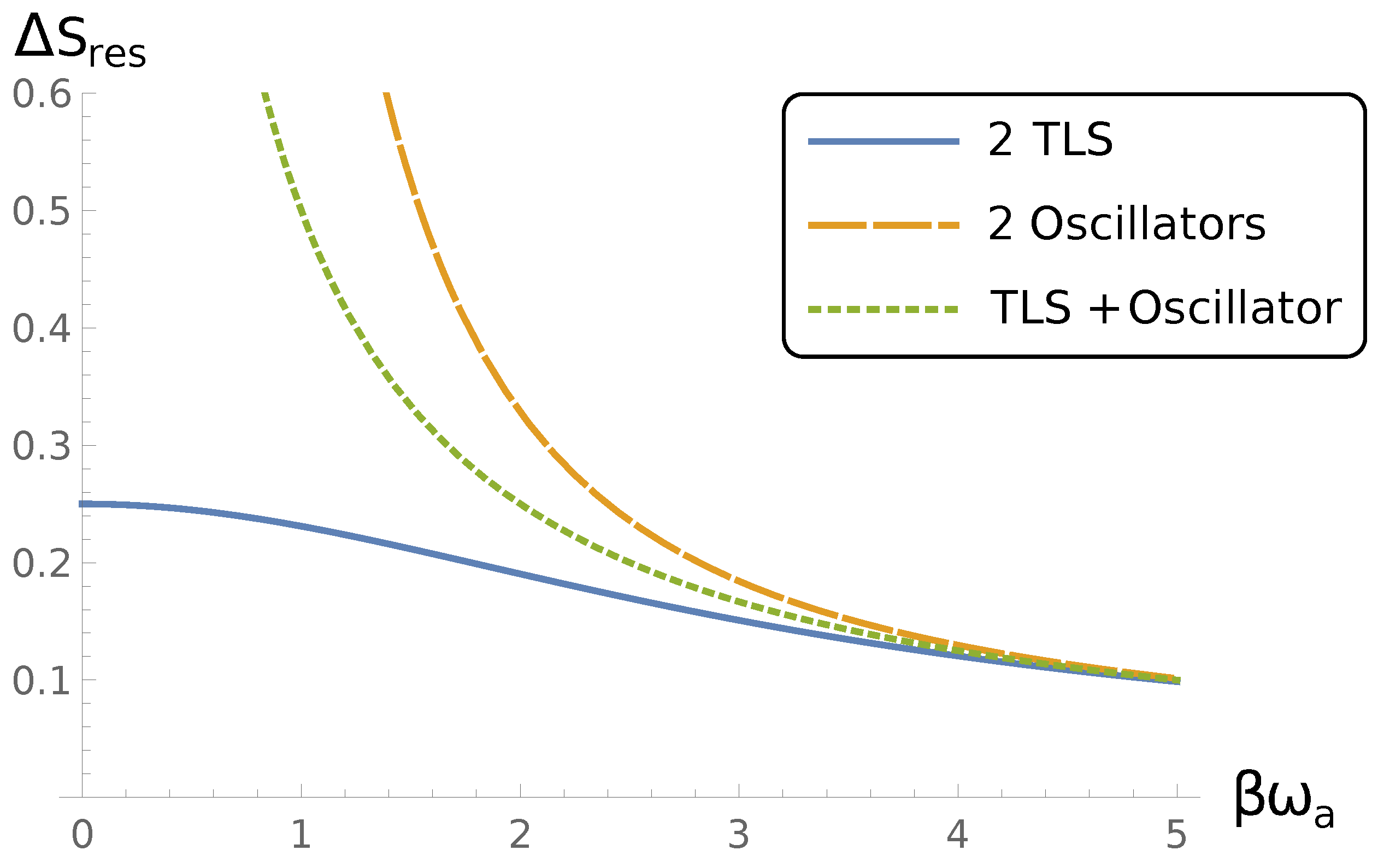
Interestingly, this quantity asymptotically coincides with Equation (56) for ${\omega }_a\beta \gg 1$ (see Figure 1). Similarly to Equation (57), we have

$$\Delta S_{\mathrm{off}-\mathrm{res}}{|}_{{\omega }_b\to {\omega }_a}=\Delta S_{\mathrm{res}}+{\lambda }^2{\left(\frac{\beta \left|g\right|}{2sinh\frac{\beta {\omega }_a}{2}}\right)}^2+O\left({\lambda }^3\right).$$

(63)

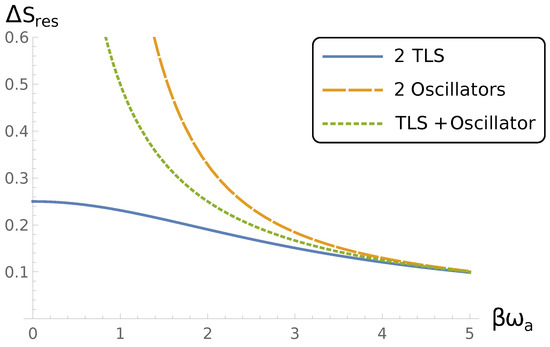
Figure 1. The information loss for resonance case and $\beta \left|g\right|=1$ for two two-level systems (solid line), two oscillators (dashed line) and two-level system interaction with oscillator (dotted line).

5.3. Two-Level System Interacting with Harmonic Oscillator

Let us consider a two-level system interacting with a harmonic oscillator

$$H={\omega }_a{\sigma }^{+}{\sigma }^{-}+{\omega }_b{b}^{†}b+\lambda ({\sigma }^{+}+{\sigma }^{-})(g^{*}b+g{b}^{†}),$$

(64)

where ${\omega }_a>0$, ${\omega }_b>0$ and ${\sigma }^{+},{\sigma }^{-}$ and $b,b^{†}$ are two-level and bosonic ladder operators, respectively.

(1) Off-resonance case ${\omega }_a\ne {\omega }_b$.

$$\begin{array}{cc}\hfill {\tilde{H}}_{\mathrm{off}-\mathrm{res}}=& {\omega }_a{n}_a+{\omega }_b{n}_b-{\lambda }^2\frac{\beta }{2}{\left|g\right|}^2(f\left(\beta ({\omega }_a+{\omega }_b)\right)(1-n_a)n_b\hfill \\ \hfill & +f\left(\beta ({\omega }_a+{\omega }_b)\right)(1-n_a)(1+n_b)+f\left(\beta ({\omega }_b-{\omega }_a)\right)n_a(1+n_b)\hfill \\ \hfill & +f\left(\beta (-{\omega }_a-{\omega }_b)\right)n_a{n}_b)+O\left({\lambda }^3\right),\hfill \end{array}$$

(65)

where $n_a\equiv {\sigma }^{+}{\sigma }_{-}$, $n_b\equiv b^{†}b$. In the leading order, the information loss has the form

$$\Delta S_{\mathrm{off}-\mathrm{res}}={\lambda }^2\beta {\left|g\right|}^2\frac{{\omega }_{a}tanh\frac{\beta {\omega }_a}{2}coth\frac{\beta {\omega }_b}{2}-{\omega }_b}{{\omega }_a^2-{\omega }_b^2}+O\left({\lambda }^3\right).$$

(66)

(2) Resonance case ${\omega }_b={\omega }_a+\lambda \delta \omega$.

$$\begin{array}{cc}\hfill {\tilde{H}}_{\mathrm{res}}=& {\omega }_a{n}_a+{\omega }_b{n}_b+\lambda (g{\sigma }^{-}{b}^{†}+g^{*}{\sigma }^{+}b)\hfill \\ \hfill & -{\lambda }^2\frac{\beta }{2}{\left|g\right|}^2(f\left(2\beta {\omega }_a\right)(1-n_a)(1+n_b)+f(-2\beta {\omega }_a)n_a{n}_b)+O\left({\lambda }^3\right).\hfill \end{array}$$

(67)

In the leading order, the information loss has the form

$$\Delta S_{\mathrm{res}}={\lambda }^2\frac{{\beta \left|g\right|}^2}{2{\omega }_a}+O\left({\lambda }^3\right).$$

(68)

This also asymptotically coincides with Equation (56) for ${\omega }_a\beta \gg 1$ (see Figure 1). Similarly to Equation (57), we have

$$\Delta S_{\mathrm{off}-\mathrm{res}}{|}_{{\omega }_b\to {\omega }_a}=\Delta S_{\mathrm{res}}+{\lambda }^2\frac{{\beta \left|g\right|}^2}{2sinh\beta {\omega }_a}+O\left({\lambda }^3\right).$$

(69)

6. Conclusions

We have developed a systematic perturbative calculation of the effective Hamiltonian which defines the effective Gibbs state for the averaged observables. We have shown that the first two terms of the perturbative expansion of such an effective Hamiltonian coincide with the RWA Hamiltonian, and the second-order term of the expansion is the first non-trivial temperature-dependent term. It defines the leading order of the information loss due to the restricted observation capabilities in this setup and the leading order of the energy, which is not observable in our setup due to the same reason. We have shown the analogy between our setup and the mean force Hamiltonian. To deepen this analogy, we have also obtained the perturbative expansion for the mean force Hamiltonian for the effective Gibbs state. At the end, we have considered several examples, which illustrate the preceding material.

We think that the analogy between the mean force Hamiltonian and our effective Hamiltonians suggests the possibility to generalize our approach to form effective equilibrium quantum thermodynamics.

As it was already mentioned at the end of Section 3, a multitemperature generalization similar to [43] of the framework discussed in this work is a possible direction for further study. In particular, such a study could be important due to modern interest in such a multitemperature setup from the separability viewpoint [47].

Appendix G.1. Two Two-Level Systems

(1) For the off-resonance case, we have

$$H_0={\omega }_a{\sigma }_a^{+}{\sigma }_a^{-}+{\omega }_b{\sigma }_b^{+}{\sigma }_b^{-},H_I=({\sigma }_a^{-}+{\sigma }_a^{+})(g^{*}{\sigma }_b^{-}+g{\sigma }_b^{+}).$$

(A49)

As $[{\omega }_i{\sigma }_i^{+}{\sigma }_i^{-},{\sigma }_i^{\pm }]=-(\mp {\omega }_i){\sigma }_i^{\pm }$ for $i=a,b$, then

$$D_{{\omega }_a-{\omega }_b}=D_{{\omega }_b-{\omega }_a}^{†}=g{\sigma }_a^{-}{\sigma }_b^{+},D_{{\omega }_a+{\omega }_b}=D_{-({\omega }_a+{\omega }_b)}^{†}=g^{*}{\sigma }_a^{-}{\sigma }_b^{-}.$$

(A50)

As $n_i={\sigma }_i^{+}{\sigma }_i^{-}=1-{\sigma }_i^{-}{\sigma }_i^{+}$ for $i=a,b$, then

$$\begin{array}{cc}\hfill D_{{\omega }_a-{\omega }_b}{D}_{{\omega }_a-{\omega }_b}^{†}& ={\left|g\right|}^2{\sigma }_a^{-}{\sigma }_a^{+}{\sigma }_b^{+}{\sigma }_b^{-}={\left|g\right|}^2(1-n_a)n_b,\hfill \end{array}$$

(A51)

$$\begin{array}{cc}\hfill D_{{\omega }_a-{\omega }_b}^{†}{D}_{{\omega }_a-{\omega }_b}& ={\left|g\right|}^2{\sigma }_a^{+}{\sigma }_a^{-}{\sigma }_b^{-}{\sigma }_b^{+}={\left|g\right|}^2{n}_a(1-n_b),\hfill \end{array}$$

(A52)

$$\begin{array}{cc}\hfill D_{{\omega }_a+{\omega }_b}{D}_{{\omega }_a+{\omega }_b}^{†}& ={\left|g\right|}^2{\sigma }_a^{-}{\sigma }_a^{+}{\sigma }_b^{-}{\sigma }_b^{+}={\left|g\right|}^2(1-n_a)(1-n_b),\hfill \end{array}$$

(A53)

$$\begin{array}{cc}\hfill D_{-{\omega }_a-{\omega }_b}{D}_{-{\omega }_a-{\omega }_b}^{†}& ={\left|g\right|}^2{\sigma }_a^{+}{\sigma }_a^{-}{\sigma }_b^{+}{\sigma }_b^{-}={\left|g\right|}^2{n}_a{n}_b.\hfill \end{array}$$

(A54)

Substituting it in Equation (20), we obtain Equation (53).

As

$${⟨n_i⟩}_0\equiv \frac{Tr{n}_i{e}^{-\beta {\omega }_i{n}_i}}{Tr{e}^{-\beta {\omega }_i{n}_i}}=\frac{1}{e^{\beta {\omega }_i}+1}$$

(A55)

for $i=a,b$, then by Equation (A35), we have

$$\begin{array}{cc}\hfill -{⟨H^{\left(2\right)}⟩}_0& ={\left|g\right|}^2\left(\frac{1-e^{-\beta ({\omega }_a-{\omega }_b)}}{{\omega }_a-{\omega }_b}(1-{⟨n_a⟩}_0){⟨n_b⟩}_0+\frac{1-e^{-\beta ({\omega }_a+{\omega }_b)}}{{\omega }_a+{\omega }_b}(1-{⟨n_a⟩}_0)(1-{⟨n_b⟩}_0)\right)\hfill \\ \hfill & ={\left|g\right|}^2\frac{{\omega }_{a}tanh\frac{\beta {\omega }_a}{2}-{\omega }_{b}tanh\frac{\beta {\omega }_b}{2}}{{\omega }_a^2-{\omega }_b^2}.\hfill \end{array}$$

(A56)

Thus, by Equation (36), we obtain Equation (54).

(2) For the resonance case, we have

$$H_0={\omega }_a({\sigma }_a^{+}{\sigma }_a^{-}+{\sigma }_b^{+}{\sigma }_b^{-}),H_I=({\sigma }_a^{-}+{\sigma }_a^{+})(g^{*}{\sigma }_b^{-}+g{\sigma }_b^{+})+\delta \omega {\sigma }_b^{+}{\sigma }_b^{-}.$$

(A57)

Now, the terms analogous to $D_{{\omega }_a-{\omega }_b}$ and $D_{{\omega }_b-{\omega }_a}$ contribute to $D_0$

$$D_0=D_0^{†}=(g{\sigma }_a^{-}{\sigma }_b^{+}+g^{*}{\sigma }_a^{+}{\sigma }_b^{-})+\delta \omega {\sigma }_b^{+}{\sigma }_b^{-},D_{{\omega }_a+{\omega }_b}=D_{-({\omega }_a+{\omega }_b)}^{†}=g^{*}{\sigma }_a^{-}{\sigma }_b^{-}.$$

(A58)

Substituting it in Equation (20), we obtain Equation (55).

As

$${⟨n_i⟩}_0=\frac{1}{e^{\beta {\omega }_a}+1},$$

(A59)

we have

$$-{⟨H^{\left(2\right)}⟩}_0={\left|g\right|}^2\frac{1-e^{-2\beta {\omega }_a}}{2{\omega }_a}(1-{⟨n_a⟩}_0)(1-{⟨n_b⟩}_0)={\left|g\right|}^2\frac{tanh\frac{{\omega }_a\beta }{2}}{2{\omega }_a}.$$

(A60)

Thus, by Equation (36), we obtain Equation (56).

Appendix G.2. Two Oscillators

(1) For the off-resonance case, we have

$$H_0={\omega }_a{a}^{†}a+{\omega }_b{b}^{†}b,H_I=(a+a^{†})(g^{*}b+g{b}^{†}),$$

(A61)

$$D_{{\omega }_a-{\omega }_b}=D_{{\omega }_b-{\omega }_a}^{†}=ga{b}^{†},D_{{\omega }_a+{\omega }_b}=D_{-({\omega }_a+{\omega }_b)}^{†}=g^{*}ab$$

(A62)

and

$$\begin{array}{cc}\hfill D_{{\omega }_a-{\omega }_b}{D}_{{\omega }_a-{\omega }_b}^{†}& ={\left|g\right|}^{2}a{a}^{†}{b}^{†}b={\left|g\right|}^2(n_a+1)n_b,\hfill \end{array}$$

(A63)

$$\begin{array}{cc}\hfill D_{{\omega }_a+{\omega }_b}{D}_{{\omega }_a+{\omega }_b}^{†}& ={\left|g\right|}^{2}a{a}^{†}b{b}^{†}={\left|g\right|}^2(n_a+1)(n_b+1),\hfill \end{array}$$

(A64)

$$\begin{array}{cc}\hfill D_{{\omega }_b-{\omega }_a}{D}_{{\omega }_b-{\omega }_a}^{†}& ={\left|g\right|}^2{a}^{†}ab{b}^{†}={\left|g\right|}^2{n}_a(n_b+1),\hfill \end{array}$$

(A65)

$$\begin{array}{cc}\hfill D_{-({\omega }_a+{\omega }_b)}{D}_{-({\omega }_a+{\omega }_b)}^{†}& ={\left|g\right|}^2{a}^{†}a{b}^{†}b={\left|g\right|}^2{n}_a{n}_b.\hfill \end{array}$$

(A66)

Substituting it in Equation (20), we obtain Equation (59).

As

$${⟨n_i⟩}_0=\frac{1}{e^{\beta {\omega }_i}-1}$$

(A67)

for $i=a,b$, then by Equation (A35), we have

$$\begin{array}{cc}\hfill -{⟨H^{\left(2\right)}⟩}_0& ={\left|g\right|}^2\left(\frac{1-e^{-\beta ({\omega }_a-{\omega }_b)}}{{\omega }_a-{\omega }_b}(1+{⟨n_a⟩}_0){⟨n_b⟩}_0+\frac{1-e^{-\beta ({\omega }_a+{\omega }_b)}}{{\omega }_a+{\omega }_b}(1+{⟨n_a⟩}_0)(1+{⟨n_b⟩}_0)\right)\hfill \\ \hfill & ={\left|g\right|}^2\frac{{\omega }_{a}coth\frac{\beta {\omega }_b}{2}-{\omega }_{b}coth\frac{\beta {\omega }_a}{2}}{{\omega }_a^2-{\omega }_b^2}.\hfill \end{array}$$

(A68)

By Equation (36), we obtain Equation (60).

(2) For resonance case (52), we have

$$H_0={\omega }_a(a^{†}a+b^{†}b),H_I=(a+a^{†})(g^{*}b+g{b}^{†})+\delta \omega b^{†}b,$$

(A69)

$$D_0=D_0^{†}=(ga{b}^{†}+g^{*}{a}^{†}b)+\delta \omega b^{†}b,D_{{\omega }_a+{\omega }_b}=D_{-({\omega }_a+{\omega }_b)}^{†}=g^{*}ab.$$

(A70)

Substituting it in Equation (20), we obtain Equation (61).

As

$${⟨n_i⟩}_0=\frac{1}{e^{\beta {\omega }_a}-1},$$

(A71)

we have

$$-{⟨H^{\left(2\right)}⟩}_0={\left|g\right|}^2\frac{1-e^{-2\beta {\omega }_a}}{2{\omega }_a}(1+{⟨n_a⟩}_0)(1+{⟨n_b⟩}_0)={\left|g\right|}^2\frac{coth\frac{{\omega }_a\beta }{2}}{2{\omega }_a}.$$

(A72)

Thus, by Equation (36), we obtain Equation (62).

Appendix G.3. Two-Level System and Oscillator

(1) For the off-resonance case, we have

$$H_0={\omega }_a{\sigma }_{+}{\sigma }_{-}+{\omega }_b{b}^{†}b,H_I=(a+a^{†})(g^{*}b+g{b}^{†}),$$

(A73)

$$D_{{\omega }_a-{\omega }_b}=D_{{\omega }_b-{\omega }_a}^{†}=g{\sigma }_{-}{b}^{†},D_{{\omega }_a+{\omega }_b}=D_{-({\omega }_a+{\omega }_b)}^{†}=g^{*}{\sigma }_{-}b$$

(A74)

and

$$\begin{array}{cc}\hfill D_{{\omega }_a-{\omega }_b}{D}_{{\omega }_a-{\omega }_b}^{†}& ={\left|g\right|}^2{\sigma }_{-}{\sigma }_{+}{b}^{†}b={\left|g\right|}^2(1-n_a)n_b,\hfill \end{array}$$

(A75)

$$\begin{array}{cc}\hfill D_{{\omega }_a+{\omega }_b}{D}_{{\omega }_a+{\omega }_b}^{†}& ={\left|g\right|}^2{\sigma }_{-}{\sigma }_{+}b{b}^{†}={\left|g\right|}^2(1-n_a)(n_b+1),\hfill \end{array}$$

(A76)

$$\begin{array}{cc}\hfill D_{{\omega }_b-{\omega }_a}{D}_{{\omega }_b-{\omega }_a}^{†}& ={\left|g\right|}^2{\sigma }_{+}{\sigma }_{-}b{b}^{†}={\left|g\right|}^2{n}_a(n_b+1),\hfill \end{array}$$

(A77)

$$\begin{array}{cc}\hfill D_{-({\omega }_a+{\omega }_b)}{D}_{-({\omega }_a+{\omega }_b)}^{†}& ={\left|g\right|}^2{\sigma }_{+}{\sigma }_{-}{b}^{†}b={\left|g\right|}^2{n}_a{n}_b.\hfill \end{array}$$

(A78)

As

$${⟨n_a⟩}_0=\frac{1}{e^{\beta {\omega }_a}+1},{⟨n_b⟩}_0=\frac{1}{e^{\beta {\omega }_b}-1}$$

(A79)

for $i=a,b$, then by Equation (A35), we have

$$\begin{array}{cc}\hfill -{⟨H^{\left(2\right)}⟩}_0& ={\left|g\right|}^2\left(\frac{1-e^{-\beta ({\omega }_a-{\omega }_b)}}{{\omega }_a-{\omega }_b}(1-{⟨n_a⟩}_0){⟨n_b⟩}_0+\frac{1-e^{-\beta ({\omega }_a+{\omega }_b)}}{{\omega }_a+{\omega }_b}(1-{⟨n_a⟩}_0)(1+{⟨n_b⟩}_0)\right)\hfill \\ \hfill & ={\left|g\right|}^2\frac{{\omega }_{a}tanh\frac{\beta {\omega }_a}{2}coth\frac{\beta {\omega }_b}{2}-{\omega }_b}{{\omega }_a^2-{\omega }_b^2}.\hfill \end{array}$$

(A80)

By Equation (36), we obtain Equation (66).

(2) For resonance case (52), we have

$$H_0={\omega }_a({\sigma }_{+}{\sigma }_{-}+b^{†}b),H_I=({\sigma }_{-}+{\sigma }_{+})(g^{*}b+g{b}^{†})+\delta \omega b^{†}b,$$

(A81)

$$D_0=D_0^{†}=(g{\sigma }_{-}{b}^{†}+g^{*}{\sigma }_{+}b)+\delta \omega b^{†}b,D_{{\omega }_a+{\omega }_b}=D_{-({\omega }_a+{\omega }_b)}^{†}=g^{*}{\sigma }_{-}b.$$

(A82)

As

$${⟨n_a⟩}_0=\frac{1}{e^{\beta {\omega }_a}+1},{⟨n_b⟩}_0=\frac{1}{e^{\beta {\omega }_a}-1},$$

(A83)

we have

$$-{⟨H^{\left(2\right)}⟩}_0={\left|g\right|}^2\frac{1-e^{-2\beta {\omega }_a}}{2{\omega }_a}(1-{⟨n_a⟩}_0)(1+{⟨n_b⟩}_0)=\frac{{\left|g\right|}^2}{2{\omega }_a}.$$

(A84)

Thus, by Equation (36), we obtain Equation (68).

References

- Breuer, H.P.; Petruccione, F. The Theory of Open Quantum Systems; Oxford University Press: Oxford, UK, 2007. [Google Scholar]
- Rivas, Á.; Huelga, S.F. Open Quantum Systems; SpringerBriefs in Physics; Springer: Berlin/Heidelberg, Germany, 2012. [Google Scholar]
- Davies, E.B. Markovian Master Equations. Commun. Math. Phys. 1974, 39, 91–110. [Google Scholar] [CrossRef]
- Accardi, L.; Lu, Y.G.; Volovich, I. Quantum Theory and Its Stochastic Limit, Softcover Reprint of Hardcover, 1st ed.; Springer: Berlin/Heidelberg, Germany, 2010. [Google Scholar]
- Bogoliubov, N.N. Problems of Dynamical Theory in Statistical Physics; Gostekhisdat: Moscow, Russia, 1946. [Google Scholar]
- Van Hove, L. Energy Corrections And Persistent Perturbation Effects In Continuous Spectra. Physica 1955, 21, 901–923. [Google Scholar] [CrossRef]
- Teretenkov, A.E. Non-Perturbative Effects in Corrections to Quantum Master Equations Arising in Bogolubov–van Hove Limit. J. Phys. A Math. Theor. 2021, 54, 265302. [Google Scholar] [CrossRef]
- Fleming, C.; Cummings, N.I.; Anastopoulos, C.; Hu, B.L. The Rotating-Wave Approximation: Consistency and Applicability from an Open Quantum System Analysis. J. Phys. Math. Theor. 2010, 43, 405304. [Google Scholar] [CrossRef]
- Benatti, F.; Floreanini, R.; Marzolino, U. Entangling Two Unequal Atoms through a Common Bath. Phys. Rev. A 2010, 81, 012105. [Google Scholar] [CrossRef]
- Ma, J.; Sun, Z.; Wang, X.; Nori, F. Entanglement Dynamics of Two Qubits in a Common Bath. Phys. Rev. A 2012, 85, 062323. [Google Scholar] [CrossRef]
- Wang, Y.F.; Yin, H.H.; Yang, M.Y.; Ji, A.C.; Sun, Q. Effective Hamiltonian of the Jaynes–Cummings Model beyond Rotating-Wave Approximation. Chin. Phys. B 2021, 30, 064204. [Google Scholar] [CrossRef]
- Trubilko, A.I.; Basharov, A.M. Theory of Relaxation and Pumping of Quantum Oscillator Non-Resonantly Coupled with the Other Oscillator. Phys. Scr. 2020, 95, 045106. [Google Scholar] [CrossRef]
- Soliverez, C.E. General Theory of Effective Hamiltonians. Phys. Rev. A 1981, 24, 4–9. [Google Scholar] [CrossRef]
- Thimmel, B.; Nalbach, P.; Terzidis, O. Rotating Wave Approximation: Systematic Expansion and Application to Coupled Spin Pairs. Eur. Phys. J. B 1999, 9, 207–214. [Google Scholar] [CrossRef]
- Chen, Q.H.; Liu, T.; Zhang, Y.Y.; Wang, K.L. Solutions to the Jaynes-Cummings Model without the Rotating-Wave Approximation. EPL (Europhys. Lett.) 2011, 96, 14003. [Google Scholar] [CrossRef]
- Zeuch, D.; Hassler, F.; Slim, J.J.; DiVincenzo, D.P. Exact Rotating Wave Approximation. Ann. Phys. 2020, 423, 168327. [Google Scholar] [CrossRef]
- Mila, F.; Schmidt, K.P. Strong-Coupling Expansion and Effective Hamiltonians. In Introduction to Frustrated Magnetism: Materials, Experiments, Theory; Springer Series in Solid-State Sciences; Lacroix, C., Mendels, P., Mila, F., Eds.; Springer: Berlin/Heidelberg, Germany, 2011; pp. 537–559. [Google Scholar]
- Binder, F.; Correa, L.A.; Gogolin, C.; Anders, J.; Adesso, G. (Eds.) Thermodynamics in the Quantum Regime: Fundamental Aspects and New Directions; Fundamental Theories of Physics; Springer International Publishing: Cham, Switzerland, 2018; Volume 195. [Google Scholar]
- Talkner, P.; Hänggi, P. Colloquium: Statistical Mechanics and Thermodynamics at Strong Coupling: Quantum and Classical. Rev. Mod. Phys. 2020, 92, 041002. [Google Scholar] [CrossRef]
- Trushechkin, A.S.; Merkli, M.; Cresser, J.D.; Anders, J. Open Quantum System Dynamics and the Mean Force Gibbs State. arXiv 2021, arXiv:2110.01671. [Google Scholar] [CrossRef]
- Mandel, L.; Wolf, E. Optical Coherence and Quantum Optics; Cambridge University Press: Cambridge, UK, 1995. [Google Scholar]
- Mukamel, S. Principles of Nonlinear Optical Spectroscopy; Oxford University Press: Oxford, UK, 1995. [Google Scholar]
- Streltsov, A.; Adesso, G.; Plenio, M.B. Colloquium: Quantum Coherence as a Resource. Rev. Mod. Phys. 2017, 89, 041003. [Google Scholar] [CrossRef]
- Tomamichel, M. Quantum Information Processing with Finite Resources: Mathematical Foundations; Springer: Cham, Switzerland, 2015; Volume 5. [Google Scholar]
- Bennett, C.H.; DiVincenzo, D.P.; Smolin, J.A.; Wootters, W.K. Mixed-state entanglement and quantum error correction. Phys. Rev. A 1996, 54, 3824. [Google Scholar] [CrossRef]
- Trubilko, A.I.; Basharov, A.M. Hierarchy of times of open optical quantum systems and the role of the effective Hamiltonian in the white noise approximation. JETP Lett. 2020, 111, 532–538. [Google Scholar] [CrossRef]
- Basharov, A.M. The Effective Hamiltonian as a Necessary Basis of the Open Quantum Optical System Theory. J. Phys. Conf. Ser. 2021, 1890, 012001. [Google Scholar] [CrossRef]
- Goyal, K.; Kawai, R. Steady State Thermodynamics of Two Qubits Strongly Coupled to Bosonic Environments. Phys. Rev. Res. 2019, 1, 033018. [Google Scholar] [CrossRef]
- Cresser, J.D.; Anders, J. Weak and Ultrastrong Coupling Limits of the Quantum Mean Force Gibbs State. arXiv 2021, arXiv:2104.12606. [Google Scholar] [CrossRef]
- Latune, C.L. Steady State in Ultrastrong Coupling Regime: Perturbative Expansion and First Orders. arXiv 2021, arXiv:2110.02186. [Google Scholar]
- Rivas, Á. Strong Coupling Thermodynamics of Open Quantum Systems. Phys. Rev. Lett. 2020, 124, 160601. [Google Scholar] [CrossRef] [PubMed]
- Seifert, U. First and Second Law of Thermodynamics at Strong Coupling. Phys. Rev. Lett. 2016, 116, 020601. [Google Scholar] [CrossRef] [PubMed]
- Feynman, R.P. An Operator Calculus Having Applications in Quantum Electrodynamics. Phys. Rev. 1951, 84, 108–128. [Google Scholar] [CrossRef]
- Wilcox, R.M. Exponential Operators and Parameter Differentiation in Quantum Physics. J. Math. Phys. 2004, 8, 962. [Google Scholar] [CrossRef]
- Chebotarev, A.M.; Teretenkov, A.E. Operator-valued ODEs and Feynman’s formula. Math. Notes 2012, 92, 837–842. [Google Scholar] [CrossRef]
- Holevo, A.S. Quantum Systems, Channels, Information. A Mathematical Introduction; De Gruyter Studies in Mathematical Physics; de Gruyter: Berlin, Germany, 2012. [Google Scholar]
- Talkner, P.; Hänggi, P. Comment on “Measurability of Nonequilibrium Thermodynamics in Terms of the Hamiltonian of Mean Force”. Phys. Rev. E 2020, 102, 066101. [Google Scholar] [CrossRef]
- Strasberg, P.; Esposito, M. Measurability of Nonequilibrium Thermodynamics in Terms of the Hamiltonian of Mean Force. Phys. Rev. E 2020, 101, 050101. [Google Scholar] [CrossRef]
- Nakamura, M.; Takesaki, M.; Umegaki, H. A Remark on the Expectations of Operator Algebras. Kodai Math. Semin. Rep. 1960, 12, 82–90. [Google Scholar] [CrossRef]
- Umegaki, H. Conditional Expectation in an Operator Algebra. IV. Entropy and Information. Kodai Math. Semin. Rep. 1962, 14, 59–85. [Google Scholar] [CrossRef]
- Accardi, L.; Cecchini, C. Conditional Expectations in von Neumann Algebras and a Theorem of Takesaki. J. Funct. Anal. 1982, 45, 245–273. [Google Scholar] [CrossRef]
- Dominy, J.M.; Venturi, D. Duality and Conditional Expectations in the Nakajima-Mori-Zwanzig Formulation. J. Math. Phys. 2017, 58, 082701. [Google Scholar] [CrossRef]
- Glauber, R.; Man’ko, V.I. Damping and fluctuations in coupled quantum oscillator systems. Sov. Phys. JETP 1984, 60, 450–458. [Google Scholar]
- Lisenfeld, J.; Grabovskij, G.J.; Müller, C.; Cole, J.H.; Weiss, G.; Ustinov, A.V. Observation of Directly Interacting Coherent Two-Level Systems in an Amorphous Material. Nat. Commun. 2015, 6, 6182. [Google Scholar] [CrossRef] [PubMed]
- Trushechkin, A.S.; Volovich, I.V. Perturbative Treatment of Inter-Site Couplings in the Local Description of Open Quantum Networks. EPL (Europhys. Lett.) 2016, 113, 30005. [Google Scholar] [CrossRef]
- López-Saldívar, J.A.; Man’ko, M.A.; Man’ko, V.I. Differential Parametric Formalism for the Evolution of Gaussian States: Nonunitary Evolution and Invariant States. Entropy 2020, 22, 586. [Google Scholar] [CrossRef]
- Dudinetc, I.V.; Man’ko, V.I. Quantum correlations for two coupled oscillators interacting with two heat baths. Can. J. Phys. 2020, 98, 327–331. [Google Scholar] [CrossRef]
- Higham, N.J. Functions of Matrices; Society for Industrial and Applied Mathematics: Philadelphia, PA, USA, 2008. [Google Scholar]
Publisher’s Note: MDPI stays neutral with regard to jurisdictional claims in published maps and institutional affiliations. |
© 2022 by the author. Licensee MDPI, Basel, Switzerland. This article is an open access article distributed under the terms and conditions of the Creative Commons Attribution (CC BY) license (https://creativecommons.org/licenses/by/4.0/).