2. Materials and Methods
In the following study, we focus on a simple example of a Hamiltonian system and establish a general connection between the ray-stretching exponents and intensity. Instead of ocean waves refracted by random currents, our model is based on a single-particle Schrödinger wave function (or, in the ray limit, a non-relativistic particle) scattered by a random potential field. In the region of weak potential or weak currents, despite the different dispersion relations, the statistics of the two models should resemble each other closely [
27,
29].
A non-relativistic particle moving in a 2D potential follows classical Newtonian mechanics:
where energy
(without loss of generality, taking
) is conserved. In the following analysis,
is considered to be a random time-independent potential with zero average value, variance
, and some two-point spatial correlation function
characterized by correlation length
. In practice, the potential
may be constructed by a convolution between the shape of one potential bump
and a random noise
:
and then normalized to have variance
. Here
(with
random, independent, and having zero mean),
represents a Fourier transform, and the bump shape is related to the correlation function
C as
[
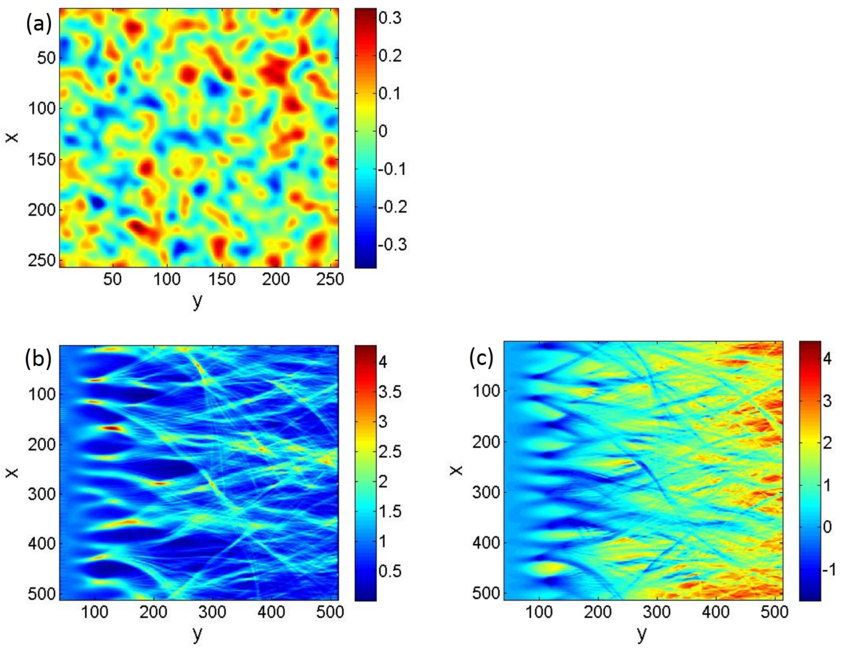
29]. A sample random potential constructed using
Gaussian bumps is shown in
Figure 1a.
The initial particles of total energy
E are distributed uniformly in the
x direction at
, with initial angles
relative to the y direction drawn from a Gaussian distribution
, with a small but finite angular spread
. (The choice of
y as the propagation coordinate is consistent with the convention adopted, for example, in Ref. [
27]). For the equations of motion (
4), the scattering strength is determined by the dimensionless quantity
in place of
. The particle trajectories will form a definite pattern of particle density for a given realization of the random potential field. Some regions (’hot spots’) will have above-average particle probability density, and others (’cold spots’) will have below-average density. Intuitively, the hot spots are more likely to be associated with local focusing of nearby particle trajectories, and the defocusing of trajectories will tend to produce cold spots.
To quantitatively monitor the degree of stretching or focusing, we define the stretching exponent
as the logarithm of the stretching ratio between nearby trajectories in the
x direction, i.e., in the direction transverse to the main flow direction
y:
where trajectories 1 and 2 are initially parallel but separated by infinitesimal
in the
x direction. The value of
describes the cumulative divergence or convergence up to time
t, and its time derivative
gives the rate of exponential divergence or convergence at time
t. The large-time limit of the stretching exponent in this 2D system is also the maximal Lyapunov exponent. While the concept of Lyapunov exponents is well established and studied in dynamical systems, the stretching exponent is employed here to study the behavior of chaotic systems for short or intermediate time scales (on scales around one Lyapunov time) and in a particular direction in phase space. For parallel ray bundles in one dimension,
coincides with the rarefaction exponent introduced by Shaw and Heller [
30]. We are interested specifically in focusing or defocusing in the transverse position coordinate, which is most relevant for fluctuations in the position space density. Quantities of this type are widely applicable, for example, in semiclassical approximations, e.g., in the Van Vleck or Gutzwiller semiclassical propagator [
32].
Very generally, dynamics in an
N-dimensional space are described by the evolution of the phase-space vector:
; and the continuous flow may be considered as the limit of a discrete-time map where the time step approaches zero. The following analysis makes use of the discrete-time picture. Consider a map
F from time step
n to the next step
,
The iteration of the tangent space is given by the Jacobian matrix:
so that the shift
in the phase vector
is mapped to the next time step
as
Therefore, the initial perturbation
evolves by a product of Jacobian matrices to
at time step
n:
where
is the monodromy or stability matrix. Similarly, in the continuous-time limit,
, the stability matrix
is given by
where
or
.
In the large-time limit, the eigenvalues of M can be written in an exponential form: , where the spectrum of Lyapunov exponents is independent of time. The matrix M has several important properties. It generates a linear, canonical transformation, and the effective dimension of the spectrum is reduced from to N, with a determinant equal to unity. Moreover, every independent constant of motion causes one pair of eigenvalues to become unity or one pair of exponents to vanish. Thus, in our 2D Hamiltonian model, with energy conserved, the eigenvalues of M are , where a single Lyapunov exponent completely captures the large-time behavior of the system.
On the other hand, the stretching exponent
defined by Equation (
6) can also be viewed as
where
, and for large time periods, the exponent
is expected to grow linearly with time:
However, the first generation of hot spots happens at intermediate time periods,
, well before the stretching exponent
begins to behave linearly. It is this intermediate behavior of
that is of greatest interest for explaining the formation mechanism of the most extreme events.
The evolution of the displacement from time
t to
can be written out explicitly as
where
,
, and
are the second derivatives of the potential field
. Then, Equation (
10) gives the monodromy matrix
M at time
t as
. For a specific trajectory, computing
requires the positions of the particle at all the time points, which can only be obtained by integrating the equations of motion. However, upon ensemble averaging over homogeneous random potentials for a given potential variance and given a two-point potential correlation function, we can consider
,
, and
to be (correlated) random numbers drawn from appropriate distributions.
Moreover, when the initial angular spread in the forward y direction is small, , the 2D model is analogous to a 1D model where the particle evolves in phase space via a time-dependent random potential line with correlation time . In the 1D model, the stretching exponent is likewise defined via the exponential divergence of two trajectories with neighboring initial positions and .
3. Results and Discussion
For numerically computing particle trajectories and stretching exponents in the 2D Hamiltonian model, we generated a Gaussian random potential
with Gaussian spatial correlations:
by Fourier convolution, as in Equation (
5), and normalized
to satisfy
and
. The choice of a Gaussian-correlated random potential was made for convenience. The above theoretical discussion does not depend on any specific choice of a random ensemble, but only on the correlation length scale
and strength
. The effect of varying the correlation function
C is addressed in detail in Ref. [
29].
The evolution was performed on a potential field of size 512 by 512 (in arbitrary units), with correlation length
and a periodic boundary condition in the transverse (
x) direction. A sample potential on a 256 by 256 grid, which was subsequently rescaled to a 512 by 512 grid for performing trajectory evolution, is shown in
Figure 1a. The specific value of
was arbitrary and served merely to set the scale for the simulation. Without loss of generality, we set
(energy). The strength of scattering
can be controlled either by varying the potential strength,
, or by controlling the angular spread,
, in the initial conditions. To avoid boundary effects, particles were launched from
inside the potential field and uniformly distributed in the transverse
x direction, with initial angles
. The initial phase-space vector for each trajectory was
, for which the initial velocity
was calculated based on its starting position
so that energy was fixed (
) for all trajectories.
Each trajectory was evolved by integrating the equations of motion, Equation (
4), using a fourth order Runge–Kutta integration method. Cubic interpolation was used for the potential
when running trajectories. The trajectories were weighted by the angular spread
, and then points along each trajectory were binned using Gaussian-shaped windows of size
to generate a ray density map
. Gaussian-shaped binning eliminates any artificial discontinuity in the binned density and effectively smooths the density data
on the scale
, which must be chosen to be small compared to the physical correlation scale
. A spacing of
in the initial trajectory positions
x, an increment of
in the initial angle
, and Gaussian intensity bins of width
with spacing 2 on the 512 by 512 grid were seen to be sufficient to achieve convergence in all the density data. Using initial positions
with spacing
and initial angles
with spacing
requires 7936 trajectories; see
Figure 1b. For stronger scattering (larger
), structures appear at a smaller scale so that the convergence of the density data requires a greater number of trajectories.
A typical density map for initial angular spread
with a potential of strength
is shown in
Figure 1b, where the first generation of caustics forms around
, and the corresponding freak index is
. Note that the particle density
is normalized to unity,
, before scattering.
Next, we demonstrate the connection between the density and the stretching exponent
. For every original trajectory launched at
, we launched a ’twin’ trajectory in the same potential at
. Then,
was computed for each trajectory according to Equation (
6); the trajectories were weighted by the initial angular spread
; and the stretching exponents were eventually mapped into the same grid that was used for density data
to produce an average position-dependent stretching rate
. Again, the binning was performed using a Gaussian window function, with a width chosen appropriately for data smoothing. Due to the long-term exponential stretching trend (Equation (
12)), the initial separation
must be chosen sufficiently small so that the separation between twin trajectories remains small during the whole time evolution. In the following, we used
. We have confirmed that our results are independent of
as long as
, where
is the correlation scale of the potential and
represents machine precision.
First, we notice the obvious connection between the density map
Figure 1b and the stretching exponent map
Figure 1c. The correlation is clearly negative; i.e., higher densities in
Figure 1b are associated with a lower stretching exponent in
Figure 1c. Indeed, every major hot spot (maximum) of the density map corresponds visually to a minimum at the same location in the stretching exponent map. This is consistent with our prediction that extreme density events would occur where the trajectories focus most significantly. Indeed, as noted above in
Section 1.2, if we assume the paraxial approximation and further assume that the density at any given point
is all coming from parallel rays originating in the neighborhood of one initial point
, then the proportionality
will hold exactly. Of course, in reality, chaotic dynamics leads at sufficient time scales to caustics and folds in the time evolution, so that the density
is given by a sum of contributions originating at different initial points with different exponents
.
In
Figure 2, we show scatter plots of the relationship between
and
before (
), during (
and
), and after (
) the region with the strongest density fluctuations. Clearly, the stretching exponent is negatively correlated with density: The strong correlation grows as the rays encounter the first generation of caustics and eventually dies off after a few Lyapunov lengths. In the region of the first caustics, extremely high densities are always associated with most negative stretching exponents, and the largest stretching exponents lead to the lowest density levels. More specifically, the particle density scales as
with constant coefficient
b around the first caustics, as seen in
Figure 2b,c. This relationship relies only on ray dynamics, and apart from the coefficient
b, it does not depend on any specific dispersion relation. At larger time scales (
), the stretching exponents
grow linearly with time, as described by Equation (
12), and the density probability distribution gradually collapses to a Gaussian one. In this regime, the correlation between the intensity and the stretching exponent declines and eventually disappears. The crossover to the large-time regime is illustrated in
Figure 2d. Nevertheless, in the regime of greatest interest, i.e., in the first caustic region
where the strongest hot spots are present, the relationship is very robust.
The distribution of the ray density is shown in
Figure 3a, where all the density data points in the region
from five realizations of the ensemble are included (while the trajectories are launched at
and the computational area extends through
, a slightly smaller region was used for collecting statistics to avoid possible edge effects). As mentioned earlier, the bulk of the distribution is close to a Gaussian distribution, whereas the fatter tail represents events of extreme densities. Then, for
Figure 3b, we averaged the stretching exponents for all the spatial cells whose density values fall within each bin in
Figure 3a. Not only in the area of the first caustics but the density distribution
and stretching exponent distribution
in general have a strong negative correlation; the locations with smaller or more negative stretching exponents are very likely to exhibit higher ray densities. Note that the fluctuations after very modest ensemble averaging in
Figure 3b are remarkably small compared to fluctuations for one realization in
Figure 2.
To further investigate the relationship between stretching exponent and ray density, we show in
Figure 4 the average and variance of these two quantities as functions of the forward distance
y. Here, for each value of
y, we collected data over all transverse positions
x and again used five different realizations of the random potential to reduce statistical noise.
The average density
increases with the factor
as required by probability conservation of the ray dynamics, where
is the angle measured from the forward
y direction. In the region of small angular spread,
, where
and
are the variances associated with the initial angular spread and the scattering, respectively. As
increases linearly with forward distance
y, the average intensity grows linearly with the forward distance, as observed in
Figure 4a.
We now turn to the stretching exponent. In the regime of small-angle scattering in the forward
y direction, we have
, and the stretching exponent
averaged over the transverse direction must grow linearly with the forward distance
y at large distances, in accordance with Equation (
12), with slope
. Furthermore, at large time scales, we can consider the process of focusing or defocusing in the transverse direction as a random walk or diffusive process, which gives rise to fluctuations in the stretching exponent
around its average value. Thus, the variance in the stretching exponents is also expected to grow linearly at large distances. The linear growth in both the average stretching exponent and its variance is observed in
Figure 4b.
Of greater interest, however, is the behavior on the scale of a Lyapunov length
, corresponding to
in
Figure 4b. The marked dip in the average exponent
at short time scales indicates substantial local focusing, which is consistent with the visual evidence in
Figure 1b. In this same region, we see in
Figure 4b strong fluctuations in the stretching exponent (as measured by the variance), and correspondingly, in
Figure 4a, large fluctuations in the ray density associated with the formation of the first and strongest hot spots. Here, we note that the density variance is closely related to the scintillation index, defined as
, and in our case,
throughout. Subsequently, the variance in the density and the scintillation index decline as the number of independent trajectories contributing to the intensity at a given point grows exponentially when
y is larger than a Lyapunov length, gradually washing out the pattern of hot spots and cold spots associated with extreme events.
The negativity of the average exponent
at short time scales is rather surprising. This unexpected behavior can be confirmed analytically using perturbation theory over a small
t, where it turns out that
scales as
, with a prefactor depending on the correlation function of the random potential [
29].
As the most significant fluctuations in both density and the stretching exponent were detected in the same spatial region, we confirm that local focusing of trajectories is directly correlated with the extreme high densities. Future work [
29] extends the scaling relationship of the form (
3) based on the scaling of the stretching-exponent statistics.


