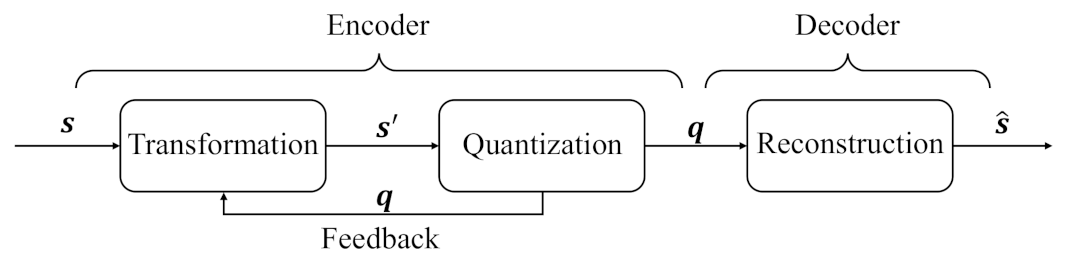
As shown in
Figure 1, a memoryless continuous sequence
of length
n is input into the transformation module, and its output is
of length
, where
m and
n are integers. Then, the continuous sequence
is quantized as a binary sequence
with the same length
. It should be noted that the quantized
is also the feedback information to transformation module. Next, the updated
seves as the output of the encoder, and it is used to reconstruct the source
.
2.1. Transformation Module
The encoder consists of the transformation and quantization modules that are detailed in
Figure 2. First, the continuous sequence
is input, and it is transformed as
, where
, and
represents the set of integer numbers from
a to
b. The sequence
is sent to the
ith quantizer
. Then, the continuous sequence
is quantized as a binary sequence
. For
, each
is fed back to the MLP of the transformation module, and
is the result. The consolidated
and
are as the input of the CNN, and the output
is as the input of
th quantizer
.
The transformation module contains the multi-layer perceptron (MLP) and the convolutional neural network (CNN). An MLP provides a nonlinear transformation to change
into
, and the quantization function
obtains the corresponding
. After that,
is returned to another MLP and transformed to
, and then it is appended on the
, which is presented as:
Then, the appended result increases one dimension of the channel, and it is sent to CNN as the input. The resulting
is as the input of
, and
is acquired.
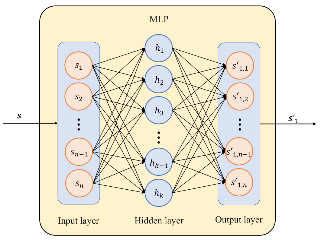
As shown in
Figure 3, the MLP is the structure of the fully-connected (FC) layer, including an input layer, an output layer and a hidden layer. The FC layer is expressed as:
where
is a small batch of inputs;
p represents the batch size; the dimensions of the input are
n;
is the output of dimension
k;
and
are the weight and bias parameters, respectively; and
indicates the set of real numbers. It should be noted that
and
refer to the input and output variables in general, respectively.
The activation functions are used to implement nonlinear transformations in the hidden layers. For the MLPs, the active function of the hidden layer is ReLU, which is shown as follows:
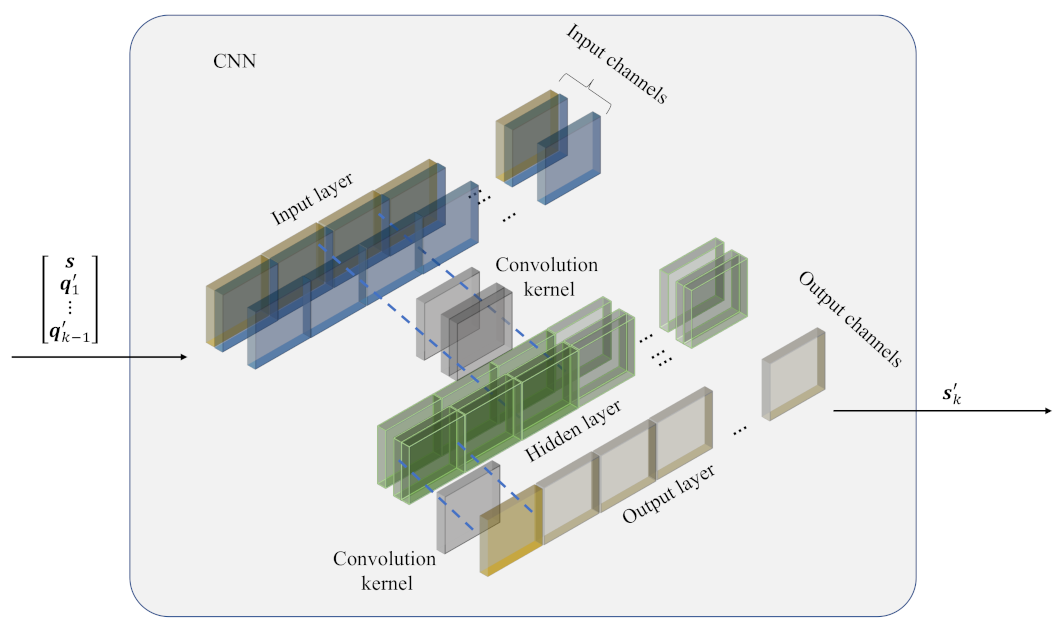
Generally, the CNN contains several convolution layers. It is commonly used in the field of computer vision with a 2D stride and kernels [
21,
22], and the 1D convolution is confronted with the sequence data [
23]. Furthermore, the convolution kernel larger than one is designed to increase the receptive field [
24,
25]. However, the memoryless continuous source has no spatial locality; hence, a larger field is unnecessary. In addition, it is convenient that the CNN in the transformation module processes multi-channel data, where the kernel size is one and the pooling layer is not needed.
Considering the aforementioned facts, the CNN only has a 1D convolutional layer with kernel size one, as shown in
Figure 4. Similarly to the MLP, the CNN has one hidden layer and uses ReLU as the active function. Actually, for each
, the convolution layer with kernel size one is calculated as:
where
is the output,
is the
ith
y in the
lth out-channel,
is the input with channel
c,
is the
ith
x in the
jth in-channel,
represents the convolution kernel,
is the
lth channel of
and
is the bias. This function can be seen as a FC layer operation in the channel dimension. Thus, in the transformation module, it is more convenient for the CNN to process the multi-channel data with fewer parameters and lower complexity than the FC layer.
2.2. Quantization
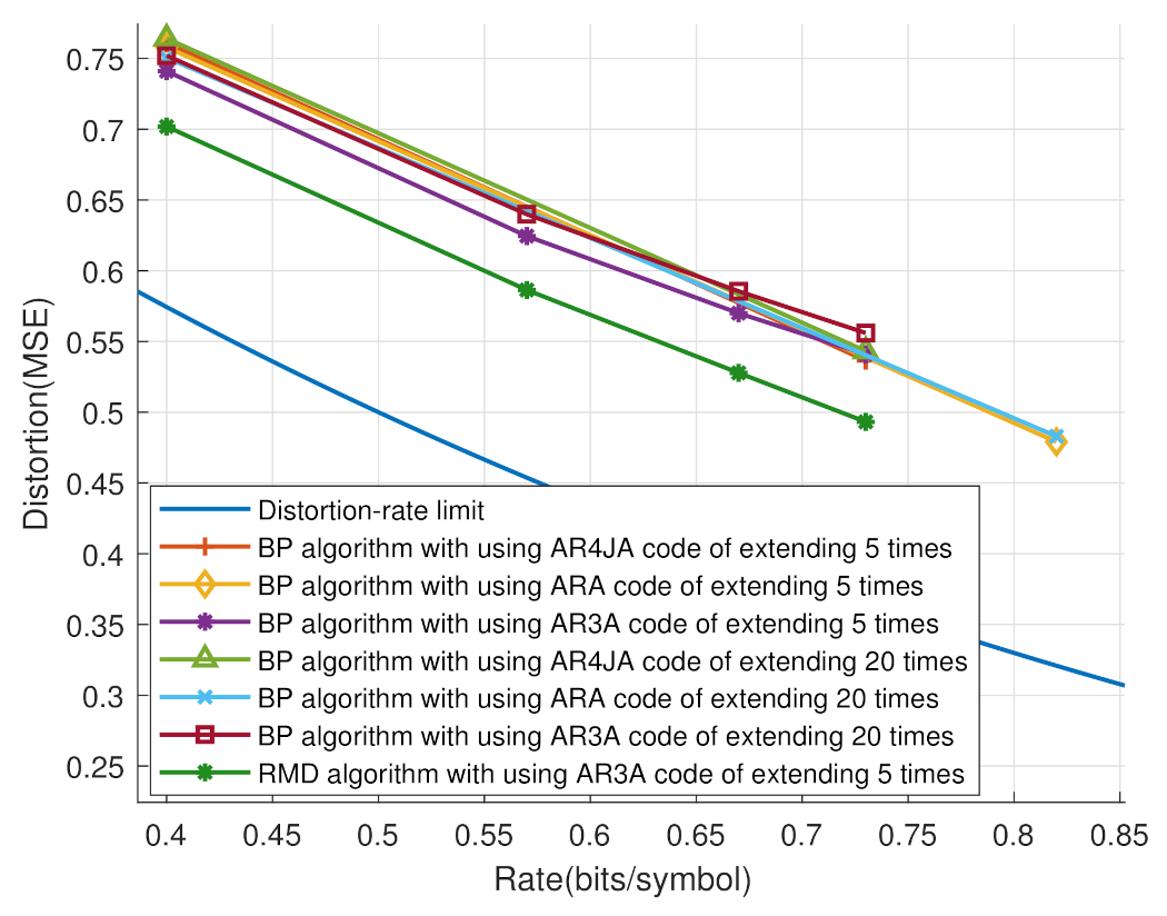
For a binary source, the BP algorithm is usually employed as the quantization for source compression. The principle of the BP quantization is based on the LDPC codebook satisfying in GF(2), where is the correct result, and the codebook is the parity check matrix of the LDPC code.
However, the continuous source is quite different from the codebook of GF(2). If the continuous sequence is directly compressed by the BP based LDPC code, it will generate a larger distortion. Hence, a new quantizer based on the RMD strategy is designed to replace the BP. The RMD strategy is described in Algorithm 1. In this condition, the compression distortion is minimized to satisfy .
Firstly, the symbols in Algorithm 1 are defined as follows:
the input source data;
iter: the maximum number of iterations;
the allocation of cost weight between variable and check nodes;
the mask vector, for which the masked nodes are set to zero;
the quantized , and also the output of the RMD algorithm;
the subscripts represent variable and check parts of symbol , respectively;
g the generation function of the LDPC code;
coe, map: the coefficients of the RMD algorithm, and map contains map and map;
fc: the cost vector of each node, and it contains fc and fc;
the sets of variable and check nodes, respectively;
the variable nodes connected with the k-th check node;
the check nodes connected with the k-th variable node;
lr: the learning rate of the training stage;
merging of two variables;
argmin the positioning function of the minimum element.
In addition, the map
function is calculated by
where
,
and
represent the
ith element of
,
and
, respectively.
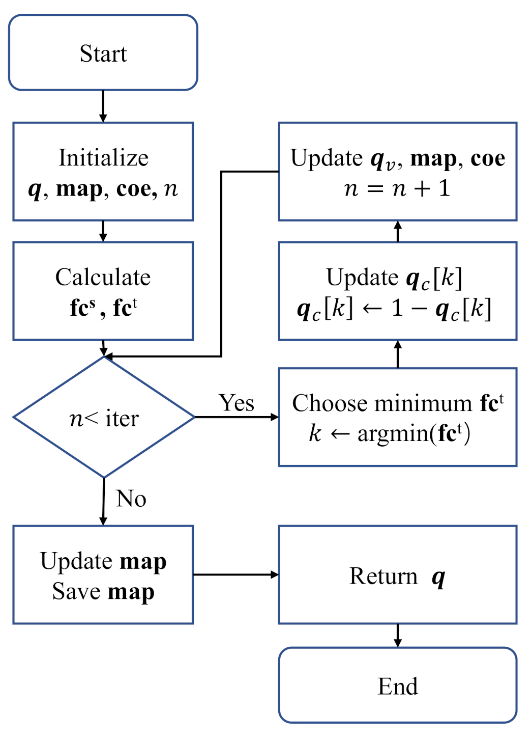
In Algorithm 1, the variables
and
are initialized from lines 1 to 6. The variable
coe is initialized according to
map and the input mask
from lines 7 to 12.
fc and
are calculated from lines 13 to 17. In the while loop,
is flipped, and it is determined by the minimum
. If
, the flipping will reduce the distortion; then,
and
need to be updated. From lines 29 to 31,
map is updated by using the gradient descent with learning rate lr, and it is saved for the next use at line 33. When the RDM algorithm is not implemented at the training stage, lines 5 and 6 will be replaced by loading
map, and lines 29 to 32 will be removed. Algorithm 2 presents the cost function of the RMD algorithm, which calculates the flip cost of each nodes and assigns them to
fc according to
coe. The flow chart of Algorithm 1 is shown in
Figure 5.
| Algorithm 1 RMD algorithm. |
| Input: |
| Output: |
| 1: |
| 2: |
| 3: |
| 4: |
| 5: map |
| 6: |
| 7: coe |
| 8: for i in do |
| 9: if then |
| 10: coe[i] |
| 11: end if |
| 12: end for |
| 13: |
| 14: fcfcfc |
| 15: for i in do |
| 16: fcfcfc |
| 17: end for |
| 18: |
| 19: while
do |
| 20: |
| 21: fc |
| 22: if then |
| 23: |
| 24: fcfc updatefcfc |
| 25: else |
| 26: break |
| 27: end if |
| 28: end while |
| 29: |
| 30: |
| 31: |
| 32: save map |
| 33: return |
| Algorithm 2 . |
| Input: |
| Output:
|
| 1: |
| 2: for i in do |
| 3: |
| 4: end for |
| 5: return
|
In the RMD algorithm, q is flipped with the minimum in each iteration satisfying . Here, the minimum indicates the maximum quantization error between itself and the associated variable node; therefore, the flipping will effectively reduce the total quantization distortion. In the training process, coe and map are updated by gradient descent. With coe and map updating, the will be calculated more accurately.
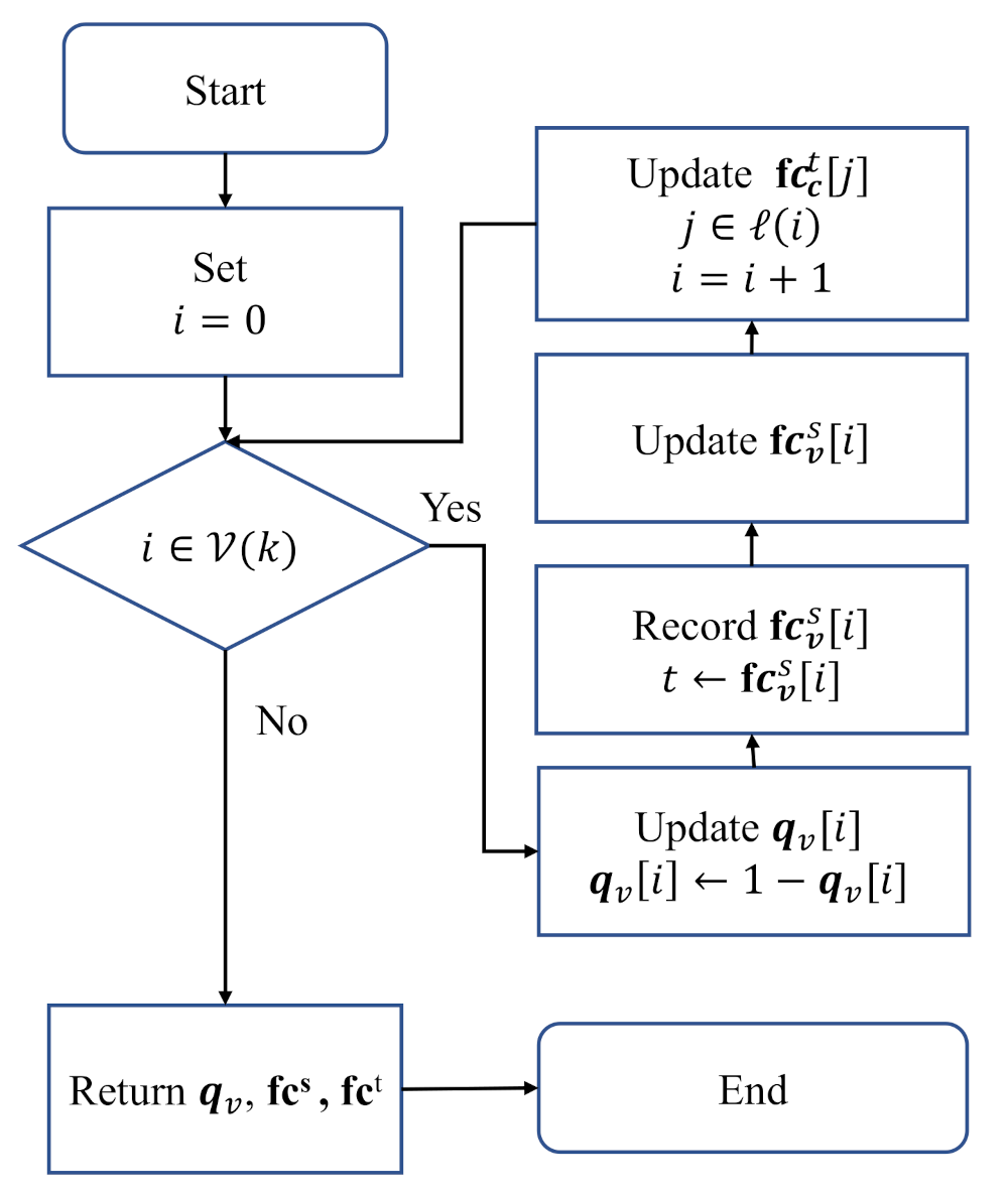
Algorithm 3 presents a quick way to update
and
. Only if
satisfying
is flipped, the corresponding
can be updated. Then, the corresponding
is refreshed by calculating
. In this case, it does not need to recalculate
and
. The flow chart of Algorithm 3 is shown in
Figure 6.
| Algorithm 3 . |
| Input: |
| Output: |
| 1: for i in do |
| 2: |
| 3: |
| 4: |
| 5: for j in do |
| 6: |
| 7: end for |
| 8: end for |
| 9: return
|
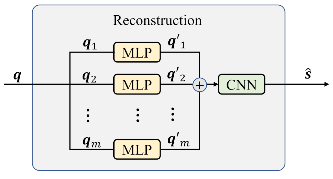
Each node i in the check matrix of the LDPC code with mask vector is filled with before the RMD training. The output is compressed as following , and it can be reconstructed by , where is the generation function of LDPC code. This allows the rate to be changed from to 1 according to the variable , where n and k are the code length and numbers of variable nodes, respectively, and represents the number of element 1 in mask vector .
The computational complexity of the proposed RMD algorithm is
where
n is the number of check nodes;
t is the number of iterations satisfying
; and
and
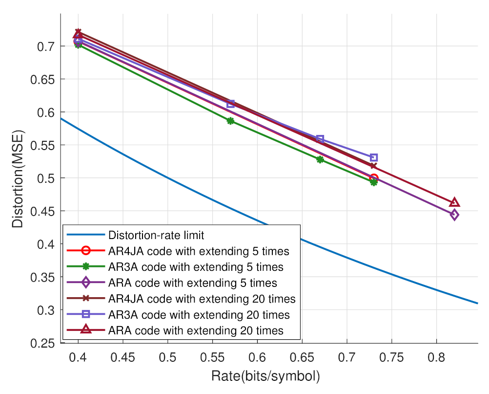
are the degrees of the variable and check nodes, respectively. In addition, the number of iterations is limited to 30 in the RMD algorithm, and the BP algorithm needs over 100 iterations. Overall, the computational and time complexities of the RMD algorithm are both lower than those of the BP algorithm.


