1. Introduction
Compared with classical separate source and channel coding schemes, a common objective of joint source-channel coding (JSCC) schemes is to make full use of the source and channel information in order to boost the performance of the overall system. As a promising coding structure, a JSCC scheme consisting of two low-density parity-check (LDPC) codes was proposed in [
1], where an LDPC code is for source compression and the other one is for channel coding. This scheme is referred to as the double LDPC (D-LDPC) coding system. Further, various LDPC codes have been investigated for D-LDPC systems, such as protograph LDPC codes [
2,
3], quasi-cyclic LDPC codes [
4] and spatially coupled LDPC codes [
5].
In the D-LDPC coding system, a core idea is the introduction of a linking matrix setting up the connections between the check nodes (CNs) of the source LDPC code and the variable nodes (VNs) of the channel LDPC code, and we name it as the source check–channel variable (SC-CV) linking matrix. Using the SC-CV linking matrix, the joint belief propagation (BP) decoding can iteratively exchange the source redundancy and channel state information to improve the system performance. To achieve a better performance, the non-zero column vectors in the linking matrix should connect to the VNs with larger degrees in the channel LDPC code [
6]. Moreover, the linking matrix can be optimized considering the degree distribution of the check nodes (CNs) of the source LDPC code [
7].
In this paper, a generalized SC-CV linking matrix is introduced into the D-LDPC coding system. The conventional SC-CV linking matrix consists of a zero matrix and an identity matrix, i.e., both the row and column weights being 1, which implies a one-to-one mapping between the source coding and channel coding. However, this mapping may not take full advantage of the source redundancy and channel state information. Therefore, a more general linking matrix is introduced for the purpose of providing more connections between the CNs of the source LDPC code and the VNs of the channel LDPC. Consequently, the identity matrix in the SC-CV linking matrix will be replaced by a non-identity matrix. Note that the identity matrix [
6], including its row and column switching [
7], becomes a special case of the proposed general linking matrix.
1.1. Related Work of D-LDPC Code Systems
In recent years, a majority of the work for D-LDPC code systems has been studied in order to improve the bit error rate (BER) performance in the water-fall region and error-floor region. The former is evaluated by the channel decoding threshold and the latter is evaluated by the source decoding threshold. For DP-LDPC code systems, a joint protograph extrinsic information transfer (JPEXIT) algorithm [
8] was proposed to analyze the channel decoding threshold. Based on the JPEXIT algorithm, an important structure, i.e., a degree-2 VN, was analyzed for DP-LDPC codes [
9]. Several optimized channel protographs with more degree-2 VNs were proposed to lower the channel decoding threshold [
10,
11]. Moreover, this degree-2 VN structure can also help improve the source decoding threshold, which is analyzed by the source PEXIT (SPEXIT) algorithm [
12]. In order to improve the error-floor performance, a linking matrix connecting the VNs of the source LDPC code and the CNs of the channel LDPC code, denoted as the source variable–channel check (SV-CC) linking matrix, was introduced in [
6]. Further, several SV-CC linking matrices combined with source protographs are optimized based on the generalized SPEXIT algorithm [
13]. Some integrated design work [
14,
15,
16] of the joint protograph were conducted by differential evolution [
17], where the cost function is the calculation of the decoding threshold. In addition, the improved sliding window decoding algorithm [
18] and the joint grouping shuffled scheduling decoding algorithm [
19] were proposed for the D-LDPC codes system.
1.2. Contribution
However, the aforementioned D-LDPC code systems are all based on the identity SC-CV linking matrix. The introduction of the non-identity linking matrix enables a more effective decoding information (e.g., source redundancy and channel state information) transfer between the source and channel LDPC codes.
The novelty and contributions of this paper can be summarized as follows.
- (1)
A general SC-CV linking matrix is introduced into the D-LDPC code system and the corresponding encoding and decoding algorithms are generalized.
- (2)
In order to analyze the impacts of the general SC-CV linking matrix on both the channel decoding threshold and source decoding threshold, the corresponding EXIT algorithm is proposed.
- (3)
Given several pairs of source and channel protographs, some general linking matrices constructed by a matrix operation are optimized.
1.3. Paper Organization
The remainder of this paper is organized as follows.
Section 2 presents the preliminaries of the conventional D-LDPC code system. In
Section 3, the novel D-LDPC code system with the proposed general linking matrix is presented as well as the generalized encoding and decoding algorithms. In
Section 4, the evaluation of the source and channel decoding thresholds is described based on the JPEXIT algorithm. The structure of the proposed general linking matrix is first analyzed in
Section 5, and then several general linking matrices are optimized for the given source and channel protographs pairs. The simulation results and comparisons are discussed in
Section 6, and finally,
Section 7 draws a conclusion of this paper.
2. Preliminaries on Conventional D-LDPC Coding Systems
An LDPC code can be represented by the sets , respectively, indicating the set of VNs, CNs and the edges between VNs and CNs. It can also be represented by a parity-check matrix , where or 1, indicating if there is a connection from the j-th VN to the i-th CN.
Consequently, a JSCC system based on D-LDPC codes can be represented by the following parity-check matrix
,
where
(size ) is the parity-check matrix of the source LDPC code;
(size ) is the parity-check matrix of the channel LDPC code;
of dimension is the source check–channel variable (SC-CV) linking matrix, indicating the connections between CNs of and VNs of .
of dimension is the source variable–channel check (SV-CC) linking matrix, indicating the connections between VNs of and CNs of .
Remark 1. The non-zerolowers error floors but increases channel decoding thresholds for a given code pairand.
For simplicity, the caseis considered in this paper. As all that really matters is the part,
the linking matrix only denotes thein the following content unless otherwise stated. Thus, the joint parity-check matrixis changed to be In the conventional D-LDPC coding system, consists of an identity matrix, i.e., (size ), and an all zero matrix. The identity matrix specifies the one-to-one connection between the CNs of and the VNs of . A generator matrix with a systematic form is obtained from by Gaussian elimination.
2.1. Encoding
For an independent and identically distributed (i.i.d.) Bernoulli (
) source, an original source sequence
(
) is encoded into codeword
by a parity-check matrix
, i.e.,
where
of dimension
denotes the compressed source bit sequence, and
represents matrix transpose operation. Next, the compressed bits
is encoded by the matrix
, i.e.,
where
is a parity bit sequence
(size
). Some bits in
will be punctured if a punctured LDPC code
is utilized. The left bits in
are modulated by binary phase-shift keying (BPSK) and sent over an additive white Gaussian noise (AWGN) channel with noise following Gaussian distribution
, where
(
is the average energy of each channel bit and
is the average energy of channel noise). The overall channel coding rate is expressed as
where
is the length of punctured bits.
2.2. Decoding
Let us first define
(
) and
(
). At the receiver, the corresponding initial log-likelihood ratio (LLR) of
is calculated by
for the transmitted part and 0 for the punctured part, where
is the received signal. We assume that the source statistics are known by the receiver (the source statistics can also be estimated during decoding procedure), and the LLR of sequence
is evaluated by
. Note that the parity-check matrix
in (
2) can be regarded as a single LDPC code, by globally viewing the CNs and VNs of each component matrix. Accordingly, the joint decoding algorithm based on belief propagation (BP) can be performed on a single
, as described below.
Let
(respectively,
) be the information passed from the
j-th VN (respectively,
i-th CN) to
i-th CN (respectively,
j-th VN) at the
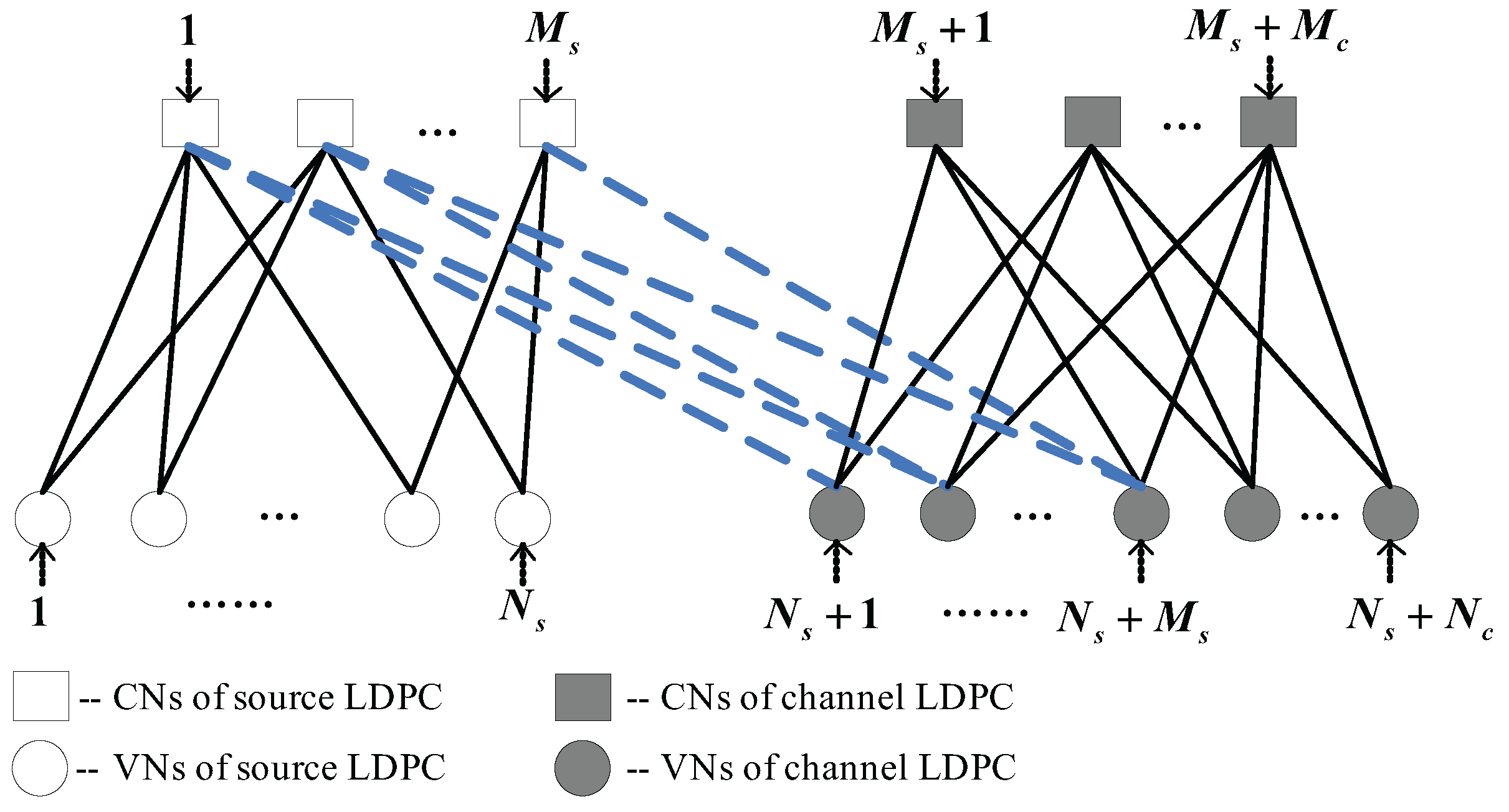
k-th iteration. As shown in
Figure 1, the corresponding iterative decoding procedure is described as follows.
3. The Proposed D-LDPC Code System with a General Linking Matrix
Different from the separated source LDPC coding and channel LDPC coding systems, the conventional D-LDPC code system sets up its connections via , which is a simple identity matrix from the perspective of encoding. As for the functionality of from a decoding perspective, the information from channel decoding can be passed to source decoding, and vice versa, which allows to exchange the source redundancy and channel state information and accelerate the decoding process.
However, the one-to-one connection defined by may not make full use of this decoding information. Thus, a general linking matrix, i.e., non-identity matrix , denoted as , will be introduced. The generalized encoding and decoding algorithm with a general linking matrix will be described as follows.
3.1. Generalized Encoding
The source coding procedure can be re-written as follows. A generated matrix with a systematic form
should first be obtained from
by Gaussian elimination (denoted as “→”), i.e.,
As
is an identity matrix,
can correspond to
and
.
Thus, in order to obtain the compressed bits
, the encoding can be calculated by
where the calculation of
is the (
3).
When
, the
should be first transformed into the systematic form, i.e.,
The corresponding generated matrix
and
Taking the channel coding procedure (
4) into consideration, the total encoding algorithm can be generalized by
3.2. Generalized Decoding
By doing so, the overall joint parity-check matrix
can be expressed as
Considering that the vector
satisfies
the joint decoding procedure from (
6) to (
11) can be directly applied to the proposed D-LDPC coding system and the (
12) should be adjusted as
where the joint Tanner graph of the proposed system is illustrated in
Figure 2.
4. EXIT Analysis for the Joint Protograph with a General Linking Matrix
4.1. Joint Protograph
In order to illustrate the advantages of the application of the general linking matrix in the D-LDPC code system, the structured protograph LDPC codes are considered here. Different from the degree distribution representation of an irregular LDPC code, a protograph LDPC code is defined by a small protomatrix
(
is a non-negative integer), and a practical large parity-check matrix can be obtained by a “copy-and-permute” operation, such as the well-known progressive edge growth (PEG) algorithm [
20]. The protomatrix not only clearly observes the change in code structure but also directly indicates the performance of the corresponding large parity-check matrix. Therefore, we only need to focus on the design of the small protomatrix of the corresponding large general linking matrix.
The joint protomatrix of a double protograph LDPC (DP-LDPC) code system is represented by
where
(size ) is the protomatrix of the source protograph LDPC code;
(size ) is the protomatrix of the channel protograph LDPC code;
(size ) is the protomatrix associated with the SC-CV linking matrix;
of dimension (note that ) is the protomatrix of the general linking matrix and is an identity protomatrix, both of them corresponding to ;
If a punctured protograph is used, then we denote by the number of punctured VNs.
In order to obtain the corresponding parity-check matrix , the PEG algorithm with a parameter is employed to remove all parallel edges at the first step. Next, the same PEG algorithm with parameter is performed again to obtain a parity-check matrix of desired sizes.
4.2. Joint Protograph EXIT Algorithm
In the D-LDPC coding system, two decoding thresholds should be considered, i.e., channel decoding threshold and source decoding threshold . The channel decoding threshold reflects the ultimate performance in the water-fall region. On the other hand, the source decoding threshold indicates the performance of the error-floor level, and a higher implies a lower error-floor level.
In order to determine the channel and source decoding thresholds, the JPEXIT algorithm has to be described. Let us first define the following five types of mutual information (MI).
: the extrinsic MI from j-th VN to i-th CN;
: the extrinsic MI from i-th CN to j-th VN;
: the a prior MI from j-th VN to i-th CN;
: the a prior MI from i-th CN to j-th VN;
: the MI between a posterior LLR evaluated by j-th VN and the corresponding bit .
In addition, two functions
and
are defined.
represents the MI between a binary bit sent over an AWGN channel and its corresponding LLR value, and it is given by
Moreover,
is a manipulation of the function
, for a binary source with an i.i.d. Bernoulli distribution (
). In other words, the equivalent channel is a binary symmetric channel with
, and it is defined as
where
is the MI between the VN of the source and
,
and
.
Furthermore, the update procedure of the MI can be summarized as follows.
For
and
, if
,
For
and
, if
,
where
If , .
For
and
,
For
and
, if
,
where
Note that
is the inverse function of
, and if
,
.
For
and
,
where
The above MI update procedure will be conducted iteratively until all
or the preset total number
of iterations is reached. We point out that
for all
, implies that the decoding performance has converged.
In summary, the
can be viewed as a function of independent variables
,
,
and
, i.e.,
where
can be calculated from
. To this end, for a given
and
, the channel decoding threshold
is the minimum value
, making all
[
10].
4.3. Evaluation of the Decoding Threshold
The channel decoding threshold
indicates the performance of the water-fall regime. The conventional JPEXIT analysis only focuses on the protomatrix
with an identity
. Because a more general linking protomatrix
is introduced, the MI transfer in
will be changed and thus the channel decoding threshold will be different. Note that the MI updates from (
25) to (
29) will still remain the same.
The source decoding threshold
indicates the performance of the error-floor level, which is the lowest BER when
approaches infinity. For the calculation of
in the conventional source protograph EXIT (SPEXIT) analysis [
12,
13], it is assumed that the MI transfer from the channel part (
) to the source part (
) is full. Here, we set the
for
to make the information from the channel be fully correct. Thus, the source decoding threshold will not be affected by the structure of
as well as
and is decided by the structure of the source protomatrix
.
In all, introducing the general linking matrix will only affect the channel decoding threshold of the DP-LDPC coding system.
5. Design of General Linking Matrices
5.1. Structure of the General Linking Protomatrix
In order to efficiently optimize the general linking matrix, we should first discuss its structure. should be a non-singular matrix in order to keep the matrix rank of the same as that of , which also keeps the length of the compressed bit .
Therefore, the general linking protomatrix is also a non-singular matrix. From the matrix theory, the elementary row transformation is defined by three kinds of matrix operations as follows:
Multiply a non-zero value to one row of the matrix;
Add a multiple of one row in the matrix to another row;
Change the position of two rows in the matrix.
The elementary column transformation can also be defined via replacing the “row” with “column” in the definition above. Motivated by this, a non-singular square protomatrix (e.g.,
) can be obtained by performing a series of elementary operations on an identity matrix (e.g.,
). It is worth pointing out that if only operation-3 is performed for an identity matrix
, it corresponds to the optimization of the connections between the VNs of the source protograph and the CNs of the channel protograph [
7].
In order to further illustrate the structures of the general linking protomatrix, we take the following joint protomatrix as an example, i.e.,
where the linking part is a
identity matrix. The joint protograph is shown in
Figure 3a. If operation-3 of the elementary transformation is performed, the joint protograph could be changed to
Figure 3b, which is denoted by
. Similarly, the protomatrix
shown in
Figure 3c could be obtained by the operation-1, and
demonstrated in
Figure 3d could be obtained by the combination of the operation-1 and operation-2. The protomatrix
is given by
5.2. Optimization Method
As mentioned above, the protomatrix
can be constructed from the elementary matrix operations, which also determines the complexity (the row or column weight of the matrix can measure the complexity). In other words, if a set
consisting of all possible element values is given, the complexity of designing
is determined. The complexity of the optimization also relies on the size of protomatrix, i.e.,
. If the general linking protomatrix is optimized directly, we should design a specific structure and simultaneously optimize the connections between the CNs of source protomatrix and the VNs of channel protomatrix. In [
11], it is indicated that
should connect to the VNs with the largest degree in the
for the optimal channel decoding threshold. Therefore, the procedures of optimizing general linking protomatrix can be summarized in three steps:
Select an appropriate and ;
Determine the connecting VNs of the channel protomatrix by employing the identity protomatrix ;
Design the specific structure of (including the connecting CNs of the source protomatrix) based on the matrix operations of elementary row/column transformation.
5.3. Optimization Examples
The main tested parameters in the optimization are shown in
Table 1.
Example 1. We start from a joint protomatrix optimized in [9], i.e.,where is the R4JA code, is the re-designed IAR4JA code [9] and is assumed to connect the VNs of and in the . The source decoding threshold shown in Table 2 is 0.028 and the channel decoding threshold at and is −3.441 dB and −1.357 dB, respectively. For moderate searching complexity, the Θ here is set to be . All possible are analyzed by calculating channel and source decoding thresholds. Several representative are considered and their corresponding joint protomatrices are given in Table 2, where has the smallest and is a counterpart example. All of them have the same and . By comparing , and , it is found that the source decoding threshold has little difference, but the channel decoding threshold of is 0.582 dB, which is 2.084 dB lower than that of and for source statistic . This difference is 0.321 dB, which is 1.027 dB for source statistic .
Example 2. Another joint protomatrix with a larger size at source statistic is taken as an example. The joint protomatrix includes a rate-1/2 source protograph and a rate-1/2 channel protograph given in [12]. In addition, we select and . According to step-(2), the is given byand it has a channel decoding threshold of −1.666 dB. Next, the specific structure of general linking protomatrix is optimized as The corresponding joint protograph is denoted by , which has a channel decoding threshold of −2.605 dB.
In the case of
, the optimized general linking protomatrix
is the same as that in the case of
, and we denote by
the corresponding protomatrix, with
dB. The optimized general linking protomatrix
is given by
and the corresponding joint protograph is denoted by
, which has a channel decoding threshold of −1.149 dB. It is worth mentioning that the optimal
is different for the case of
and
, although they have the same
and
.
By observing the optimized general linking matrix, it is found that the VN with the largest degree is located in the same column as the VN with the largest degree of the channel protomatrix. Although this is not derived by mathematical proof, such experience can reduce the search complexity of the optimization.
6. Simulation and Comparison Results
The BER simulation is carried out to verify the analysis of the JPEXIT algorithm. The BER simulation is performed over AWGN channels and the maximum iteration number of the joint BP decoding algorithm is set to 100.
6.1. The BER Simulation of Example 1
The effect of introducing the general linking protomatrix
for the water-fall region and error-floor region is analyzed in this subsection. Firstly, the two-step PEG algorithm mentioned in
Section 4 with parameters
and
is performed for
,
and
, and the corresponding parity-check matrices are
,
and
, respectively. Consequently, the code length is
. The channel coderate
R is 1/2.
Figure 4 shows the BER performance when
and
. For the case of
, the
outperforms
and
by 1.57 dB and 0.37 dB at BER =
, respectively. In the case of
, the coding gain in the water-fall region remains the same as the case of
, and they show an error floor at a BER =
, which is almost the same level. All of the BER simulation is in line with the source and channel.
Therefore, it can be concluded that the introduction of the general linking matrix plays an important role in the water-fall region, but it has limited effect on the error-floor region.
6.2. The BER Simulation of Example 2
The superiority of optimizing the general linking matrix is further discussed in this subsection. For a target size of , the two-step PEG algorithm with and is performed for , , and , and the corresponding parity-check matrices are , , and , respectively.
Figure 5 shows the BER performance for
and
. In the case of
, the BER performance of
achieves a 0.62 dB coding gain over
at a BER =
. The BER performance improvement between
and
is only 0.36 dB for the case of
. It can be concluded that the coding gain of optimizing
becomes small with an increasing source entropy for the same pair of the source protograph and channel protograph. The same phenomenon appears in
Figure 4 for the comparison between
and
.
6.3. Complexity Comparisons
In the BP decoding, the update in the CNs dominates the total complexity, which is represented by the average degree
of a joint protograph, shown in
Table 3. The decoding complexity of the proposed joint protograph increases by
compared with the conventional ones, which stays in a comparable complexity level.
7. Conclusions
In conventional D-LDPC code systems, an identity linking matrix sets up the one-to-one connection between the source coding and channel coding, but this connection can not take full advantage of the decoding information. In this paper, a general linking matrix providing more connections is introduced into the D-LDPC code system to generalize the joint encoding procedure. Moreover, protograph LDPC codes are taken as examples for demonstrating the strengths of the proposed general linking matrices. By the aid of the JPEXIT algorithm, several general linking protomatrices to improve the channel decoding threshold are optimized. The simulation results are in line with the JPEXIT analysis, and the coding gain of the proposed DP-LDPC is 0.36–1.57 dB, which verify the superiority of the D-LDPC coding system with the proposed linking matrix.
It should be pointed out that the proposed optimization of the general linking matrix and DP-LDPC code system can also be applicable to other types of LDPC codes. The optimization of the general linking matrices over the other scenario, e.g., the joint shuffled scheduling decoding [
19], the Gaussian multiple access channel [
21], the non-linear modulation [
22] and the non-standard coding channel [
23] (e.g., optical communication [
24] and an on-body channel [
25]), can be studied in future work.
Author Contributions
Conceptualization, Q.C. and H.W.; methodology, Q.C. and G.C.; software, Q.C.; validation, Z.X., Q.C. and H.W.; formal analysis, Q.C. and H.W.; investigation, Q.C. and H.W.; resources, Q.C.; data curation, Q.C.; writing—original draft preparation, Q.C.; writing—review and editing, H.W. and G.C.; visualization, Z.X.; supervision, Z.X.; project administration, Q.C. and G.C.; funding acquisition, Q.C. and G.C. All authors have read and agreed to the published version of the manuscript.
Funding
This work was supported in part by the National Natural Science Foundation of China under Grants 62101195 and 62071129, the Science Foundation of the Fujian Province, China (Grant No. 2020J05056), the Fujian Province Young and Middle-aged Teacher Education Research Project (No. JAT220182), the Jimei University Startup Research Project (No. ZQ2022039), the Fundamental Research Funds for the Central Universities (ZQN-1008) and the Scientific Research Funds of Huaqiao University (20BS105) and the Scientific Research Foundation of Jimei University (No. XJ2022000201).
Institutional Review Board Statement
Not applicable.
Informed Consent Statement
Not applicable.
Data Availability Statement
Not applicable.
Conflicts of Interest
The authors declare no conflict of interest.
Abbreviations
The following abbreviations are used in this manuscript:
| AWGN | additive white Gaussian noise |
| APP | a posteriori probability |
| BER | bit error rate |
| BP | belief propagation |
| BPSK | binary phase-shift keying |
| CNs | check nodes |
| D-LDPC | double low-density parity check |
| EXIT | extrinsic information transfer |
| JEXIT | joint extrinsic information transfer |
| JPEXIT | joint protograph EXIT |
| JSCC | joint source-channel coding |
| LLR | log-likelihood ratio |
| MI | mutual information |
| PEG | progressive edge growth |
| SC-CV | source check–channel variable |
| SPEXIT | source protograph EXIT |
| SV-CC | source variable–channel check |
| VNs | variable nodes |
References
- Fresia, M.; Perez-cruz, F.; Poor, H.V.; Verdu, S. Joint source and channel coding. IEEE Signal Process. Mag. 2010, 6, 104–113. [Google Scholar] [CrossRef]
- He, J.; Wang, L.; Chen, P. A joint source and channel coding scheme based on simple protograph structured codes. In Proceedings of the Symposium on Communications and Information Technologies, Sydney, Australia, 2–5 October 2012; pp. 65–69. [Google Scholar]
- Chen, Q.; He, Y.; Chen, C.; Zhou, L. Optimization of protograph LDPC codes via surrogate channel for unequal power allocation. IEEE Trans. Commun. 2023. early access. [Google Scholar] [CrossRef]
- Lin, H.; Lin, S.; Abdel-Ghaffar, K. Integrated code design for a joint source and channel LDPC coding scheme. In Proceedings of the IEEE Information Theory and Applications Workshop (ITA), San Diego, CA, USA, 12–17 February 2017; pp. 1–9. [Google Scholar]
- Golmohammadi, A.; Mitchell, D.G.M. Concatenated spatially coupled LDPC codes with sliding window decoding for joint source-channel coding. IEEE Trans. Commun. 2022, 2, 851–864. [Google Scholar] [CrossRef]
- Neto, H.; Henkel, W. Multi-edge optimization of low-density parity-check codes of joint source-channel coding. In Proceedings of the IEEE Systems, Commun. and Coding (SCC), Munich, Germany, 21–24 January 2013; pp. 1–6. [Google Scholar]
- Liu, S.; Chen, C.; Wang, L.; Hong, S. Edge connection optimization for JSCC system based on DP-LDPC codes. IEEE Wirel. Commun. Lett. 2019, 4, 996–999. [Google Scholar] [CrossRef]
- Wu, H.; Wang, L.; Hong, S.; He, J. Performance of joint source channel coding based on protograph LDPC codes over Rayleigh fading channels. IEEE Commun. Lett. 2014, 4, 652–655. [Google Scholar] [CrossRef]
- Chen, Q.; Wang, L.; Hong, S.; Xiong, Z. Performance improvement of JSCC scheme through redesigning channel codes. IEEE Commun. Lett. 2016, 6, 1088–1091. [Google Scholar] [CrossRef]
- Chen, Q.; Wang, L.; Hong, S.; Chen, Y. Integrated design of JSCC scheme based on double protograph LDPC codes system. IEEE Commun. Lett. 2019, 2, 218–221. [Google Scholar] [CrossRef]
- Hong, S.; Chen, Q.; Wang, L. Performance analysis and optimization for edge connection of JSCC scheme based on double protograph LDPC codes. IET Commun. 2018, 2, 214–219. [Google Scholar] [CrossRef]
- Chen, C.; Wang, L.; Liu, S. The design of protograph LDPC codes as source code in a JSCC system. IEEE Commun. Lett. 2018, 4, 672–675. [Google Scholar] [CrossRef]
- Chen, Q.; Lau, F.C.M.; Wu, H.; Chen, C. Analysis and improvement of error-floor performance for JSCC Scheme based on double protograph LDPC codes. IEEE Trans. Vehi. Tech. 2020, 12, 14316–14329. [Google Scholar] [CrossRef]
- Chen, C.; Wang, L.; Lau, F. Joint optimization of protograph LDPC code pair for joint source and channel coding. IEEE Trans. Commum. 2018, 8, 3255–3267. [Google Scholar]
- Liu, S.; Wang, L.; Chen, J.; Hong, S. Joint component design for the JSCC system based on DP-LDPC codes. IEEE Trans. Commum. 2020, 9, 5808–5818. [Google Scholar] [CrossRef]
- Xu, Z.; Wang, L.; Hong, S.; Chen, G. Design of code pair for protograph-LDPC codes-based JSCC system with joint shuffled scheduling decoding algorithm. IEEE Commun. Lett. 2021, 12, 3770–3774. [Google Scholar] [CrossRef]
- Das, S.; Suganthan, P.N. Differential evolution: A survey of the state-of-the-art. IEEE Trans. Evol. Comput. 2011, 1, 4–31. [Google Scholar] [CrossRef]
- Lian, Q.; Chen, Q.; Zhou, L.; He, Y.; Xie, X. Adaptive decoding algorithm with variable sliding window for double SC-LDPC coding system. IEEE Commun. Lett. 2023, 2, 404–408. [Google Scholar] [CrossRef]
- Chen, Q.; Ren, Y.; Zhou, L.; Chen, C.; Liu, S. Design and analysis of joint group shuffled scheduling decoding algorithm for double LDPC codes system. Entropy 2023, 25, 357. [Google Scholar] [CrossRef]
- Hu, X.-Y.; Eleftheriou, E.; Arnold, D.M. Regular and irregular progressive edge-growth Tanner graphs. IEEE Trans. Info. Theory 2005, 1, 386–398. [Google Scholar] [CrossRef]
- Chen, P.; Shi, L.; Fang, Y.; Lau, F.C.M.; Cheng, J. Rate-diverse multiple access over Gaussian channels. IEEE Trans. Wire. Commun. 2022. early access. [Google Scholar] [CrossRef]
- Fang, Y.; Zhuo, J.; Ma, H.; Mumtaz, S.; Li, Y. Design and analysis of a new index-modulation-aided DCSK system with frequency-and-time resources. IEEE Trans. Vehi. Tech. 2023. early access. [Google Scholar] [CrossRef]
- Chen, Q.; Wang, L. Design and analysis of joint source channel coding schemes over non-standard coding channels. IEEE Trans. Vehi. Tech. 2020, 8, 5369–5380. [Google Scholar] [CrossRef]
- Zheng, Z.; Yang, C.; Yang, C.; Wang, Z. Energy consumption modeling and analysis for short-reach optical transmissions using irregular LDPC codes. Optics Express 2022, 24, 43852–43871. [Google Scholar] [CrossRef]
- Song, D.; Ren, J.; Wang, L.; Chen, G. Designing a common DP-LDPC codes pair for variable on-body channels. IEEE Trans. Wire. Commun. 2022, 11, 9596–9609. [Google Scholar] [CrossRef]
| Disclaimer/Publisher’s Note: The statements, opinions and data contained in all publications are solely those of the individual author(s) and contributor(s) and not of MDPI and/or the editor(s). MDPI and/or the editor(s) disclaim responsibility for any injury to people or property resulting from any ideas, methods, instructions or products referred to in the content. |
© 2023 by the authors. Licensee MDPI, Basel, Switzerland. This article is an open access article distributed under the terms and conditions of the Creative Commons Attribution (CC BY) license (https://creativecommons.org/licenses/by/4.0/).


