
DUS Topp–Leone-G Family of Distributions: Baseline Extension, Properties, Estimation, Simulation and Useful Applications

 , and
, and 
Abstract
1. Introduction
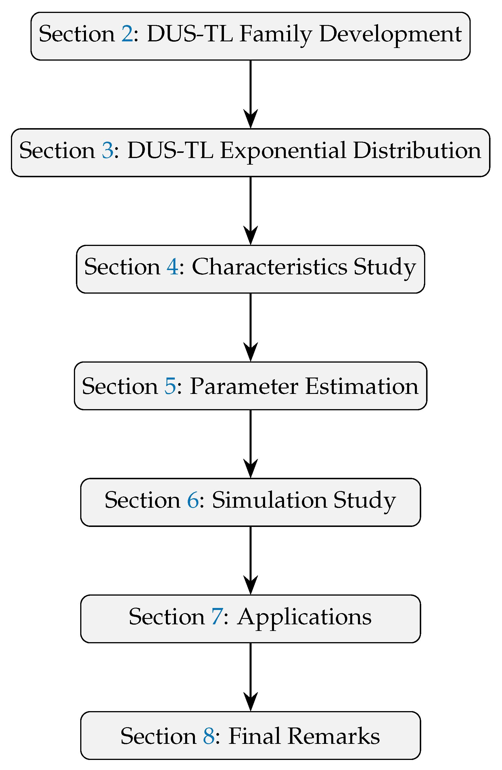
2. The DUS Topp–Leone Family of Distributions
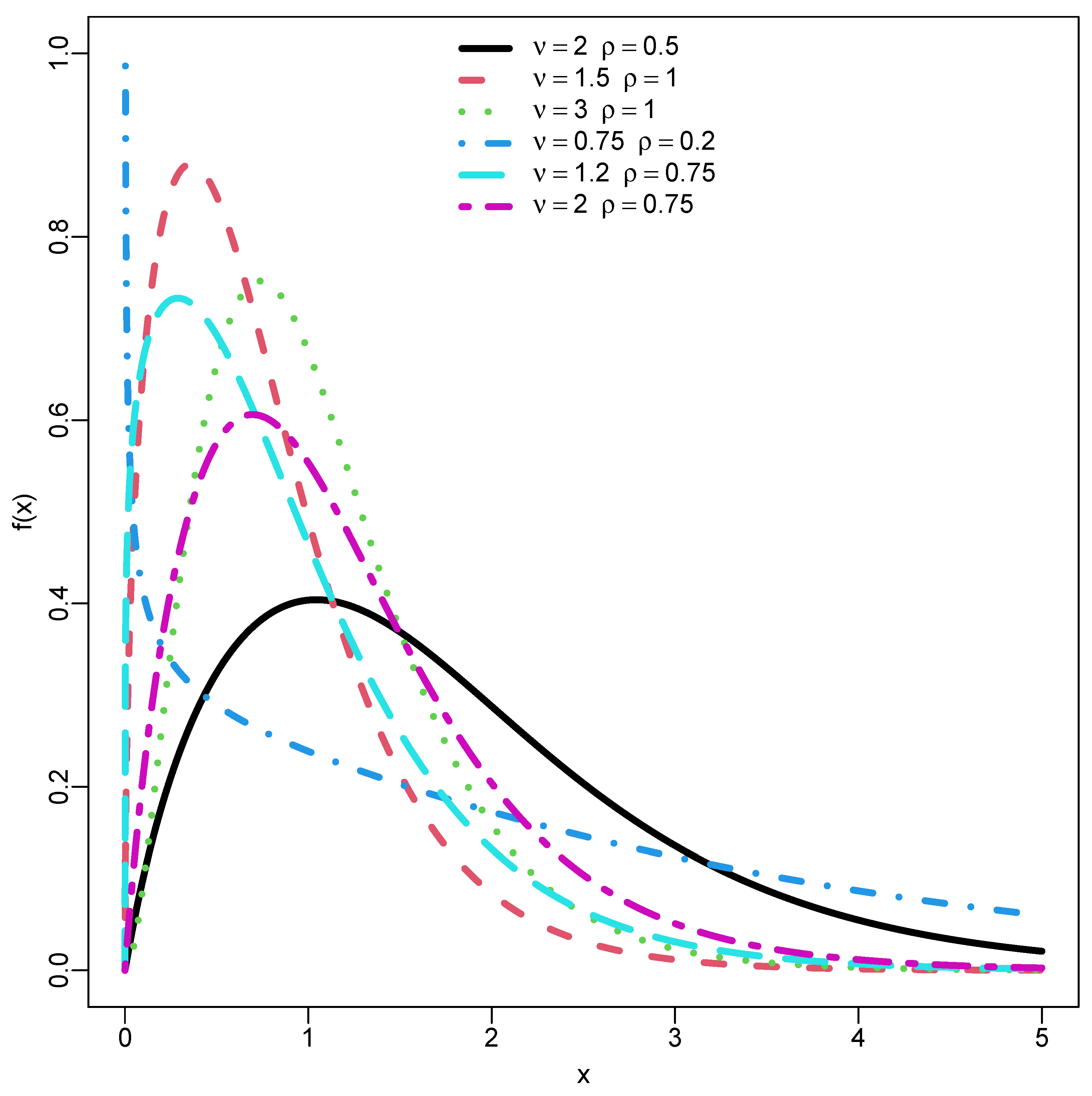
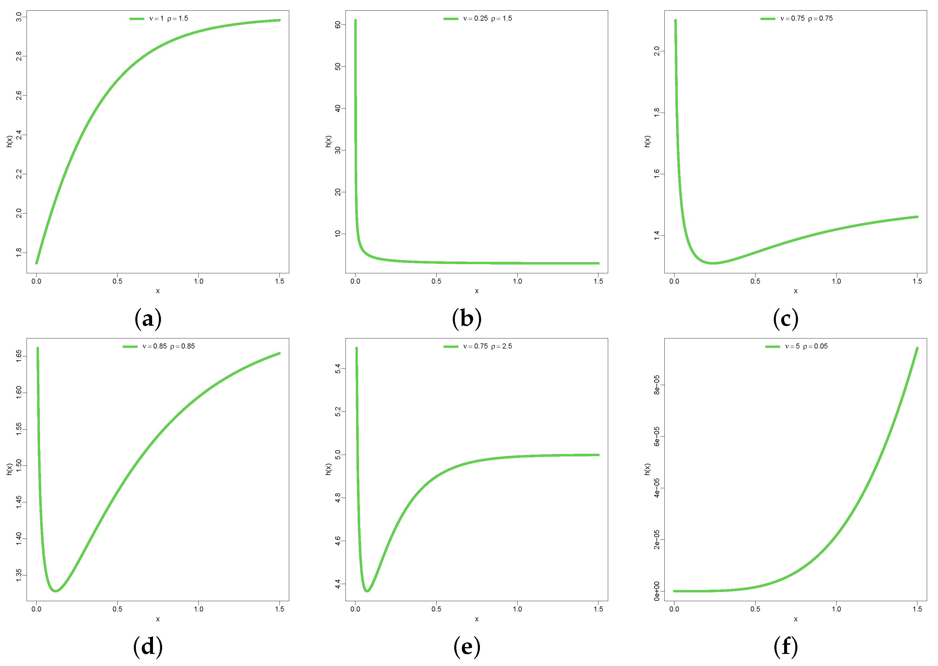
3. Baseline Extension: DUS Topp–Leone Exponential (DUS-TLE) Distribution
3.1. Extreme Behavior of the DUS-TLE Distribution
3.2. Mixture Representation
4. Characteristics
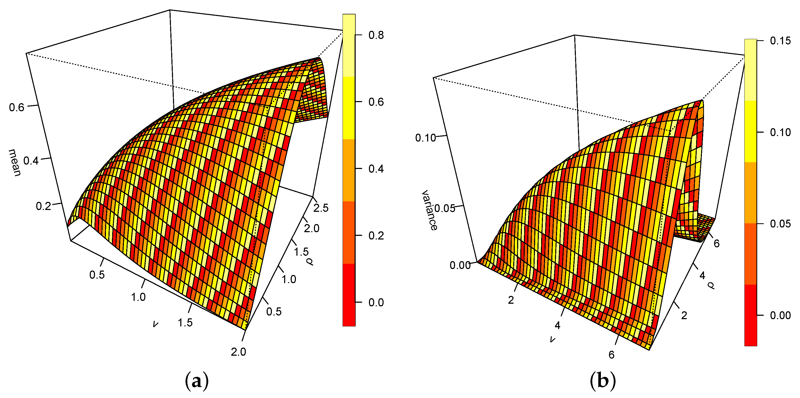
4.1. Moment
4.2. Quantile Function
4.3. Moment-Generating Function
4.4. Entropy
4.5. Order Statistic
5. Point Estimation
5.1. Maximum Likelihood Estimation
5.2. Least Squares Estimation (LSE)
5.3. Weighted Least Squares Estimation (WLSE)
5.4. Maximum Product of Spacing Estimation (MPS)
5.5. Cramér–von Mises Estimation (CVME)
5.6. Anderson–Darling Estimation (ADE)
5.7. Right-Tailed Anderson–Darling Estimation (RTADE)
5.8. Bayesian Estimation
6. Simulation
7. Applications
8. Final Remarks
Author Contributions
Funding
Data Availability Statement
Conflicts of Interest
References
- Marshall, A.W.; Olkin, I. A new method for adding a parameter to a family of distributions with application to the exponential and Weibull families. Biometrika 1997, 84, 641–652. [Google Scholar] [CrossRef]
- Eugene, N.; Lee, C.; Famoye, F. Beta-normal distribution and its applications. Commun. Stat.-Theory Methods 2002, 31, 497–512. [Google Scholar] [CrossRef]
- Cordeiro, G.M.; De Castro, M. A new family of generalized distributions. J. Stat. Comput. Simul. 2011, 81, 883–898. [Google Scholar] [CrossRef]
- Alzaatreh, A.; Lee, C.; Famoye, F. A new method for generating families of continuous distributions. Metron 2013, 71, 63–79. [Google Scholar] [CrossRef]
- Alzaghal, A.; Famoye, F.; Lee, C. Exponentiated TX family of distributions with some applications. Int. J. Stat. Probab. 2013, 2, 31. [Google Scholar] [CrossRef]
- Aljarrah, M.A.; Lee, C.; Famoye, F. On generating TX family of distributions using quantile functions. J. Stat. Distrib. Appl. 2014, 1, 1–17. [Google Scholar] [CrossRef]
- Tahir, M.; Cordeiro, G.M.; Alzaatreh, A.; Mansoor, M.; Zubair, M. The logistic-X family of distributions and its applications. Commun. Stat.-Theory Methods 2016, 45, 7326–7349. [Google Scholar] [CrossRef]
- Al-Mofleh, H. On generating a new family of distributions using the tangent function. Pak. J. Stat. Oper. Res. 2018, 14, 471–499. [Google Scholar] [CrossRef]
- Mahdavi, A.; Kundu, D. A new method for generating distributions with an application to exponential distribution. Commun. Stat.-Theory Methods 2017, 46, 6543–6557. [Google Scholar] [CrossRef]
- Gomes-Silva, F.S.; Percontini, A.; de Brito, E.; Ramos, M.W.; Venâncio, R.; Cordeiro, G.M. The odd Lindley-G family of distributions. Austrian J. Stat. 2017, 46, 65–87. [Google Scholar] [CrossRef]
- Ijaz, M.; Asim, S.M.; Alamgir; Farooq, M.; Khan, S.A.; Manzoor, S. A Gull Alpha Power Weibull distribution with applications to real and simulated data. PLoS ONE 2020, 15, e0233080. [Google Scholar] [CrossRef]
- Aldeni, M.; Lee, C.; Famoye, F. Families of distributions arising from the quantile of generalized lambda distribution. J. Stat. Distrib. Appl. 2017, 4, 1–18. [Google Scholar] [CrossRef]
- Yousof, H.M.; Altun, E.; Ramires, T.G.; Alizadeh, M.; Rasekhi, M. A new family of distributions with properties, regression models and applications. J. Stat. Manag. Syst. 2018, 21, 163–188. [Google Scholar] [CrossRef]
- Oramulu, D.O.; Alsadat, N.; Kumar, A.; Bahloul, M.M.; Obulezi, O.J. Sine generalized family of distributions: Properties, estimation, simulations and applications. Alex. Eng. J. 2024, 109, 532–552. [Google Scholar] [CrossRef]
- Zhao, W.; Khosa, S.K.; Ahmad, Z.; Aslam, M.; Afify, A.Z. Type-I heavy tailed family with applications in medicine, engineering and insurance. PLoS ONE 2020, 15, e0237462. [Google Scholar] [CrossRef] [PubMed]
- Kumar, D.; Singh, U.; Singh, S.K. A method of proposing new distribution and its application to Bladder cancer patients data. J. Stat. Appl. Pro. Lett 2015, 2, 235–245. [Google Scholar]
- Al-Noor, N.; Khaleel, M.; Mohammed, G. Theory and applications of Marshall Olkin Marshall Olkin Weibull distribution. J. Phys. Conf. Ser. 2021, 1999, 012101. [Google Scholar] [CrossRef]
- Feroze, N.; Tahir, U.; Noor-ul Amin, M.; Nisar, K.S.; Alqahtani, M.S.; Abbas, M.; Ali, R.; Jirawattanapanit, A. Applicability of modified weibull extension distribution in modeling censored medical datasets: A bayesian perspective. Sci. Rep. 2022, 12, 17157. [Google Scholar]
- Alyami, S.A.; Elbatal, I.; Alotaibi, N.; Almetwally, E.M.; Okasha, H.M.; Elgarhy, M. Topp–Leone modified Weibull model: Theory and applications to medical and engineering data. Appl. Sci. 2022, 12, 10431. [Google Scholar] [CrossRef]
- AbaOud, M.; Almuqrin, M.A. The weighted inverse Weibull distribution: Heavy-tailed characteristics, Monte Carlo simulation with medical application. Alex. Eng. J. 2024, 102, 99–107. [Google Scholar] [CrossRef]
- Bashir, S.; Masood, B.; Al-Essa, L.A.; Sanaullah, A.; Saleem, I. Properties, quantile regression, and application of bounded exponentiated Weibull distribution to COVID-19 data of mortality and survival rates. Sci. Rep. 2024, 14, 1–17. [Google Scholar] [CrossRef] [PubMed]
- Mazucheli, J.; Leiva, V.; Alves, B.; Menezes, A.F. A new quantile regression for modeling bounded data under a unit Birnbaum–Saunders distribution with applications in medicine and politics. Symmetry 2021, 13, 682. [Google Scholar] [CrossRef]
- Qura, M.E.; Fayomi, A.; Kilai, M.; Almetwally, E.M. Bivariate power Lomax distribution with medical applications. PLoS ONE 2023, 18, e0282581. [Google Scholar] [CrossRef]
- Tolba, A.H.; Onyekwere, C.K.; El-Saeed, A.R.; Alsadat, N.; Alohali, H.; Obulezi, O.J. A New Distribution for Modeling Data with Increasing Hazard Rate: A Case of COVID-19 Pandemic and Vinyl Chloride Data. Sustainability 2023, 15, 12782. [Google Scholar] [CrossRef]
- El-Morshedy, M.; Ahmad, Z.; Tag-Eldin, E.; Almaspoor, Z.; Eliwa, M.S.; Iqbal, Z. A new statistical approach for modeling the bladder cancer and leukemia patients data sets: Case studies in the medical sector. Math. Biosci. Eng. MBE 2022, 19, 10474–10492. [Google Scholar] [CrossRef] [PubMed]
- Rezaei, S.; Sadr, B.B.; Alizadeh, M.; Nadarajah, S. Topp–Leone generated family of distributions: Properties and applications. Commun. Stat.-Theory Methods 2017, 46, 2893–2909. [Google Scholar] [CrossRef]
- Rényi, A. On measures of entropy and information. Berkeley Symp. Math. Stat. Probab. 1961, 4, 547–562. [Google Scholar]
- Swain, J.J.; Venkatraman, S.; Wilson, J.R. Least-squares estimation of distribution functions in Johnson’s translation system. J. Stat. Comput. Simul. 1988, 29, 271–297. [Google Scholar] [CrossRef]
- Cheng, R.; Amin, N. Maximum Product of Spacings Estimation with Application to the Lognormal Distribution (Mathematical Report 79-1); University of Wales IST: Cardiff, UK, 1979. [Google Scholar]
- Varian, H.R. A Bayesian approach to real estate assessment. In Studies in Bayesian Econometrics and Statistics; In Honor of Leonard J. Savage; North-Holland Pub. Co.: Amsterdam, The Netherlands, 1975. [Google Scholar]
- Doostparast, M.; Akbari, M.G.; Balakrishna, N. Bayesian analysis for the two-parameter Pareto distribution based on record values and times. J. Stat. Comput. Simul. 2011, 81, 1393–1403. [Google Scholar] [CrossRef]
- Calabria, R.; Pulcini, G. Point estimation under asymmetric loss functions for left-truncated exponential samples. Commun. Stat.-Theory Methods 1996, 25, 585–600. [Google Scholar] [CrossRef]
- Brooks, S. Markov chain Monte Carlo method and its application. J. R. Stat. Soc. Ser. D Stat. 1998, 47, 69–100. [Google Scholar] [CrossRef]
- Van Ravenzwaaij, D.; Cassey, P.; Brown, S.D. A simple introduction to Markov Chain Monte–Carlo sampling. Psychon. Bull. Rev. 2018, 25, 143–154. [Google Scholar] [CrossRef] [PubMed]
- Mathers, B.M.; Degenhardt, L.; Bucello, C.; Lemon, J.; Wiessing, L.; Hickman, M. Mortality among people who inject drugs: A systematic review and meta-analysis. Bull. World Health Organ. 2013, 91, 102–123. [Google Scholar] [CrossRef] [PubMed]


| Author | Family of Distributions |
|---|---|
| Marshall and Olkin [1] | Marshall-Olkin-G family of distributions |
| Eugene et al. [2] | Beta-generated family of distributions |
| Cordeiro and De Castro [3] | Kumaraswamy-G family of distributions |
| Alzaatreh et al. [4] | T-X generator of families of continuous distributions |
| Alzaghal et al. [5] | Exponentiated TX family of distributions |
| Aljarrah et al. [6] | T-X family of distributions using quantile function |
| Tahir et al. [7] | The logistic-X family of distributions |
| Al-Mofleh [8] | Family of distributions using Tangent function |
| Mahdavi and Kundu [9] | Alpha-Power transformed family of distributions |
| Gomes-Silva et al. [10] | The odd Lindley-G family of distributions |
| Ijaz et al. [11] | Gull Alpha Power family of distributions |
| Aldeni et al. [12] | Family of distributions from quantile of generalized lambda distribution |
| Yousof et al. [13] | Burr-Hatke-G family of distributions |
| Oramulu et al. [14] | Sine generalized family of distributions |
| Zhao et al. [15] | Type-I heavy-tailed family of distributions |
| Kumar et al. [16] | Dinesh-Umesh-Sanjay (DUS) transformer |
| Method | Parameter | n = 25 | n = 75 | n = 150 | n = 200 | ||||
|---|---|---|---|---|---|---|---|---|---|
| Bias | RMSE | Bias | RMSE | Bias | RMSE | Bias | RMSE | ||
| ML | 0.30680 | 0.79234 | 0.09219 | 0.15996 | 0.04751 | 0.06450 | 0.02241 | 0.04550 | |
| 0.19930 | 0.42719 | 0.07518 | 0.12277 | 0.02882 | 0.05810 | 0.01743 | 0.04210 | ||
| MPS | 0.16516 | 0.38299 | 0.10045 | 0.12417 | 0.06373 | 0.05700 | 0.06527 | 0.04398 | |
| 0.22615 | 0.35714 | 0.10774 | 0.11675 | 0.07657 | 0.05963 | 0.06663 | 0.04421 | ||
| LS | 0.09827 | 0.82764 | 0.02863 | 0.21277 | 0.00911 | 0.08767 | 0.00373 | 0.06727 | |
| 0.01115 | 0.50545 | 0.00177 | 0.16889 | 0.01296 | 0.07683 | 0.00500 | 0.05955 | ||
| WLS | 0.11277 | 0.69385 | 0.04692 | 0.17505 | 0.02334 | 0.07285 | 0.01329 | 0.05418 | |
| 0.02160 | 0.44462 | 0.02784 | 0.13869 | 0.00389 | 0.06418 | 0.00673 | 0.04857 | ||
| CVM | 0.39490 | 1.47194 | 0.11051 | 0.25323 | 0.04837 | 0.09549 | 0.03287 | 0.07151 | |
| 0.22219 | 0.64390 | 0.07630 | 0.18369 | 0.02377 | 0.07914 | 0.02256 | 0.06118 | ||
| AD | 0.14738 | 0.60415 | 0.04846 | 0.16490 | 0.02249 | 0.07014 | 0.00990 | 0.05126 | |
| 0.06837 | 0.39784 | 0.03053 | 0.13086 | 0.00367 | 0.06305 | 0.00421 | 0.04702 | ||
| RTAD | 0.31941 | 1.41797 | 0.09683 | 0.25231 | 0.04417 | 0.11288 | 0.02378 | 0.07481 | |
| 0.12260 | 0.53070 | 0.05212 | 0.15721 | 0.01211 | 0.07803 | 0.00970 | 0.05390 | ||
| 0.55487 | 0.79907 | 0.78302 | 0.82006 | 0.98106 | 1.07951 | 1.04221 | 1.18535 | ||
| 0.36408 | 0.43646 | 0.60924 | 0.47901 | 0.75776 | 0.62920 | 0.80136 | 0.68520 | ||
| 0.62844 | 0.96311 | 0.82644 | 0.90727 | 1.01226 | 1.14775 | 1.06848 | 1.24556 | ||
| 0.41527 | 0.49233 | 0.63469 | 0.51296 | 0.77337 | 0.65376 | 0.81383 | 0.70580 | ||
| 0.48968 | 0.67696 | 0.74205 | 0.74333 | 0.95103 | 1.01621 | 1.01681 | 1.12884 | ||
| 0.31524 | 0.39025 | 0.58422 | 0.44712 | 0.74229 | 0.60538 | 0.78898 | 0.66508 | ||
| 0.52801 | 0.75787 | 0.76711 | 0.79237 | 0.97011 | 1.05709 | 1.03317 | 1.16570 | ||
| 0.34827 | 0.42386 | 0.60175 | 0.46978 | 0.75333 | 0.62247 | 0.79787 | 0.67957 | ||
| 0.47592 | 0.68470 | 0.73566 | 0.73951 | 0.94830 | 1.01332 | 1.01515 | 1.12717 | ||
| 0.31677 | 0.40067 | 0.58674 | 0.45168 | 0.74446 | 0.60911 | 0.79087 | 0.66838 | ||
| Method | Parameter | n = 25 | n = 75 | n = 150 | n = 200 | ||||
|---|---|---|---|---|---|---|---|---|---|
| Parameter | RMSE | Bias | RMSE | Bias | RMSE | Bias | RMSE | ||
| ML | 0.62385 | 3.27384 | 0.16483 | 0.42151 | 0.06410 | 0.18717 | 0.06424 | 0.13593 | |
| 0.09321 | 0.12497 | 0.03426 | 0.03025 | 0.01196 | 0.01452 | 0.01066 | 0.01049 | ||
| MPS | 0.23316 | 1.38440 | 0.17644 | 0.31953 | 0.12937 | 0.17002 | 0.09199 | 0.12226 | |
| 0.11930 | 0.10781 | 0.05938 | 0.02991 | 0.04167 | 0.01533 | 0.03233 | 0.01093 | ||
| LS | 0.33707 | 8.48090 | 0.05604 | 0.59520 | 0.00076 | 0.26796 | 0.01942 | 0.20502 | |
| 0.02555 | 0.15199 | 0.00156 | 0.04068 | 0.01050 | 0.02019 | 0.00488 | 0.01466 | ||
| WLS | 0.36863 | 6.75922 | 0.08602 | 0.48424 | 0.02274 | 0.21730 | 0.03906 | 0.16493 | |
| 0.00221 | 0.13786 | 0.01092 | 0.03388 | 0.00130 | 0.01648 | 0.00225 | 0.01205 | ||
| CVM | 0.95746 | 18.60741 | 0.20319 | 0.72522 | 0.06857 | 0.29164 | 0.07156 | 0.22052 | |
| 0.09027 | 0.18543 | 0.03629 | 0.04404 | 0.00809 | 0.02063 | 0.00908 | 0.01497 | ||
| AD | 0.31447 | 2.74304 | 0.08520 | 0.44165 | 0.02010 | 0.20800 | 0.03527 | 0.15791 | |
| 0.01695 | 0.11474 | 0.01178 | 0.03182 | 0.00164 | 0.01601 | 0.00148 | 0.01178 | ||
| RTAD | 0.88029 | 15.54110 | 0.15916 | 0.73757 | 0.07371 | 0.33997 | 0.06766 | 0.24252 | |
| 0.06513 | 0.16854 | 0.01888 | 0.04061 | 0.00597 | 0.02041 | 0.00552 | 0.01435 | ||
| 0.67844 | 1.41534 | 1.16084 | 1.84049 | 1.58896 | 2.84247 | 1.73921 | 3.30766 | ||
| 0.17403 | 0.09821 | 0.27674 | 0.10113 | 0.35621 | 0.13980 | 0.38250 | 0.15651 | ||
| 0.86690 | 1.98688 | 1.27584 | 2.19269 | 1.67748 | 3.16204 | 1.81700 | 3.61021 | ||
| 0.18657 | 0.10422 | 0.28257 | 0.10459 | 0.35980 | 0.14243 | 0.38541 | 0.15879 | ||
| 0.52400 | 1.07366 | 1.05666 | 1.55771 | 1.50633 | 2.56306 | 1.66593 | 3.03775 | ||
| 0.16176 | 0.09275 | 0.27095 | 0.09778 | 0.35264 | 0.13722 | 0.37960 | 0.15426 | ||
| 0.63330 | 1.32874 | 1.13397 | 1.77122 | 1.56968 | 2.77848 | 1.72276 | 3.24798 | ||
| 0.16671 | 0.09550 | 0.27347 | 0.09932 | 0.35428 | 0.13843 | 0.38096 | 0.15533 | ||
| 0.54643 | 1.18074 | 1.08097 | 1.64005 | 1.53140 | 2.65406 | 1.69001 | 3.13116 | ||
| 0.15213 | 0.09051 | 0.26693 | 0.09576 | 0.35042 | 0.13571 | 0.37787 | 0.15298 | ||
| Method | Parameter | n = 25 | n = 75 | n = 150 | n = 200 | ||||
|---|---|---|---|---|---|---|---|---|---|
| Bias | RMSE | Bias | RMSE | Bias | RMSE | Bias | RMSE | ||
| ML | 0.56269 | 2.21375 | 0.14932 | 0.33317 | 0.06334 | 0.15198 | 0.06078 | 0.10010 | |
| 0.08839 | 0.08023 | 0.02728 | 0.02183 | 0.01380 | 0.01088 | 0.01137 | 0.00755 | ||
| MPS | 0.20649 | 0.92956 | 0.15207 | 0.25429 | 0.10942 | 0.13591 | 0.07790 | 0.08988 | |
| 0.09463 | 0.06639 | 0.05121 | 0.02174 | 0.03174 | 0.01107 | 0.02492 | 0.00770 | ||
| LS | 0.26941 | 2.59778 | 0.05353 | 0.49264 | 0.00398 | 0.21157 | 0.02736 | 0.15190 | |
| 0.00146 | 0.09369 | 0.00403 | 0.03038 | 0.00537 | 0.01459 | 0.00004 | 0.01061 | ||
| WLS | 0.28144 | 2.09340 | 0.07386 | 0.38236 | 0.02694 | 0.17503 | 0.03967 | 0.11799 | |
| 0.01467 | 0.08091 | 0.00525 | 0.02481 | 0.00276 | 0.01216 | 0.00501 | 0.00858 | ||
| CVM | 0.77818 | 5.01773 | 0.18445 | 0.60104 | 0.06550 | 0.23040 | 0.07385 | 0.16454 | |
| 0.10205 | 0.12013 | 0.02794 | 0.03274 | 0.01037 | 0.01502 | 0.01179 | 0.01095 | ||
| AD | 0.32248 | 1.79021 | 0.07763 | 0.34288 | 0.02692 | 0.17012 | 0.03674 | 0.11330 | |
| 0.03265 | 0.07505 | 0.00757 | 0.02311 | 0.00300 | 0.01198 | 0.00433 | 0.00837 | ||
| RTAD | 0.61784 | 4.30160 | 0.16501 | 0.61153 | 0.07456 | 0.26461 | 0.06682 | 0.17531 | |
| 0.05472 | 0.09869 | 0.01813 | 0.02927 | 0.00966 | 0.01436 | 0.00836 | 0.01012 | ||
| 0.73799 | 1.42996 | 1.13777 | 1.72789 | 1.48489 | 2.47283 | 1.60244 | 2.80185 | ||
| 0.18034 | 0.08540 | 0.25661 | 0.08445 | 0.31653 | 0.10983 | 0.33589 | 0.12038 | ||
| 0.89581 | 1.91333 | 1.23470 | 2.01506 | 1.55800 | 2.71767 | 1.66601 | 3.02873 | ||
| 0.18951 | 0.08978 | 0.26092 | 0.08681 | 0.31918 | 0.11155 | 0.33803 | 0.12185 | ||
| 0.60603 | 1.11966 | 1.04915 | 1.49168 | 1.41613 | 2.25559 | 1.54223 | 2.59701 | ||
| 0.17134 | 0.08132 | 0.25233 | 0.08215 | 0.31389 | 0.10813 | 0.33376 | 0.11893 | ||
| 0.69768 | 1.34820 | 1.11335 | 1.66632 | 1.46748 | 2.41898 | 1.58770 | 2.75259 | ||
| 0.17407 | 0.08301 | 0.25376 | 0.08299 | 0.31485 | 0.10876 | 0.33455 | 0.11947 | ||
| 0.61987 | 1.20545 | 1.06514 | 1.54928 | 1.43289 | 2.31414 | 1.55837 | 2.65612 | ||
| 0.16157 | 0.07853 | 0.24807 | 0.08011 | 0.31146 | 0.10664 | 0.33185 | 0.11767 | ||
| Method | Parameter | n = 25 | n = 75 | n = 150 | n = 200 | ||||
|---|---|---|---|---|---|---|---|---|---|
| Bias | RMSE | Bias | RMSE | Bias | RMSE | Bias | RMSE | ||
| ML | 0.28923 | 0.68747 | 0.06090 | 0.09121 | 0.02797 | 0.04395 | 0.02971 | 0.03158 | |
| 0.15552 | 0.26020 | 0.04898 | 0.06401 | 0.02221 | 0.03398 | 0.01980 | 0.02398 | ||
| MPS | 0.10818 | 0.32147 | 0.09584 | 0.07624 | 0.06335 | 0.04088 | 0.04342 | 0.02897 | |
| 0.15872 | 0.21058 | 0.08758 | 0.06293 | 0.05709 | 0.03460 | 0.04318 | 0.02425 | ||
| LS | 0.15703 | 1.21881 | 0.01157 | 0.13360 | 0.00077 | 0.06268 | 0.01339 | 0.04779 | |
| 0.00977 | 0.30922 | 0.00269 | 0.08758 | 0.00524 | 0.04632 | 0.00210 | 0.03293 | ||
| WLS | 0.16585 | 0.98256 | 0.02444 | 0.10774 | 0.01211 | 0.05068 | 0.02204 | 0.03891 | |
| 0.02039 | 0.27083 | 0.01369 | 0.07252 | 0.00736 | 0.03832 | 0.01135 | 0.02743 | ||
| CVM | 0.41648 | 2.14639 | 0.07808 | 0.15745 | 0.03274 | 0.06761 | 0.03750 | 0.05116 | |
| 0.16217 | 0.38709 | 0.05317 | 0.09518 | 0.02228 | 0.04798 | 0.02276 | 0.03406 | ||
| AD | 0.17118 | 0.63199 | 0.02501 | 0.09611 | 0.01150 | 0.04934 | 0.02031 | 0.03756 | |
| 0.05173 | 0.23968 | 0.01678 | 0.06785 | 0.00712 | 0.03757 | 0.01017 | 0.02686 | ||
| RTAD | 0.39883 | 2.79388 | 0.06030 | 0.17341 | 0.02779 | 0.07340 | 0.03029 | 0.05555 | |
| 0.11914 | 0.33689 | 0.02793 | 0.08349 | 0.01324 | 0.04499 | 0.01298 | 0.03174 | ||
| 0.58809 | 0.76387 | 0.72901 | 0.69061 | 0.85761 | 0.81980 | 0.89613 | 0.87370 | ||
| 0.38965 | 0.35068 | 0.52297 | 0.33972 | 0.60835 | 0.40263 | 0.63299 | 0.42603 | ||
| 0.64248 | 0.88184 | 0.76112 | 0.74964 | 0.87973 | 0.86175 | 0.91461 | 0.90996 | ||
| 0.41984 | 0.38310 | 0.53801 | 0.35681 | 0.61749 | 0.41416 | 0.64026 | 0.43551 | ||
| 0.53868 | 0.66966 | 0.69842 | 0.63746 | 0.83617 | 0.78035 | 0.87815 | 0.83929 | ||
| 0.36052 | 0.32193 | 0.50812 | 0.32337 | 0.59927 | 0.39138 | 0.62575 | 0.41672 | ||
| 0.56585 | 0.72909 | 0.71558 | 0.66894 | 0.84857 | 0.80368 | 0.88869 | 0.85982 | ||
| 0.37747 | 0.34041 | 0.51706 | 0.33346 | 0.60486 | 0.39837 | 0.63023 | 0.42253 | ||
| 0.52248 | 0.66583 | 0.68897 | 0.62740 | 0.83059 | 0.77217 | 0.87386 | 0.83257 | ||
| 0.35319 | 0.32107 | 0.50523 | 0.32117 | 0.59787 | 0.38992 | 0.62472 | 0.41557 | ||
| 4.6 | 0.9 | 1.8 | 1.4 | 0.2 | 3.9 | 1.8 | 0.8 | 2.0 | 0.8 | 1.6 | 0.8 | 2.0 |
| 1.6 | 0.5 | 0.1 | 2.5 | 2.4 | 0.6 | 1.1 | 0.7 | 1.7 | 1.0 | 1.7 | 2.5 | 3.5 |
| 0.3 | 0.9 | 2.3 | 0.5 | 1.5 | 5.1 | 0.2 | 1.5 | 3.3 | 1.4 | 3.3 |
| S | Min | Max | IQR | Sk | Ku | Range | |||
|---|---|---|---|---|---|---|---|---|---|
| 1.677297 | 1.512492 | 1.229834 | 0.1 | 5.1 | 1.5 | 1.017765 | 3.539668 | 0.2 | 5 |
| Dist | NLL | AIC | CAIC | BIC | HQIC | W | A | KS | p-Value | (Shape) | (Scale) |
|---|---|---|---|---|---|---|---|---|---|---|---|
| DUS-TLE | 53.58 | 111.159 | 111.512 | 114.381 | 112.295 | 0.029 | 0.180 | 0.089 | 0.9331 | 1.5482 | 0.4679 |
| TIHTE | 54.0 | 111.992 | 112.345 | 115.214 | 113.128 | 0.032 | 0.194 | 0.108 | 0.7860 | 0.2857 | 2.6509 |
| Gamma | 53.66 | 111.337 | 111.690 | 114.559 | 112.473 | 0.033 | 0.204 | 0.092 | 0.9144 | 1.7613 | 0.9769 |
| GIE | 62.73 | 129.466 | 129.819 | 132.688 | 130.602 | 0.294 | 1.785 | 0.211 | 0.0731 | 1.2723 | 0.8900 |
| Lnorm | 56.19 | 116.701 | 117.054 | 119.923 | 117.837 | 0.104 | 0.659 | 0.112 | 0.7413 | 0.2970 | 0.9011 |
| EIE | 54.68 | 113.356 | 113.709 | 116.578 | 114.492 | 0.062 | 0.387 | 0.146 | 0.4101 | 0.2409 | 0.3679 |
| Lomax | 56.57 | 117.149 | 117.502 | 120.371 | 118.285 | 0.033 | 0.205 | 0.160 | 0.3026 | 20051134 | 11813144 |
| 2.01 | 6.32 | 3.52 | 2.15 | 5.42 | 2.04 | 2.77 | 2.26 | 1.95 | 1.00 | 2.45 | 0.74 | 0.98 |
| 1.27 | 2.77 | 3.68 | 1.18 | 1.09 | 1.60 | 0.57 | 3.33 | 0.91 | 7.14 | 2.08 | 3.85 | 1.99 |
| 7.76 | 2.52 | 1.47 | 4.67 | 4.22 | 1.92 | 1.59 | 4.08 | 2.02 | 0.84 | 6.85 | 2.18 | 2.04 |
| 1.05 | 2.91 | 1.37 | 2.43 | 2.28 | 3.74 | 1.30 | 1.59 | 1.83 | 3.85 | 6.30 | 4.83 | 0.50 |
| 3.40 | 2.33 | 4.25 | 3.49 | 2.12 | 0.83 | 0.54 | 3.23 | 4.50 | 0.71 | 0.48 | 2.30 | 7.73 |
| S | Min | Max | IQR | Sk | Ku | Range | |||
|---|---|---|---|---|---|---|---|---|---|
| 2.724923 | 3.351263 | 1.830645 | 0.48 | 7.76 | 2.31 | 1.124585 | 3.689323 | 0.23 | 7.28 |
| Distribution | LL | AIC | CAIC | BIC | HQIC | W | A | KS | p-Value | (Shape) | (Scale) |
|---|---|---|---|---|---|---|---|---|---|---|---|
| DUS-TLE | 119.55 | 243.104 | 243.297 | 247.453 | 244.820 | 0.054 | 0.351 | 0.081 | 0.7835 | 2.2928 | 0.3518 |
| TIHTE | 121.68 | 246.150 | 246.344 | 250.499 | 247.866 | 0.142 | 0.473 | 0.113 | 0.3788 | 0.1172 | 3.7800 |
| Weibull | 120.43 | 244.861 | 245.055 | 249.210 | 246.577 | 0.081 | 0.532 | 0.095 | 0.5983 | 3.0561 | 1.5949 |
| Lnorm | 119.74 | 243.961 | 243.454 | 247.610 | 244.960 | 0.056 | 0.354 | 0.116 | 0.3416 | 0.7311 | 0.6950 |
| Gumbel | 121.8 | 247.599 | 247.793 | 251.948 | 249.315 | 0.078 | 0.531 | 0.088 | 0.6987 | 1.9259 | 1.2892 |
Disclaimer/Publisher’s Note: The statements, opinions and data contained in all publications are solely those of the individual author(s) and contributor(s) and not of MDPI and/or the editor(s). MDPI and/or the editor(s) disclaim responsibility for any injury to people or property resulting from any ideas, methods, instructions or products referred to in the content. |
© 2024 by the authors. Licensee MDPI, Basel, Switzerland. This article is an open access article distributed under the terms and conditions of the Creative Commons Attribution (CC BY) license (https://creativecommons.org/licenses/by/4.0/).
Share and Cite
Ekemezie, D.-F.N.; Anyiam, K.E.; Kayid, M.; Balogun, O.S.; Obulezi, O.J. DUS Topp–Leone-G Family of Distributions: Baseline Extension, Properties, Estimation, Simulation and Useful Applications. Entropy 2024, 26, 973. https://doi.org/10.3390/e26110973
Ekemezie D-FN, Anyiam KE, Kayid M, Balogun OS, Obulezi OJ. DUS Topp–Leone-G Family of Distributions: Baseline Extension, Properties, Estimation, Simulation and Useful Applications. Entropy. 2024; 26(11):973. https://doi.org/10.3390/e26110973
Chicago/Turabian StyleEkemezie, Divine-Favour N., Kizito E. Anyiam, Mohammed Kayid, Oluwafemi Samson Balogun, and Okechukwu J. Obulezi. 2024. "DUS Topp–Leone-G Family of Distributions: Baseline Extension, Properties, Estimation, Simulation and Useful Applications" Entropy 26, no. 11: 973. https://doi.org/10.3390/e26110973
APA StyleEkemezie, D.-F. N., Anyiam, K. E., Kayid, M., Balogun, O. S., & Obulezi, O. J. (2024). DUS Topp–Leone-G Family of Distributions: Baseline Extension, Properties, Estimation, Simulation and Useful Applications. Entropy, 26(11), 973. https://doi.org/10.3390/e26110973