The Circumstance-Driven Bivariate Integer-Valued Autoregressive Model

Abstract

The novel circumstance-driven bivariate integer-valued autoregressive (CuBINAR) model for non-stationary count time series is proposed. The non-stationarity of the bivariate count process is defined by a joint categorical sequence, which expresses the current state of the process. Additional cross-dependence can be generated via cross-dependent innovations. The model can also be equipped with a marginal bivariate Poisson distribution to make it suitable for low-count time series. Important stochastic properties of the new model are derived. The Yule–Walker and conditional maximum likelihood method are adopted to estimate the unknown parameters. The consistency of these estimators is established, and their finite-sample performance is investigated by a simulation study. The scope and application of the model are illustrated by a real-world data example on sales counts, where a soap product in different stores with a common circumstance factor is investigated.

1. Introduction

Integer-valued time series data are encountered in many fields in practice, such as epidemiology, insurance, finance, and quality control (see [1] for a comprehensive survey). There are many approaches to model such count data. One pioneering approach is to use a random thinning operator as a substitute of the multiplication in the traditional autoregressive (AR) model to construct an integer-valued autoregressive (INAR) model (see [2,3]). The first-order INAR (INAR(1)) model is defined as follows:

$$\begin{array}{c}\hfill X_t=\alpha \circ X_{t-1}+{\epsilon }_t,\end{array}$$

(1)

$t\in {\mathbb{N}}_{+}$, where $\alpha \circ X_{t-1}$ is defined as $\alpha \circ X_{t-1}={\displaystyle \sum _{i=1}^{X_{t-1}}}{Y}_i$, with $\left\{Y_i\right\}$ being a sequence of independent and identically distributed (i. i. d.) Bernoulli random variables with parameter $\alpha \in [0,1)$. The innovations ${\epsilon }_t$ are i. i. d. count random variables, i.e., having the range ${\mathbb{N}}_0=\{0,1,\dots \}$, where the default choice is a Poisson distribution for ${\epsilon }_t$ [3]. Many researchers have generalized the basic INAR(1) model to better fit real data. To handle overdispersion or zero-inflation features in data, the negative-binomial, geometric or zero-inflated Poisson distribution have been proposed to replace the Poisson distribution of innovation term ${\epsilon }_t$ (see [1] for details and references). Also, different types of thinning operator have been proposed in the literature (see [4] for a survey). Other proposals generalize the model from the view of the model structure. Thyregod et al. [5] first proposed the self-exciting threshold (SET) integer-valued model, which is also studied in [6]. A comprehensive introduction to SET-INAR models can be found in [7].

The aforementioned articles focus on stationary count time series. To handle the non-stationary case, ref. [8] applied the difference method to non-stationary count data and introduced the signed binomial thinning operator to allow for negative values after differencing. Nastić et al. [9] constructed the random-environment INAR(1) model to characterize non-stationarity in integer-valued time series, where the parameters in the model are influenced by different states of the environment, the evolution of which is defined through a selection mechanism from a Markov chain. Laketa et al. [10] generalized this work to a p-th order model.

Nowadays, there is increasing interest in multivariate integer-valued time series models, where most contributions focus on the bivariate case. Such types of data are commonly encountered in real-world applications. For example, ref. [11] consider the number of daytime and nighttime accidents in a certain area, which are at distinct levels but present cross-correlation due to the same road conditions. Latour [12] first proposed a general multivariate INAR(1) model and proved the existence and relevant properties of the model. Further model properties have been studied by [13]. The bivariate INAR(1) model introduced by [11] is defined as

$$\begin{array}{c}\hfill {\mathit{X}}_t=\mathit{A}\circ {\mathit{X}}_{t-1}+{\mathit{R}}_t=\left[\begin{array}{cc}{\alpha }_1& 0\\ 0& {\alpha }_2\end{array}\right]\circ \left[\begin{array}{c}{X}_{1,t-1}\\ X_{2,t-1}\end{array}\right]+\left[\begin{array}{c}{\epsilon }_{1,t}\\ {\epsilon }_{2,t}\end{array}\right],\end{array}$$

(2)

where “∘” is the binomial thinning operator defined as in (1), with ${\alpha }_1,{\alpha }_2\in [0,1)$. ${\epsilon }_{i,t}$ is the innovation term of the i-th series, $i=1,2$. The role of the $\mathit{A}\circ$ is the usual matrix multiplication, and it also keeps the properties of the binomial thinning operation. Regarding further research on bivariate INAR(1) models, we refer to the work of [14,15], while we refer to the work of [16,17,18] for research on bivariate integer-valued moving average (INMA(1)) models. In addition, ref. [19] introduced a bivariate model for integer-valued time series with a finite range of counts. Yu et al. [20] introduced the new bivariate random-coefficient integer-valued autoregressive (BRCINAR(1)) model to allow the coefficients to be random. Although the present article concentrates on thinning-based models for count time series (which allow us to specify the marginal distribution of $\left({\mathit{X}}_t\right)$), it should also be briefly mentioned that different approaches have been proposed in the literature. Regression-type models for (bivariate) count time series (where the conditional distributions of ${\mathit{X}}_t|{\mathit{X}}_{t-1},\dots$ are specified rather than the marginal ones) have been proposed by, e.g., [21,22,23]. In contrast, ref. [24] derive a multivariate count time series model with Poisson marginal distributions from underlying multivariate Gaussian time series.

Non-stationarity is an important feature of real-world time series data, whether for one-dimensional or multi-dimensional data. The change in external factors may change the structure or level in the data. There has not been much work to explore the non-stationarity of bivariate count time series. One main problem is the distribution of the model, which becomes complicated with increasing dimension. We propose a new model to characterize the non-stationarity in bivariate integer-valued time series. Inspired by [9,25], we suppose the parameters in the model to be affected by the different states of the circumstance, to characterize the intrinsic nature of non-stationarity in the data. In contrast to [25], the novel model is able to incorporate additional cross-dependence, and it is also suitable for low-count time series having a bivariate Poisson marginal distribution (see Remark 3 for further details). In Section 2, we propose the new first-order circumstance-driven bivariate INAR (CuBINAR(1)) model, and establish its stochastic properties. Estimation methods and their asymptotic properties are discussed in Section 3. In Section 4, the performance of the estimators is evaluated by a simulation study. A real-data application is presented in Section 5. Summary and conclusions are given in Section 6.

2. Model Construction

In this section, we introduce the new non-stationary CuBINAR(1) model, where the bivariate count random variable ${\mathit{X}}_t$ at time t is not only influenced by ${\mathit{X}}_{t-1}$, but also by the underlying circumstance state $s_t$ as we define in (3).

Definition 1.

The CuBINAR(1) process $\left({\mathit{X}}_t\right)$ with range ${\mathbb{N}}_0^2$ is defined by the recursive scheme

$$\begin{array}{c}\hfill {\mathit{X}}_t\left(s_t\right)=\mathit{A}\circ {\mathit{X}}_{t-1}\left(s_{t-1}\right)+{\mathit{\epsilon }}_t(s_t,s_{t-1}).\end{array}$$

(3)

The model can be rewritten in matrix form as

$$\left[\begin{array}{c}{X}_{1,t}\left(s_t\right)\\ X_{2,t}\left(s_t\right)\end{array}\right]=\left[\begin{array}{cc}{\alpha }_1& 0\\ 0& {\alpha }_2\end{array}\right]\circ \left[\begin{array}{c}{X}_{1,t-1}\left(s_{t-1}\right)\\ X_{2,t-1}\left(s_{t-1}\right)\end{array}\right]+\left[\begin{array}{c}{\epsilon }_{1,t}(s_t,s_{t-1})\\ {\epsilon }_{2,t}(s_t,s_{t-1})\end{array}\right],$$

i.e., the i-th component of the vector ${\mathit{X}}_t\left(s_t\right)$ satisfies

$$\begin{array}{c}\hfill X_{i,t}\left(s_t\right)={\alpha }_i\circ X_{i,t}\left(s_{t-1}\right)+{\epsilon }_{i,t}(s_t,s_{t-1}),i=1,2,t=2,\dots ,n.\end{array}$$

Here, $s_t$ represents the state at time t with possible values in $\mathit{S}=\{1,2,\dots ,S\}$, where $S⩾2$ is total number of states. $X_{i,t}\left(s_t\right)$ is the t-th observation of the i-th series depending on the state $s_t$, and ${\epsilon }_{i,t}(s_t,s_{t-1})$ is the corresponding innovation term depending on the states $s_t$ and $s_{t-1}$. In addition, ${\mathit{\epsilon }}_t(s_t,s_{t-1})$ is independent of $\mathit{A}\circ {\mathit{X}}_{t-1}\left(s_{t-1}\right)$ and ${\mathit{X}}_k\left(s_k\right)$ for $k<t$, where the definition of the binomial thinning operator “∘” is given after (1).

Remark 1.

We assume the different states of the circumstance are already realized. In the simulation part, we first need to generate the sample path of the states. To characterize the variation of the states, we adopt a Markov chain to generate it: given the initial probability vector $p_0=(p_1,\dots ,p_S)$ and transition matrix $P=\left(\begin{array}{ccc}{p}_{11}& \cdots & p_{1S}\\ ⋮& \ddots & ⋮\\ p_{S1}& \cdots & p_{SS}\end{array}\right)$, the sample path of the states can be obtained. In real-data analysis, we first need to know the states of the observations. In the data example discussed in Section 5, the sequence of states is defined according to a possible sales promotion.

In the subsequent Proposition 1, we introduce the important special case of a CuBINAR(1) process having a bivariate Poisson marginal distribution (thus abbreviated as Poi-CuBINAR(1)). More precisely, $\left({\mathit{X}}_t\right)$ is said to follow the Poi-CuBINAR(1) model if $\{X_{1,t},X_{2,t}\}\sim \mathrm{BPoi}({\lambda }_1\left(s_t\right),{\lambda }_2\left(s_t\right),\varphi )$ for appropriately chosen parameter values (see Remark 2 below). Here, we use the same definition of the BPoi-distribution as in [11,13], i.e., the parameters of $\mathit{X}\sim \mathrm{BPoi}({\lambda }_1,{\lambda }_2,\varphi )$ are defined as the mean of $X_1$, mean of $X_2$, and covariance between $X_1,X_2$, respectively. So the probability generating function (PGF) of $\mathit{X}$ would be given by

$$E[a_1^{X_1}·a_2^{X_2}]=exp\{{\lambda }_1(a_1-1)+{\lambda }_2(a_2-1)+\varphi (a_1-1)(a_2-1)\}.$$

It shall be shown that, in analogy to the univariate Poi-INAR(1) model [4], BPoi-observations are achieved by assuming BPoi-innovations.

Proposition 1.

Let $\left({\mathit{X}}_t\right)$ be a CuBINAR(1) process according to Definition 1. Then, $\left({\mathit{X}}_t\right)$ constitutes a Poi-CuBINAR(1) process with $\{X_{1,t},X_{2,t}\}\sim \mathrm{BPoi}({\lambda }_1\left(s_t\right),{\lambda }_2\left(s_t\right),\varphi )$ if the distribution of the model’s innovation term satisfies

$$\{{\epsilon }_{1,t}(s_t,s_{t-1}),{\epsilon }_{2,t}(s_t,s_{t-1})\}\sim \mathrm{BPoi}({\lambda }_1\left(s_t\right)-{\lambda }_1\left(s_{t-1}\right){\alpha }_1,{\lambda }_2\left(s_t\right)-{\lambda }_2\left(s_{t-1}\right){\alpha }_2,{\varphi }^{*}),$$

where ${\varphi }^{*}=\varphi (1-{\alpha }_1{\alpha }_2)$.

For the detailed proof, we refer to Appendix B. Note that for the derivation of Proposition 1, it is crucial that $\mathit{A}$ is a diagonal matrix. While Definition 1 could generally be extended to a non-diagonal $\mathit{A}$, we would lose the marginal BPoi-property (see also [13] for analogous results in the stationary case). In fact, the components would then not follow univariate INAR(1) models any more.

Remark 2.

We must ensure the parameters of the $\mathrm{BPoi}({\lambda }_1\left(s_t\right),{\lambda }_2\left(s_t\right),\varphi )$-distribution in Proposition 1 are truly positive, i.e., ${\lambda }_i\left(s\right)-{\lambda }_i\left(r\right){\alpha }_i-\varphi +\varphi {\alpha }_1{\alpha }_2>0$ holds for $i=1,2$ and $r,s\in S$ at same time, where s and r are the realizations of $s_t$ and $s_{t-1}$, respectively. Hence, there are $2·S^2$ inequalities that need to be satisfied simultaneously.

Remark 3.

As already indicated in Section 1, the novel CuBINAR(1) model is constructed in a similar way as the bivariate “random environment INAR(1) model” proposed by [25], referred to as RE-BINAR(1) hereafter. But, there are also noteworthy differences between these two models. First, for the BRrNGINAR(1) model of [25], cross-correlation between the two series is solely caused by the common state while their innovation sequences are mutually independent. Our CuBINAR(1) model, by contrast, allows for additional cross-correlation being caused by the cross-correlated innovation term. For example, in case of the Poi-CuBINAR(1) model, the innovation term $\{{\epsilon }_{1,t}(s_t,s_{t-1}),{\epsilon }_{2,t}(s_t,s_{t-1})\}$ stems from a bivariate Poisson distribution, also leading to a bivariate Poisson distribution for $\{X_{1,t}\left(s_t\right),X_{2,t}\left(s_t\right)\}$ (see Proposition 1). Then, choosing $\varphi >0$ leads to additional cross-correlation, while mutually independent innovations series are included as the special case $\varphi =0$. Altogether, the user has more flexibility to fit the model to given time series data.

Second, ref. [25] construct their model based on the negative-binomial thinning operator and geometric marginal distributions, so the model is particularly useful for overdispersed counts. Our CuBINAR(1) model, by contrast, uses binomial thinnings. As discussed by [4], binomial thinnings can also be used to generate common overdispersed marginal distributions (including the geometric one). But, in addition, the equidispersed Poisson distribution is also possible, as it is often observed for low-counts time series. In the special case of the Poi-CuBINAR(1) model introduced in Proposition 1, the process is equipped with a marginal bivariate Poisson distribution. Altogether, we believe that our novel CuBINAR(1) model constitutes a valuable complement to existing models for non-stationary bivariate count time series.

The following proposition provides some (conditional) moment properties of the Poi-CuBINAR(1) model, which shall useful to obtain the Yule–Walker estimators.

Proposition 2.

Let $\left({\mathit{X}}_t\right)$ be the Poi-CuBINAR(1) process according to Proposition 1. Let us denote the means of $X_{i,t}\left(s_t\right)$, $X_{i,t-1}\left(s_{t-1}\right)$, and ${\epsilon }_{i,t}(s_t,s_{t-1})$ as ${\lambda }_i\left(s_t\right)$, ${\lambda }_i\left(s_{t-1}\right)$, and ${\mu }_i(s_t,s_{t-1})$, respectively, for $i=1,2$. Then, the following assertions hold:

(i) 

$E[X_{i,t}\left(s_t\right)\mid X_{i,t-1}\left(s_{t-1}\right)]={\alpha }_i·X_{i,t-1}\left(s_{t-1}\right)+{\mu }_i(s_t,s_{t-1})$;

$E\left[X_{i,t}\left(s_t\right)\right]={\lambda }_i\left(s_t\right)$;

(ii) 

$Var\left(X_{i,t}\left(s_t\right)\right)={\lambda }_i\left(s_t\right)$;

$cov(X_{i,t}\left(s_t\right),X_{i,t-1}\left(s_{t-1}\right))={\alpha }_i·{\lambda }_i\left(s_{t-1}\right)$;

(iii) 

$cov(X_{1,t}\left(s_t\right),X_{2,t}\left(s_t\right))=\varphi$;

$cov(X_{1,t}\left(s_t\right),X_{2,t-k}\left(s_{t-k}\right))={\alpha }_1^k·\varphi$.

For the proof of Proposition 2, see Appendix C.

3. Parameter Estimation

In this section, we consider the Yule–Walker (YW) method and the conditional maximum likelihood (CML) method to estimate the parameter values of the Poi-CuBINAR(1) model.

3.1. Yule–Walker Estimation

From now on, let us use the following notations, for $i=1,2$ and $r,s\in \mathit{S}$:

$$\begin{array}{cc}\hfill {\mu }_i\left(s\right)& =E[X_{i,t}\left(s_t\right)\mid s_t=s],\hfill \\ \hfill {\gamma }_{ii,0}\left(s\right)& =Var(X_{it}\left(s_t\right)\mid s_t=s),\hfill \\ \hfill {\gamma }_{12,0}\left(s\right)& =cov(X_{1,t}\left(s_t\right),X_{2,t}\left(s_t\right)\mid s_t=s),\hfill \\ \hfill {\gamma }_i(r,s)& =cov(X_{i,t}\left(s_t\right),X_{i,t-1}\left(s_{t-1}\right)\mid s_{t-1}=r,s_t=s).\hfill \end{array}$$

(4)

For the Poi-CuBINAR(1) model, the $X_{i,t}$ are Poisson-distributed, so ${\mu }_i\left(s\right)$ is equal to ${\gamma }_{ii,0}\left(s\right)$.

Given the realized states, the corresponding sample moments are as follows:

$$\begin{array}{cc}\hfill {\widehat{\mu }}_i\left(s\right)& \hfill =\frac{1}{n_s}\sum _{t=1}^n{X}_{i,t}\left(s_t\right){\mathbb{1}}_{\{s_t=s\}},\hfill \end{array}$$

(5)

$$\begin{array}{cc}\hfill {\widehat{\gamma }}_{ij,0}\left(s\right)& \hfill =\frac{1}{n_s}\sum _{t=1}^n(X_{i,t}\left(s_t\right)-{\widehat{\mu }}_i\left(s\right))(X_{j,t}\left(s_t\right)-{\widehat{\mu }}_j\left(s\right)){\mathbb{1}}_{\{s_t=s\}},\hfill \end{array}$$

(6)

$$\begin{array}{cc}\hfill {\widehat{\gamma }}_i(r,s)& \hfill =\frac{1}{n_{r,s}}\sum _{t=2}^n(X_{i,t}\left(s_t\right)-{\widehat{\mu }}_i\left(s\right))(X_{i,t-1}\left(s_{t-1}\right)-{\widehat{\mu }}_i\left(r\right)){\mathbb{1}}_{\{s_{t-1}=r,s_t=s\}}.\hfill \end{array}$$

(7)

In Equation (6), $i=j$ leads to ${\widehat{\gamma }}_{ii,0}\left(s\right)$, which is the empirical conditional variance given the state s, and which estimates ${\gamma }_{ii,0}\left(s\right)$. Otherwise, it equals the empirical conditional cross-covariance and thus estimates ${\gamma }_{12,0}\left(s\right)$. $n_s={\sum }_{t=1}^n{\mathbb{1}}_{\{s_t=s\}}$ is the sample size under state s, $n_{r,s}={\sum }_{t=2}^n{\mathbb{1}}_{\{s_{t-1}=r,s_t=s\}}$ the one under the condition that the state at t equals s and that at $t-1$ equals r. ${\mathbb{1}}_A$ denotes the indicator function, which is equal to 1 (0) if A is true (false).

Remark 4.

The parameters ϕ and ${\alpha }_i$ can be expressed by the following equations:

$$\begin{array}{cc}\hfill \varphi & \hfill =\sum _{s=1}^S\frac{n_s}{n}·{\gamma }_{12,0}\left(s\right),\hfill \end{array}$$

(8)

$$\begin{array}{cc}\hfill {\alpha }_i& \hfill =\sum _{r=1}^S\sum _{s=1}^S\frac{n_{r,s}}{n}·\frac{{\gamma }_i(r,s)}{{\gamma }_{ii,0}\left(r\right)},\hfill \end{array}$$

(9)

see Appendix D for the proof. Equations (8) and (9) can be used to define estimators of ϕ and ${\alpha }_i$, respectively.

Following Remark 4, we define the Yule–Walker estimators as follows:

$$\begin{array}{cc}\hfill {\widehat{\alpha }}_i^{yw}& \hfill =\sum _{r=1}^S\sum _{s=1}^S\frac{n_{r,s}}{n-1}\frac{{\widehat{\gamma }}_i(r,s)}{{\widehat{\gamma }}_{ii,0}\left(r\right)},\hfill \end{array}$$

(10)

$$\begin{array}{cc}\hfill {\widehat{\lambda }}_i{\left(s\right)}^{yw}& \hfill ={\widehat{\mu }}_i\left(s\right),s\in S,\hfill \end{array}$$

(11)

$$\begin{array}{cc}\hfill {\widehat{\varphi }}^{yw}& \hfill =\sum _{s=1}^S\frac{n_s}{n}{\widehat{\gamma }}_{12,0}\left(s\right).\hfill \end{array}$$

(12)

In next theorem, we prove that these Yule–Walker estimators are consistent.

Theorem 1.

The Yule–Walker estimators ${\widehat{\alpha }}_i^{yw}$, ${\widehat{\lambda }}_i{\left(s\right)}^{yw}$ and ${\widehat{\varphi }}^{yw}$, $i=1,2$, $s\in S$ defined in Equations (10)–(12) are consistent.

The proof of Theorem 1 is provided by Appendix E.

3.2. Conditional Maximum Likelihood Estimation

From the first-order Markov property of the CuBINAR(1) model according to Definition 1, the conditional log-likelihood function is expressed as

$$\begin{array}{c}\hfill \mathcal{L}=\sum _{t=2}^{n}logP({\mathit{X}}_t\left(s_t\right)\mid {\mathit{X}}_{t-1}\left(s_{t-1}\right)),\end{array}$$

where $P({\mathit{X}}_t\left(s_t\right)\mid {\mathit{X}}_{t-1}\left(s_{t-1}\right))$ is the transition probability given the realized states. It has the following expression, where, for simplicity, we omit the states $s_t,s_{t-1}$ in parentheses after ${\mathit{X}}_t,{\mathit{X}}_{t-1}$:

$$\begin{array}{cc}\hfill P({\mathit{X}}_t\mid {\mathit{X}}_{t-1})& \hfill =P(X_{1,t}=x_{1,t},X_{2,t}=x_{2,t}\mid X_{1,t-1}=x_{1,t-1},X_{2,t-1}=x_{2,t-1})\hfill \\ \hfill & \hfill =\sum _{k=0}^{min(x_{1,t},x_{1,t-1})}\sum _{l=0}^{min(x_{2,t},x_{2,t-1})}\left(\genfrac{}{}{0pt}{}{x_{1,t-1}}{k}\right)·{\alpha }_1^k·{(1-{\alpha }_1)}^{x_{1,t-1}-k}\hfill \\ \hfill & \hfill ·\left(\genfrac{}{}{0pt}{}{x_{2,t-1}}{l}\right)·{\alpha }_2^l·{(1-{\alpha }_2)}^{x_{2,t-1}-l}·f(x_{1,t}-k,x_{2,t}-l),\hfill \end{array}$$

(13)

where $f(x_{1,t}-k,x_{2,t}-l)=e^{-({\lambda }_1^{*}+{\lambda }_2^{*}+{\varphi }^{*})}{\displaystyle \sum _{i=0}^{min(x_{1,t}-k,x_{2,t}-l)}}\frac{{{\lambda }_1^{*}}^{(x_{1,t}-k-i)}{{\lambda }_2^{*}}^{(x_{2,t}-l-i)}{{\varphi }^{*}}^i}{(x_{1,t}-k-i)!(x_{2,t}-l-i)!i!}$. Here, ${\lambda }_1^{*}={\lambda }_1\left(s_t\right)-{\lambda }_1\left(s_{t-1}\right){\alpha }_1-{\varphi }^{*}$, ${\lambda }_2^{*}={\lambda }_2\left(s_t\right)-{\lambda }_2\left(s_{t-1}\right){\alpha }_2-{\varphi }^{*}$, and ${\varphi }^{*}=\varphi -\varphi {\alpha }_1{\alpha }_2$. The CML estimates are computed by applying a numerical optimization routine to the log-likelihood function $\mathcal{L}$. Based on the inverse of the numerical Hessian, one can then calculate approximate standard errors (see Remark B.2.1.2 in [1] for details.)

4. Simulation Study

In this section, we conduct a simulation study to evaluate the performance of the YW and CML estimators. The standard errors and biases of the estimators are calculated based on 10,000 replications, where the sample sizes are $n\in \{300,900,1500,2100\}$. Since we assume that the states of the circumstance are already realized, we first need to generate the circumstance states for each replication run, which is performed via the Markov chain approach described in Remark 1. In order to implement this, the initial probability vector and the transition probability matrix need to be specified.

Two different scenarios are considered. In the first scenario, we assume that the observations are driven by three different states of the circumstance, in which case we also consider two different types of transition probability matrix: one with initial probability vector $p_0^{\left(1\right)}=(0.33,0.33,0.34)$ and transition probability matrix $\left(\begin{array}{ccc}0.4& 0.3& 0.3\\ 0.3& 0.4& 0.3\\ 0.3& 0.3& 0.4\end{array}\right)$, the other with $p_0^{\left(2\right)}=(0.6,0.3,0.1)$ and $\left(\begin{array}{ccc}0.6& 0.3& 0.1\\ 0.1& 0.6& 0.3\\ 0.3& 0.1& 0.6\end{array}\right)$. Furthermore, three different parameter groups are considered:

(a)

$({\alpha }_1,{\alpha }_2,\varphi ,{\varphi }^{*},{\lambda }_1\left(1\right),{\lambda }_1\left(2\right),{\lambda }_1\left(3\right),{\lambda }_2\left(1\right),{\lambda }_2\left(2\right),{\lambda }_3\left(3\right))$

$=(0.15,0.2,0.5,0.485,1,2,3,4,5,6)$;

(b)

$({\alpha }_1,{\alpha }_2,\varphi ,{\varphi }^{*},{\lambda }_1\left(1\right),{\lambda }_1\left(2\right),{\lambda }_1\left(3\right),{\lambda }_2\left(1\right),{\lambda }_2\left(2\right),{\lambda }_3\left(3\right))$

$=(0.15,0.5,0.5,0.4625,1,2,3,4,5,6)$;

(c)

$({\alpha }_1,{\alpha }_2,\varphi ,{\varphi }^{*},{\lambda }_1\left(1\right),{\lambda }_1\left(2\right),{\lambda }_1\left(3\right),{\lambda }_2\left(1\right),{\lambda }_2\left(2\right),{\lambda }_3\left(3\right))$

$=(0.4,0.25,1,0.9,3,4,5,2,3,4)$.

In the second scenario, we suppose the circumstance to only have two states. Two different transition probability matrices are set, namely $\left(\begin{array}{cc}0.4& 0.6\\ 0.6& 0.4\end{array}\right)$ and $\left(\begin{array}{cc}0.8& 0.2\\ 0.2& 0.8\end{array}\right)$, respectively, and the corresponding initial probability vectors are $(0.5,0.5)$ and $(0.3,0.7)$.

(d)

$({\alpha }_1,{\alpha }_2,\varphi ,{\varphi }^{*},{\lambda }_1\left(s_1\right),{\lambda }_1\left(s_2\right),{\lambda }_2\left(s_1\right),{\lambda }_2\left(s_2\right))$

$=(0.15,0.2,0.5,0.4625,1,3,3,5)$;

(e)

$({\alpha }_1,{\alpha }_2,\varphi ,{\varphi }^{*},{\lambda }_1\left(s_1\right),{\lambda }_1\left(s_2\right),{\lambda }_2\left(s_1\right),{\lambda }_2\left(s_2\right))$

$=(0.25,0.5,1,0.875,2,4,5,7)$.

Note that the ${\alpha }_1,{\alpha }_2$ in all parameters groups satisfy the constraints in Remark 2.

The estimation results of the YW and CML estimators are presented in Table A1, Table A2, Table A3, Table A4, Table A5, Table A6, Table A7, Table A8, Table A9 and Table A10 in Appendix A. It can be seen that if the sample size increases, all estimates converge to the true parameter values: the standard errors and biases decrease towards to 0, confirming the consistency of the estimators. Comparing the finite-sample properties among the YW and CML approaches, it becomes clear that the additional computational effort required for CML also leads to an improved performance. The CML estimates are less biased and less dispersed, where the additional gain in performance is particularly large for the dependence parameters ${\alpha }_1$, ${\alpha }_2$, and $\varphi$. So if possible, the CML approach should be preferred for parameter estimation.

5. A Real-Data Example

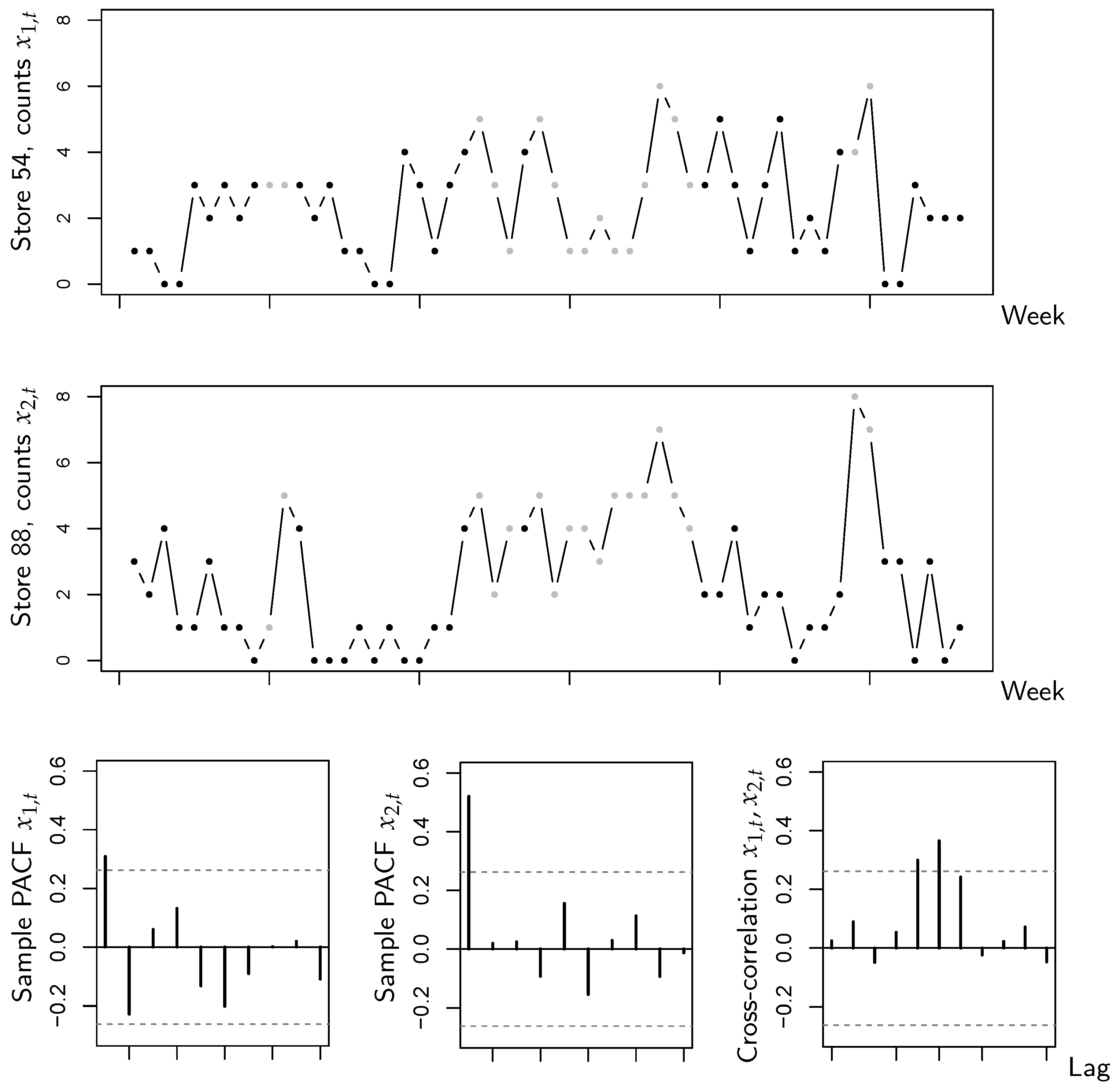
In this section, we analyze data referring to the number of sold items of a soap product (category “wsoa” in Dominick’s Data (https://www.chicagobooth.edu/research/kilts/datasets/dominicks, accessed on 10 November 2021) from the James M. Kilts Center, University of Chicago, Booth School of Business), which are counted on a weekly basis. We focus on the product “Level 200 Bath 6 BA” (code number 1111132012) in the soap category, and we consider the bivariate count time series for stores 54 and 88 in the period April 14, 1994, to 4 May 1995 (weeks 240–295, $n=56$). The movement files also provide information on a sales promotion for the product. There are three types of promotion (labeled ‘B’, ‘C’ and ‘S’), which we summarized into one category, namely “sales promotion—yes or no” (yes: state 1; no: state 2). As the number of sold items might be affected by whether the product is under promotion or not, the action of promotion can be seen as a potential circumstance-driving factor. It is also worth mentioning that ref. [26] analyzed count data from the soap category (product “Zest White Water”), but using a Hidden-Markov model instead (i.e., they did not utilize the information about sales promotion).

The data are shown in Figure 1, with the counts in state 1 being plotted in gray color. The PACFs indicate an AR(1)-like autocorrelation structure, and we are also concerned with a substantial extent of cross-correlation. However, it can be seen that for both sub-series, the counts under sales promotion are at a higher level than without sales promotion. This indicates that the sales promotion is helpful to stimulate the number of sold items, and might thus be a relevant circumstance state. If computing the state-dependent sample means and variances (as required for YW estimation anyway, recall Section 3.1), one gets the values of Table 1. Comparing the means across the states, the visual impression from Figure 1 is confirmed, which is that counts are larger (in the mean) in state 1 (promotion) than in state 2. But, it is also interesting to compare the corresponding means and variances. Keeping in mind that the sub-series are rather short, such that variations are natural, the overall impression is that means and variances are reasonably close to each other, i.e., a model with state-dependent equidispersion could be suitable for the data. Together with the aforementioned substantial extent of cross-correlation, it is thus reasonable to try the novel CuBINAR(1) model for the sales counts data.

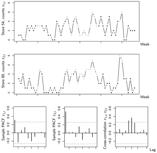
Figure 1. Bivariate sales counts from Section 5: time series plots, sample PACFs, and cross-correlations of both sub-series. The dots in the time series plots are printed in gray (black) color if the state equals 1 (2).

Table 1. State-dependent sample means and variances of sales counts data.

	State 1		State 2
	Mean	Var	Mean	Var
$x_{1,t}$	3.111	3.046	2.132	2.063
$x_{2,t}$	4.500	3.206	1.553	1.876

To evaluate the performance of our new model, we fit the CuBINAR(1) model to the data, and as competitors, we consider the classical (stationary) Poi-BINAR(1) model (2) of [11] on the one hand, and the RE-BINAR(1) model of [25] (recall Remark 3) on the other hand. Model fitting is performed via the CML approach, where the numerical optimization is initialized by the YW estimates (recall Section 3 and Section 4). The estimation results are summarized in Table 2. We also computed approximate standard errors as described in Section 3.2, but since the time series is rather short, the dependence parameters ${\widehat{\alpha }}_1,{\widehat{\alpha }}_2,\widehat{\varphi }$ are not significant on a 5%-level. As the estimates ${\widehat{\lambda }}_i\left(s_t\right)$ in the CuBINAR(1) model refer to the marginal mean of $X_{i,t}\left(s_t\right)$, we convert the means of the BINAR(1)’s innovation terms ${\epsilon }_{i,t}$ into the marginal mean of $X_{i,t}$ in order to make the results comparable. That is, the estimates ${\widehat{\lambda }}_1$ and ${\widehat{\lambda }}_2$ of the BINAR(1) model represent the marginal means of $X_{i,t}$. We can see that the CuBINAR(1)’s estimates ${\widehat{\lambda }}_i\left(1\right)$, $i=1,2$, of both sub-series under state 1 are larger than those under state 2, which confirms that the sales promotion increases the number of sold items. The corresponding ${\widehat{\lambda }}_i$ of the BINAR(1) model are located between ${\widehat{\lambda }}_i\left(1\right)$ and ${\widehat{\lambda }}_i\left(2\right)$, whereas the RE-BINAR(1)’s estimates differ quite a lot in some cases (and also deviate from the sample means in Table 1). It is also interesting to note that the values of ${\widehat{\alpha }}_1,{\widehat{\alpha }}_2,\widehat{\varphi }$ are smaller for CuBINAR(1) than for BINAR(1), which is reasonable as part of the CuBINAR(1)’s dependence is explained by the circumstance states. Furthermore, the estimate $\widehat{\varphi }$ is clearly larger than zero, i.e., the ability of the CuBINAR(1) model to incorporate additional cross-dependence (recall Remark 3) turns out to be beneficial in view of the substantial extent of cross-correlation observed in Figure 1.

Table 2. CML parameter estimates of sales counts data.

Model	CuBINAR(1)		RE-BINAR(1)		BINAR(1)
	${\widehat{\alpha }}_1$	0.265	${\widehat{\alpha }}_1$	0.609	${\widehat{\alpha }}_1$	0.288
	${\widehat{\alpha }}_2$	0.215	${\widehat{\alpha }}_2$	0.619	${\widehat{\alpha }}_2$	0.396
	${\widehat{\lambda }}_1\left(1\right)$	2.929	${\widehat{\lambda }}_1\left(1\right)$	1.823	${\widehat{\lambda }}_1$	2.480
	${\widehat{\lambda }}_1\left(2\right)$	2.266	${\widehat{\lambda }}_1\left(2\right)$	2.090
	${\widehat{\lambda }}_2\left(1\right)$	4.187	${\widehat{\lambda }}_2\left(1\right)$	3.589	${\widehat{\lambda }}_2$	2.467
	${\widehat{\lambda }}_2\left(2\right)$	1.586	${\widehat{\lambda }}_2\left(2\right)$	1.322
	$\widehat{\varphi }$	0.250			$\widehat{\varphi }$	0.312

To assess the performance of the fitted models, we first compare the root mean square errors (RMSEs) between the observations and predicted values. More precisely, the RMSE values are the square-roots of sums of the form ${\sum }_t{\left(x_{i,t}-E\left[X_{i,t}\left(s_t\right)\right|x_{i,t-1}\left(s_{t-1}\right)]\right)}^2$, divided by the number of summands. Here, we distinguish two cases. The in-sample RMSE is computed by using the model fits of Table 2 and by summing for $t=2,\dots ,n$. For the out-of-sample RMSEs, we omitted the last 10 observations during model fitting, and then the sum was taken about $t=n-9,\dots ,n$. Obviously, the RMSE performances of the CuBINAR(1) model are better than those of both the RE-BINAR(1) and BINAR(1) model.

In addition to the RMSE, we also adopt scoring rules and Akaike’s information criterion (AIC) for model choice. Regarding the scoring rules, we use the logarithmic score defined as

$$\begin{array}{c}\hfill S_{ls}(p_{·\mid x_{t-1}},x_t):=-ln{p}_{x_t\mid x_{t-1}}.\end{array}$$

The mean score $\frac{1}{n-1}{\displaystyle \sum _{t=2}^n}{S}_{ls}(p_{·\mid x_{t-1}},x_t)$ is used to assess the overall performance of the model. Smaller score values indicate that the predictive distribution provided by the fitted model is in better agreement with the true predictive distribution, which implies a better fit of the model. Analogously, smaller values of the AIC indicate a better model. From Table 3, we recognize that both the AIC and the logarithmic score of the CuBINAR(1) model are smaller than those of the competing models. Altogether, the CuBINAR(1) model clearly outperforms both competitors. Regarding the BINAR(1) model, our newly proposed model can better fit the sales count data by utilizing the dependence to the underlying circumstance. The superior performance compared to the RE-BINAR(1) model can be explained from two types of sample properties noted in the beginning of this section. First, the data exhibit notable cross-correlation, but only the CuBINAR(1) model has an additional cross-dependence parameter. Second, conditioned on the different states, the sales counts are close to equidispersion, which is accounted for by the CuBINAR(1)’s Poisson distributions. The RE-BINAR(1) model with its geometric distributions, by contrast, is designed for strongly overdispersed data, but which does not apply to the sales counts data.

Table 3. AIC, logarithmic score, and RMSE of sales counts data.

Model:	AIC	Logarithmic Score	in-RMSE	out-RMSE
$\mathbf{CuBINAR}\left(\mathbf{1}\right)$	399.8	3.507	$x_{1,t}$: 1.468	1.849
			$x_{2,t}$: 1.456	1.864
$\mathbf{RE}-\mathbf{BINAR}\left(\mathbf{1}\right)$	427.8	3.780	$x_{1,t}$: 1.607	2.163
			$x_{2,t}$: 1.566	2.139
$\mathbf{BINAR}\left(\mathbf{1}\right)$	418.1	3.710	$x_{1,t}$: 1.504	1.887
			$x_{2,t}$: 1.761	2.408

While CuBINAR(1) model performs best among the candidate models, it remains to assess its overall model adequacy. First, we analyzed the corresponding standardized Pearson residuals defined by

$$\frac{x_{i,t}-E\left[X_{i,t}\left(s_t\right)\right|x_{i,t-1}\left(s_{t-1}\right)]}{\sqrt{Var\left(X_{i,t}\left(s_t\right)\right|x_{i,t-1}\left(s_{t-1}\right))}}\mathrm{for}i=1,2\mathrm{and}t=2,3,\dots$$

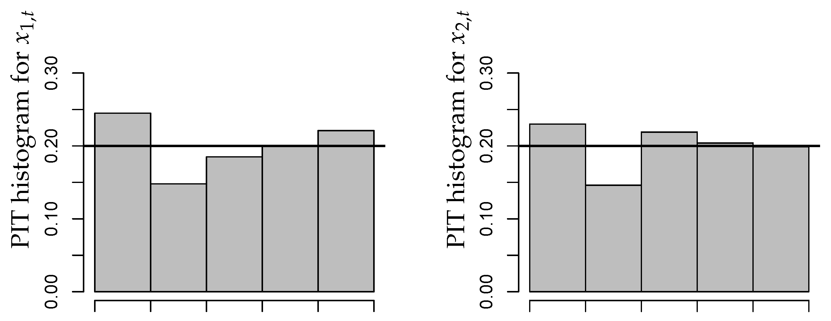
A summary of results is provided by Figure 2. As explained in Section 2.4 of [1], the residuals of an adequate model should have a mean close to zero, a variance close to one, and they should not be autocorrelated. From Figure 2, we conclude that these criteria are satisfied in good approximation. It is also worth noting that there exist no significant cross-correlations between the residuals series. We also computed the PIT histograms for the fitted CuBINAR(1) model, as these are another common approach for checking the model adequacy (see Section 2.4 in [1]). But, since the sample size is rather short, the PIT histograms in Figure 3 look a bit “spiky”. Nevertheless, they exhibit no systematic deviation from uniformity, such as a (inverse) U-shape. Therefore, they do not contradict to the fitted CuBINAR(1) model. Altogether, our novel CuBINAR(1) model appears to adequately describe the bivariate sales counts data.

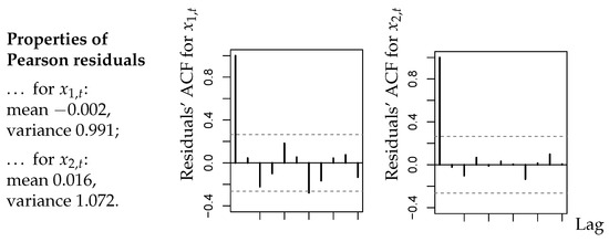
Figure 2. Bivariate sales counts from Section 5: sample means, variances, and ACFs of Pearson residuals with respect to fitted CuBINAR(1) model.

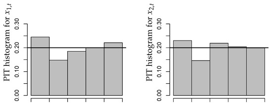
Figure 3. Bivariate sales counts from Section 5: PIT histograms with respect to fitted CuBINAR(1) model.

6. Conclusions

In this paper, we proposed the new circumstance-driven bivariate INAR(1) model, which can be applied to bivariate count time series that have different marginal means caused by an underlying circumstance factor. Important stochastic properties of the new model were discussed. We applied and analyzed the Yule–Walker and conditional maximum likelihood method to estimate the unknown parameter values. The consistency of the estimators was also confirmed by our simulation study where the estimation results converge quickly to the true parameter values with increasing sample size. For the presented real-data application on sales counts, our new model outperforms the ordinary BINAR(1) model. As a possible direction for future research, we suggest equipping models for multivariate count time series with a self-exciting threshold mechanism, similar to the recent work by [27]. Another important topic would be the case where the states cannot be observed (latent states, in analogy to the Hidden-Markov model [26]). Then, the CuBINAR(1)’s model definition and estimation approaches need to be adapted, which should be performed in future research.

References

- Weiß, C. An Introduction to Discrete-Valued Time Series; Wiley: Chichester, UK, 2018. [Google Scholar]
- McKenzie, E. Some simple models for discrete variate time series. JAWRA J. Am. Water Resour. Assoc. 1985, 21, 645–650. [Google Scholar] [CrossRef]
- Al-Osh, M.; Alzaid, E. First-order integer-valued autoregressive (INAR(1)) process. J. Time Ser. Anal. 1987, 8, 314–324. [Google Scholar] [CrossRef]
- Weiß, C. Thinning operations for modeling time series of counts—A survey. AStA Adv. Stat. Anal. 2008, 92, 319–334. [Google Scholar] [CrossRef]
- Thyregod, P.; Carstensen, N.; Madsen, H.; Arnbjerg-Nielsen, K. Integer-valued autoregressive models for tipping bucket rainfall measurements. Environmetrics 1999, 10, 395–411. [Google Scholar] [CrossRef]
- Monteiro, M.; Scotto, M.G.; Pereira, I. Integer-valued self-exciting threshold autoregressive processes. Commun. Stat.-Theory Methods 2012, 41, 2717–2737. [Google Scholar] [CrossRef]
- Möller, T.; Weiß, C. Threshold models for integer-valued time series with infinite or finite range. In Stochastic Models, Statistics and Their Applications; Steland, A., Rafajłowicz, E., Szajowski, K., Eds.; Springer: Wrocław, Poland, 2015; pp. 327–334. [Google Scholar]
- Kim, H.; Park, Y. A non-stationary integer-valued autoregressive model. Stat. Pap. 2008, 49, 485–502. [Google Scholar] [CrossRef]
- Nastić, A.; Laketa, P.; Ristić, M. Random environment integer-valued autoregressive process. J. Time Ser. Anal. 2016, 37, 267–287. [Google Scholar] [CrossRef]
- Laketa, P.; Nastić, A.; Ristić, M. Generalized random environment INAR models of higher order. Mediterr. J. Math. 2016, 15, 9. [Google Scholar] [CrossRef]
- Pedeli, X.; Karlis, D. A bivariate INAR(1) process with application. Stat. Model. 2011, 11, 325–349. [Google Scholar] [CrossRef]
- Latour, A. The multivariate GINAR(p) process. Adv. Appl. Probab. 1997, 29, 228–248. [Google Scholar] [CrossRef]
- Pedeli, X.; Karlis, D. Some properties of multivariate INAR(1) processes. Comput. Stat. Data Anal. 2013, 67, 213–225. [Google Scholar] [CrossRef]
- Karlis, D.; Pedeli, X. Flexible Bivariate INAR(1) Processes Using Copulas. Commun. Stat.-Theory Methods 2013, 42, 723–740. [Google Scholar] [CrossRef]
- Santos, C.; Pereira, I.; Scotto, M. On the theory of periodic multivariate INAR processes. Stat. Pap. 2019, 69, 1291–1348. [Google Scholar]
- Khan, N.; Sunecher, Y.; Jowaheer, V. Modelling a non-stationary BINAR(1) Poisson process. J. Stat. Comput. Simul. 2016, 86, 3106–3126. [Google Scholar] [CrossRef]
- Sunecher, Y.; Khan, N.; Jowaheer, V. BINMA(1) model with COM-Poisson innovations: Estimation and application. Commun. Stat.-Simul. Comput. 2018, 49, 1631–1652. [Google Scholar] [CrossRef]
- Silva, I.; Silva, M.E.; Torres, C. Inference for bivariate integer-valued moving average models based on binomial thinning operation. J. Appl. Stat. 2020, 47, 2546–2564. [Google Scholar] [CrossRef] [PubMed]
- Scotto, M.; Weiß, C.; Silva, M.; Pereira, I. Bivariate binomial autoregressive models. J. Multivariate Anal. 2014, 125, 233–251. [Google Scholar] [CrossRef]
- Yu, M.; Wang, D.; Yang, K.; Liu, Y. Bivariate first-order random coefficient integer-valued autoregressive processes. J. Stat. Plan. Inference 2020, 204, 153–176. [Google Scholar] [CrossRef]
- Cui, Y.; Zhu, F. A new bivariate integer-valued GARCH model allowing for negative cross-correlation. Test 2018, 27, 428–452. [Google Scholar] [CrossRef]
- Silva, R.B.; Barreto-Souza, W. Flexible and robust mixed Poisson INGARCH models. J. Time Ser. Anal. 2019, 40, 788–814. [Google Scholar] [CrossRef]
- Piancastelli, L.S.C.; Barreto-Souza, W.; Ombao, H. Flexible bivariate INGARCH process with a broad range of contemporaneous correlation. J. Time Ser. Anal. 2023, 44, 206–222. [Google Scholar] [CrossRef]
- Livsey, J.; Lund, R.; Kechagias, S.; Pipiras, V. Multivariate integer-valued time series with flexible autocovariances and their application to major hurricane counts. Ann. Appl. Stat. 2018, 12, 408–431. [Google Scholar] [CrossRef]
- Popović, P.; Laketa, P.; Nasti, A. Forecasting with two generalized integer-valued autoregressive processes of order one in the mutual random environment. SORT-Stat. Oper. Res. Trans. 2019, 43, 355–384. [Google Scholar]
- MacDonald, I.; Zucchini, W. Hidden Markov models for discrete-valued time series. In Handbook of Discrete-Valued Time Series; Davis, R.A., Holan, S.H., Lund, R., Ravishanker, N., Eds.; CRC Press: Boca Raton, FL, USA, 2016; pp. 267–286. [Google Scholar]
- Contreras-Reyes, J.E. Information quantity evaluation of multivariate SETAR processes of order one and applications. Stat. Pap. 2023, in press. [CrossRef]
- White, H. Asymptotic Theory For Econometricians; Academic Press: London, UK, 2001. [Google Scholar]
Disclaimer/Publisher’s Note: The statements, opinions and data contained in all publications are solely those of the individual author(s) and contributor(s) and not of MDPI and/or the editor(s). MDPI and/or the editor(s) disclaim responsibility for any injury to people or property resulting from any ideas, methods, instructions or products referred to in the content. |
© 2024 by the authors. Licensee MDPI, Basel, Switzerland. This article is an open access article distributed under the terms and conditions of the Creative Commons Attribution (CC BY) license (https://creativecommons.org/licenses/by/4.0/).