Design of a Robust Synchronization-Based Topology Observer for Complex Delayed Networks with Fixed and Adaptive Coupling Strength

Abstract

Network topology plays a key role in determining the characteristics and dynamical behaviors of a network. But in practice, network topology is sometimes hidden or uncertain ahead of time because of network complexity. In this paper, a robust-synchronization-based topology observer (STO) is proposed and applied to solve the problem of identifying the topology of complex delayed networks (TICDNs). In comparison to the existing literature, the proposed STO does not require any prior knowledge about the range of topological parameters and does not have strict limits on topology type. Furthermore, the proposed STO is suitable not only for networks with fixed coupling strength, but also for networks with adaptive coupling strength. Finally, a few comparison examples for TICDNs are used to verify the feasibility and efficiency of the proposed STO, and the results show that the proposed STO outperforms the other methods.

1. Introduction

As we all know, complex networks have become ubiquitous as models of various real-world systems. In order to analyze the statistical properties and behaviors of networks, researchers have extensively studied the topology and dynamics of complex networks [1,2]. Ref. [1] explored the statistical mechanics of network topology and dynamics, while ref [2] analyzed the impact of time-delay coupling on the synchrony of gene networks composed of coupled oscillators. Furthermore, numerous case studies have been conducted on different real-world networks, yielding insights from various perspectives. These studies have encompassed predicting collective behaviors [3,4], applications in control systems [5,6], and other areas. These achievements have made significant contributions to the theory of multi-connected models, which significantly increases the working efficiency of networked systems. But it is worth noting that much complex network research is based on the assumption that the network topology is known or predefined. However, with the high security and secrecy requirements of complex networks in practice, due to the strict industrial system protection mechanism, some parameters are difficult to measure. Therefore, we focus primarily on identifying the topology of complex networks in this paper.

Generally speaking, in the most complex networks, time lag is unavoidable due to the time lag characteristics of certain physical devices and real-world networks. In order to simulate more realistic networks, there has been pioneering research in the topology identification of complex delayed networks (TICDNs). Some initial results have been obtained. A number of the existing approaches, such as optimization-based strategies [7,8,9,10,11,12], compressed sensing technologies [13,14,15,16], and synchronization-based methods [17,18,19,20,21,22,23,24,25], are widely used to deal with unknown topology. The main idea of an optimization-based strategy is to convert the TICDN into an optimization problem and then solve the problem with various classical or evolutionary algorithms. In [8], a chaotic ant swarm intelligence algorithm (CASIA) was investigated to identify topology. Other classical algorithms, such as weighted least square (WLS) algorithms, for the identification of the topology of uncertain networks were studied in [10]. The unknown topological structure of power systems was studied in [11], which was formulated as a weighted least square problem and solved by a distributed sub-gradient algorithm (DSA). On the other hand, compressed sensing technology uses a special sampling mechanism to recover the original signal for the TICDN, which has the advantage of requiring less measurement data. In [13,14], the researchers devoted their efforts to study the topology recovery of single and multiple complex networks based on compressive sensing and Taylor expansion. In [15], the authors proposed a method combining compressive sensing and graph theory to identify smart grids.

However, while optimization-based strategies accurately estimate unknown topology, their computational costs are often high. Compressed sensing does not apply to some non-sparse networks, and the sparse representation of the signals must be incoherent, which is not straightforward to achieve in real networks. Along with the development of modern control theorems, the TICDN problem based on synchronization methods has gradually attracted the attention of researchers in recent years, This method has been explained in detail and proven rigorously via the Lyapunov stability theory [26], Linear Matrix Inequalities (LMI) [27], and many other techniques [28,29]. Unknown topology can be identified via the proposed STO, and the response–drive networks have to actualize synchronization. In the literature mentioned above, topology observers are designed for complex networks via the sliding mode control technique [18], the adaptive-feedback approach [19,20,21,22,23,24], and the line feedback approach [25]. With further research, considering the large scale of some networks, pinning control has played a certain role because only a small number of nodes require control. In [30], the authors addressed the synchronization problem of linear coupled complex networks via aperiodically intermittent pinning control. The authors of [31] mainly studied the synchronization of neural networks via the pinning control of certain vital nodes. The authors of [32] studied the pinning synchronization problem for a class of complex networks using a moment-based analysis approach. Recently, in order to save on the cost of identification and investigate the benefits of the pinning mechanism, the authors of [33,34] investigated the problem of identifying the partial topology for undirected networks.

Compared to the optimization strategy and compressed sensing-based technology, the synchronization-based method avoids the need for both huge computations and a priori knowledge about topological parameters. Meanwhile, unknown topology is not necessarily required to be symmetric, irreducible, or sparse. Owing to these features, more unknown network models have been further investigated via the synchronization-based method [35,36,37]. On the other hand, it should be noted that the majority of the above-mentioned studies focus on the coupling strength being a known constant coefficient in network models. This may sometimes be unsatisfactory, as some real-world networks are characterized by evolution [38]. That is to say, the coupling strength is adaptively tuned based on the environment and human activities in various cases. In real life, there are some examples of complex networks with adaptive coupling strength. For instance, the phenomenon of stochastic resonance in networks with small-world connectivity has been investigated when the coupling strength is adaptive [39]. Swarms or flock of robots can adjust the frequency of information exchange itself under varying environmental and working conditions [40]. That is, the strong coupling relationship between multiple agents becomes a weak coupling relationship at another time. A second-order Kuramoto model with adaptive coupling strength was investigated in [41]. It was found that adaptive coupling strength is more flexible than fixed coupling strength for the activation of synchronization in complex networks. Comparatively speaking, complex networks with adaptive coupling strengths naturally emerge and cannot be overlooked, which motivated the current work.

To the best of our knowledge, there are few results regarding research on TICDNs with adaptive coupling strength. Inspired by previous discussion, we present a systematic investigation into the online estimation of the uncertain topology in complex delayed networks. The main contributions of this paper are as follows:

(1) A parameter observer-based approach named the synchronization-based topology observer (STO) method is proposed in this study. The STO mainly includes a series of ingenious controllers and topology observers. Different from traditional adaptive control schemes without the effects of input delays, we propose a hybrid non-delayed and delayed output feedback control scheme. Additionally, the adaptive laws of the proposed controllers ${\dot{k}}_i(t)=f(k_i(t),e_i(t))$ instead of classic traditional adaptive laws ${\dot{k}}_i(t)=f(e_i(t))$ can help to shorten the system’s adjustment and organization time.

(2) A newly designed update law of coupling strength is presented. Adaptive coupling strength is considered in a complex delayed-network model during the identification process, which can be automatically tuned to the optimal value. According to Lyapunov stability theory, a strict theoretical proof is given.

(3) The relevant comparison results show that the proposed STO has higher identification ability and better robustness to the variations in parameter and external disturbance than the other methods.

The remainder of this paper is organized as follows. In Section 2, the model description and parameter identification approach are briefly outlined. The main theory for identifying the topology of complex networks is given in Section 3. In Section 4, some numerical simulations and comparisons are chosen to validate the effectiveness of the proposed method. Finally, our conclusions are summarized in Section 5.

2. Problem Formulation

2.1. Model Description

In this paper, we considered a general continuous-time complex delayed network including $N$ identical nodes, in which the $i$th node is described as

$${\dot{x}}_i(t)=f(x_i(t))+c(t){\displaystyle \sum _{j=1}^N{a}_{ij}}\Gamma x_j(t-\tau )\hspace{1em}\hspace{1em}i=1,2\cdots ,N$$

(1)

where $x_i(t)={[x_{i1}(t), x_{i2}(t),\cdots ,x_{in}(t)]}^T\in R^n$ is the state vector; $f(\cdot )$ is a nonlinear function; $A=\left(a_{ij}\right)\in R^{N\times N}$ is the outer coupling matrix (defined as follows: If there is a connection between $i$th node and $j$th node, then $a_{ij}\ne 0 (i\ne j)$; otherwise, $a_{ij}=0$$(i\ne j)$); the diagonal elements with indices $i=j$ are defined as $a_{ii}=-{\displaystyle \sum _{i=1,i\ne j}^N{a}_{ij}}$ $(i=1,2\dots \dots N)$; $c(t)$ is the coupling strength between nodes; $\tau$ is the coupling delay; and $\Gamma \in R^{n\times n}$ is the inner coupling matrix. Before giving the main result, some useful mathematical preliminaries are given.

Lemma 1

(See [22]). For any vector $x,y\in R^n$ and a positive definite matrix $Q$, the following inequality holds: $2x^{T}y\le x^{T}Qx+y^T{Q}^{-1}y$.

Assumption 1.

Topological matrix $A=({\mathrm{a}}_{ij}{)}_{N\times N}$ satisfies $\left|a_{ij}\right|\le l$, where $l$ is a bounded positive constant.

2.2. Topology Identification Based on Synchronization

In this section, the method based on synchronization for the TICDN is introduced. Model (1) is assigned as the drive complex network with a state variable $x_i(i=1,2,\dots ,N)$, the response complex delayed network is described as follows:

$${\dot{y}}_i(t)=f(y_i(t))+c(t){\displaystyle \sum _{j=1}^N{\widehat{a}}_{ij}}\Gamma y_j(t-\tau )+u_i(t)\hspace{1em}\hspace{1em}i=1,2\cdots ,N$$

(2)

where $y_i(t)={[y_{i1}(t), y_{i2}(t),\cdots ,y_{in}(t)]}^T\in R^n$ is the response state vector of the $i$-th node. $\widehat{A}=\left[{\widehat{a}}_{ij}\right]\in R^{N\times N}$, and $u_i(t)$ is the $i$-th controller that needs to be designed.

Definition 1.

The drive network (1) and the response network (2) are considered to have achieved complete synchronization if the synchronization error $e_i(t)$ is satisfied as follows:

$${\lim }_{t\to \infty }‖e_i(t)‖={\lim }_{t\to \infty }‖y_i(t)-x_i(t)‖=0 \hspace{1em}\hspace{1em}i=1,2,\dots ,N$$

(3)

Definition 2.

The topology $a_{ij}$ in network (1) is said to be identified if

$${\lim }_{t\to \infty }({\widehat{a}}_{ij}(t)-a_{ij})=0\hspace{1em}\hspace{1em}i,j=1,2,\dots ,N$$

From the networks in Equations (1) and (2), the synchronization error between the drive and response networks is described as follows:

$$\begin{array}{cc}\hfill {\dot{e}}_i(t)& ={\dot{y}}_i(t)-{\dot{x}}_i(t)\hfill \\ & =f(y_i(t))+c(t){\displaystyle \sum _{j=1}^N{\widehat{a}}_{ij}}\Gamma y_j(t-\tau )+u_i(t)-\left\{f(x_i(t))\right.+c(t){\displaystyle \sum _{j=1}^N{a}_{ij}}\left.\Gamma x_j(t-\tau )\right\}\hfill \\ & =f(y_i(t))-f(x_i(t))+c(t){\displaystyle \sum _{j=1}^N({\widehat{a}}_{ij}}-a_{ij})\Gamma y_j(t-\tau )+c(t){\displaystyle \sum _{j=1}^N{a}_{ij}}\Gamma e_j(t-\tau )+u_i(t)\hfill \end{array}$$

(4)

A block diagram of topology identification based on synchronization is shown in Figure 1. By designing a proper controller $u_i(t)$, the state of the response networks will be synchronized with the drive system based on Lyapunov stability theory.

Remark 1.

According to the synchronization-based identification technique, adaptive controllers are designed to achieve synchronization between the response network and the drive network. This synchronization allows for the simultaneous estimation of topological parameters. That is to say, as time evolves, ${\lim }_{t\to \infty }‖e_i(t)‖=0$ for $i=1,2,\dots ,N$ and ${\lim }_{t\to \infty }{\tilde{a}}_{ij}(t)={\lim }_{t\to \infty }({\widehat{a}}_{ij}(t)-a_{ij})=0$ for $1\le i,j\le N$. The unknown topology ${(a_{ij})}_{N\times N}$ can be successfully identified by the matrix ${({\widehat{a}}_{ij}(t))}_{N*N}$. Additionally, it can overcome many of the mentioned shortcomings of other methods [8,9,10,11,12,13], except for requiring huge computation as well as a priori knowledge about the topological parameters. In addition, it does not require that the coupling topology matrix to be undirected [34,35].

3. Main Results

In this section, a theories are presented to achieve topological identification for complex delayed networks with fixed and adaptive coupling strength.

3.1. Complex Delayed Networks with Fixed Coupling Strength

In this subsection, we design a synchronization-based topology (STO) observer for complex networks with delay and fixed coupling strength. A combination of a linear delayed feedback and an adaptive-feedback synchronization controller is designed.

Theorem 1.

Suppose that Assumption 1 holds by using the following robust controller and update laws:

$$u_i(t)=-f(y_i(t))+f(x_i(t))-k_i(t)e_i(t)+{\theta }_i{e}_i(t-\tau )$$

(5)

$${\dot{k}}_i(t)={\rho }_i{e}_i^T(t)e_i(t)-{\eta }_i{k}_i(t)$$

(6)

$${\dot{\widehat{a}}}_{ij}(t)=-r_{ij}c(t)e_i^T(t)\Gamma y_j(t-\tau )$$

(7)

where ${\theta }_i>0,{\rho }_i>0,r_{ij}>0(i,j=1,2,\cdots ,N)$ are arbitrary constants. The unknown topology can be estimated in terms of the variable errors between drive and response, where ${\rho }_i>0,r_{ij}>0,{\eta }_i>0(i,j=1,2,\dots ,N)$ are arbitrary constants, and ${\theta }_i$ is a parameter that satisfies certain conditions. The coupling strength $c(t)=C$, and here, $C$ is a positive constant. The unknown topology can be successfully estimated based on the principle of synchronization.

Proof. 

See Appendix A. □

Remark 2.

In (1), $a_{ij}$ is the unknown parameter matrix, and $a_{ij}$ can be traced by ${\widehat{a}}_{ij}(t)$. It is noteworthy that the unknown parameter matrix $a_{ij}$ is identified simultaneously when synchronization occurs. That is, $e_i(t)\to 0$ and ${\tilde{a}}_{ij}(t)\to 0$ as $t\to \infty$. Thus, when $t$ is large enough, ${\widehat{a}}_{ij}(t)\to a_{ij}$. This implies that the unknown weights ${\widehat{a}}_{ij}(t)$ can be successfully estimated using the adaptive-feedback method proposed in Theorem 1.

In terms of parameter identification issues based on synchronous control, the main focus is on designing corresponding control strategies and deriving synchronization stability conditions. Unlike the Kalman filter, the system’s synchronization error involves calculating the current response network nodes’ state values compared to the driving nodes. By designing suitable control methods, the aim is to gradually reduce the error to zero, thereby identifying the network’s topology structure.

3.2. Complex Delayed Networks with Adaptive Coupling Strength

In this subsection, we further investigate a TICDN with adaptive coupling strength.

Theorem 2.

Suppose that Assumption 1 holds; the drive networks (1) and the response networks (2) can enable topology identification by using controller Equation (5) and update law Equations (6) and (7), and taking

$$\dot{\widehat{\mathrm{\Theta }}}(t)=-\psi \left(\left.{\lambda }_2{\displaystyle \sum _{i=1}^N{e}_i^T(t)e_i(t)}+{\displaystyle \sum _{i=1}^N{e}_i^T(t-\tau )}{e}_i(t-\tau )\right)\right.$$

(8)

where $\psi >0$ is an arbitrary constant. If the trivial solution of the synchronization error (4) is asymptotically stable, then the matrix $A$ can also be identified by update laws (7). The coupling strength $c(t)=\widehat{\mathrm{\Theta }}(t)+\epsilon$, $\epsilon$, and $\widehat{\mathrm{\Theta }}(0)$ are positive arbitrary constants. Meanwhile, as time reaches infinity, the coupling strength will finally converge to a constant, which is determined by the initial value $\widehat{\mathrm{\Theta }}(0)$ and the parameter $\epsilon$.

Proof. 

See Appendix B. □

Remark 3.

In fact, coupling strength is an essential factor in studying the dynamical behaviors of complex networks. In the case of adaptive coupling strength, the upper bound of $c(t)$ does not need to be known beforehand from the inequality (8) of Theorem 2. As the time reaches infinity, $c(t)$ will finally converge to a constant.

Remark 4.

The proposed controller (5) and adaptive control update laws (6) are used to ensure asymptotic synchronization between the drive and response networks. From Lyapunov’s function, it follows that the constants ${\rho }_i>0$ in Equation (6) ensure the convergence stability of Theorems 1 and 2 that the process of proof obtained. Obviously, the related results are applicable equally to the case of networks with known topology.

Remark 5.

In general, there are two ways to achieve synchronization in complex networks. One is by adjusting the self-adaptive coupling strength, which is reflected in the network by adjusting the connection weights between network nodes based on their dynamic relationships and states. This individual adjustment method is generally more difficult. The other way is to use an external controller. In this article, the presence of a synchronization controller significantly shortens the self-adaptive coupling strength adjustment process.

4. Illustrative Examples

In this section, we give some examples and simulations to show the validity of the theoretical framework presented above. We consider a complex dynamical network composed of six identical nodes, with each node representing a Lorenz system. The mathematical description of the drive network can be further elaborated as follows:

$$\begin{array}{l}\left(\begin{array}{c}{\dot{x}}_{i1}(t)\\ {\dot{x}}_{i2}(t)\\ {\dot{x}}_{i3}(t)\end{array}\right)=\left(\begin{array}{c}0\\ -x_{i1}(t)x_{i3}(t)-x_{i2}(t)\\ x_{i1}(t)x_{i2}(t)\end{array}\right)+\left(\begin{array}{ccc}{x}_{i2}(t)-x_{i1}(t)& 0& 0\\ 0& x_{i1}(t)& 0\\ 0& 0& -x_{i3}(t)\end{array}\right)\left(\begin{array}{c}a\\ b\\ c\end{array}\right)\\ \hspace{1em}\hspace{1em}\hspace{1em}\hspace{1em}+c(t){\displaystyle \sum _{j=1}^6{a}_{ij}\Gamma x_j(t-\tau })\end{array}$$

where $x_i(t)={\left(x_{i1}(t), x_{i2}(t), x_{i3}(t)\right)}^T$ are the state variables, and the parameters vectors are as follows: ${(a, b, c)}^T={\left(10, 28, 8/3\right)}^T$. The outer coupling matrix $A=(a_{ij}{)}_{6\times 6}$ is chosen to be

$$A=\left[\begin{array}{cccccc}-2& 2& 0& 0& 0& 0\\ 0& -1& 1& 0& 0& 0\\ 0& 0& -3& 0& 0& 3\\ 0& 0& 0& -1& 0& 1\\ 0& 2& 0& 0& -2& 0\\ 0& 0& 0& 0& 1& -1\end{array}\right]$$

The response networks can be described as

$$\begin{array}{l}\left(\begin{array}{c}{\dot{y}}_{i1}(t)\\ {\dot{y}}_{i2}(t)\\ {\dot{y}}_{i3}(t)\end{array}\right)=\left(\begin{array}{c}0\\ -y_{i1}(t)y_{i3}(t)-y_{i2}(t)\\ y_{i1}(t)y_{i2}(t)\end{array}\right)+\left(\begin{array}{ccc}{y}_{i2}(t)-y_{i1}(t)& 0& 0\\ 0& y_{i1}(t)& 0\\ 0& 0& -y_{i3}(t)\end{array}\right)\left(\begin{array}{c}a\\ b\\ c\end{array}\right)\\ \hspace{1em}\hspace{1em}\hspace{1em}\hspace{1em}+c(t){\displaystyle \sum _{j=1}^6{\widehat{a}}_{ij}\Gamma y_j(t-\tau })+u_i(t)\end{array}$$

where $y_i(t)={\left(\begin{array}{ccc}{y}_{i1}(t),& y_{i2}(t),& y_{i3}(t)\end{array}\right)}^T$ are the response state vectors, $u_i(t)$ represents the controllers to be designed, the time delay $\tau =0.5$, and the network inner-coupling matrix is $\Gamma =I_{6\times 6}$.

The chosen coefficients in Equations (5)–(7) are as follows: ${\theta }_i=0.01$, ${\rho }_i=0.1$$,{\gamma }_{ij}=0.5$, $i,j=1,2,\cdots ,6$.

In the numerical simulations, the initial values are given as follows:

$$\begin{gathered} x_i(0)={[1+0.8i,1+0.7i,0.8i]}^T; y_i(0)={[-1+8i,-1+i,-8i]}^T, \\ i=1,2,\cdots ,6; \end{gathered}$$

$${\widehat{a}}_{ij}(0)=1 ,k_i(0)=1+i ,i,j=1,2,\cdots ,6.$$

4.1. Identification Topology of Complex Networks with Fixed Coupling Strength

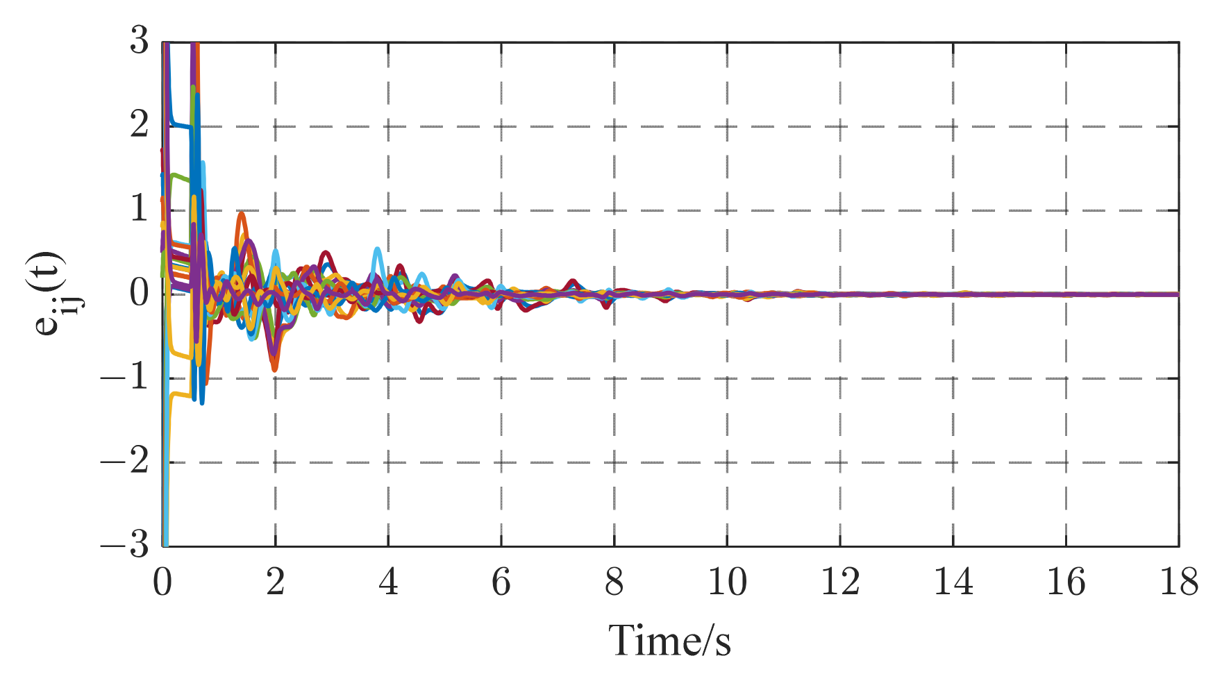
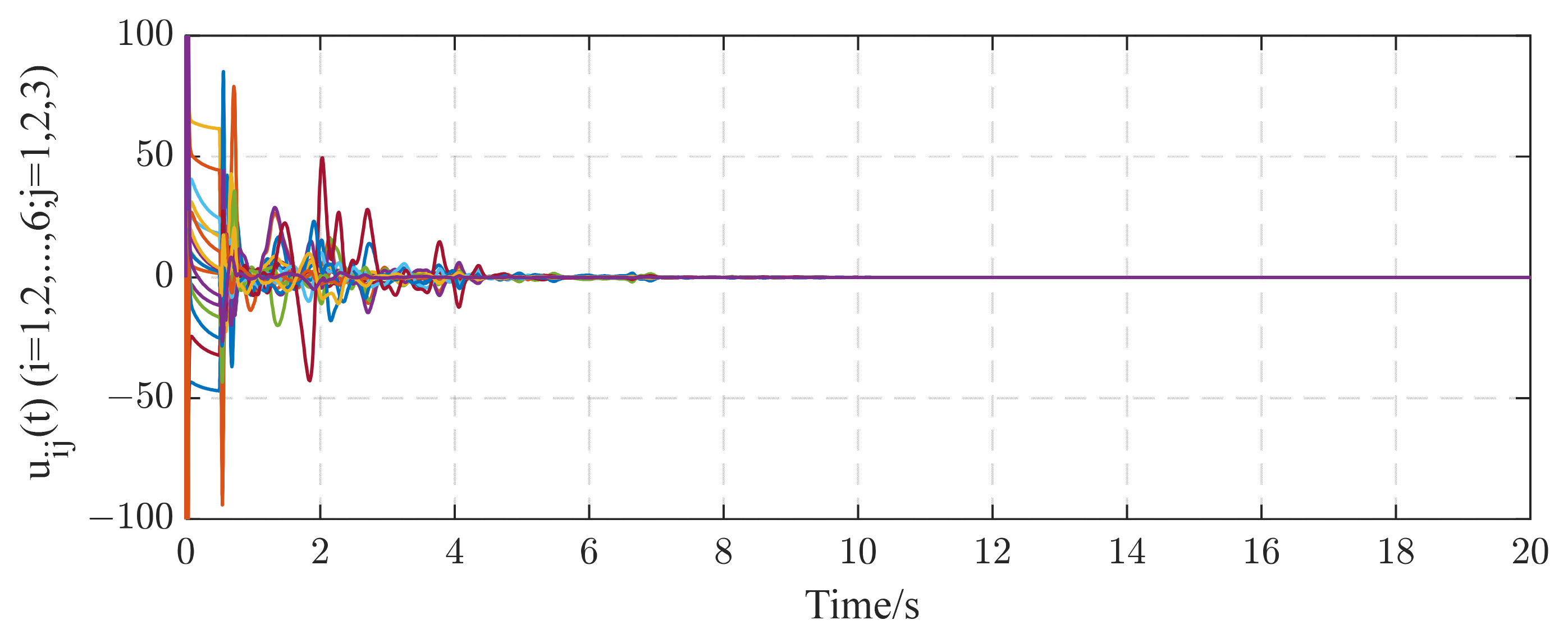
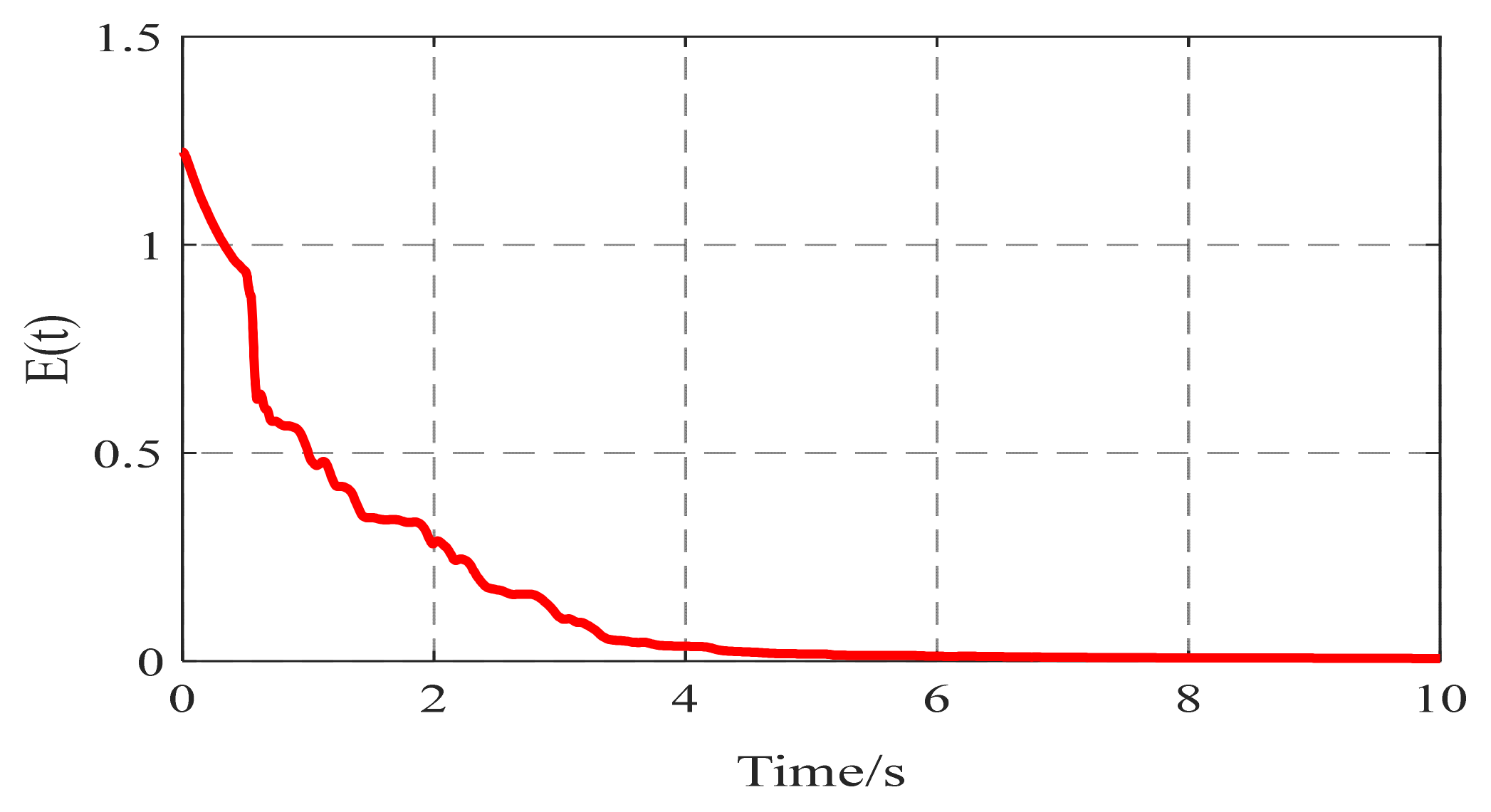
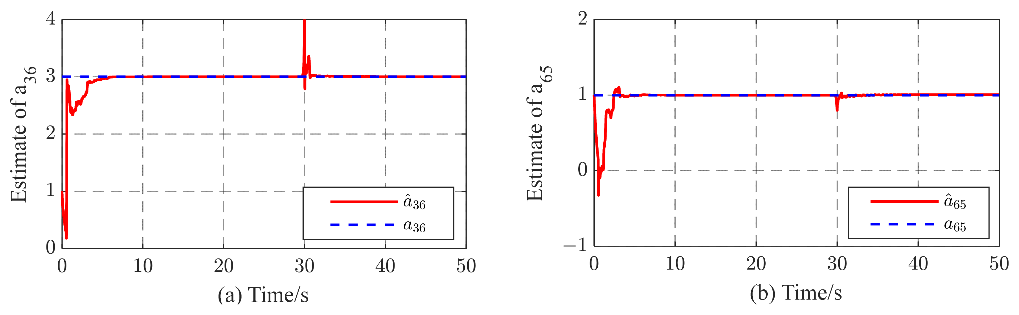
4.1.1. The Effectiveness of the Proposed STO

In this subsection, we consider a TICDN with fixed coupling strength. Without loss of generality, we assume that the coupling strength is $c=1$. Figure 2 and Figure 3 display the numerical results based on Equations (5)–(7). Figure 1 shows the temporal evolution of the synchronization errors (4). As time progresses, the synchronization errors gradually approach zero, indicating successful synchronization. Figure 2 displays the estimation of the six existing edges, $a_{12}$, $a_{23}$, $a_{36}$, $a_{46}$, $a_{52}$, $a_{65}$. These figures indicate that the topological parameter ${\widehat{a}}_{ij}$ can converge to the real valve of $a_{ij} (i,j=1,2\cdots ,6)$ by using the proposed STO. Figure 4 illustrates the temporal evolution of the effective control inputs $u_i(t)=[u_{i1}(t);u_{i2}(t);u_{i3}(t)] (i=1,2,\dots ,6)$ via Theorem 1.

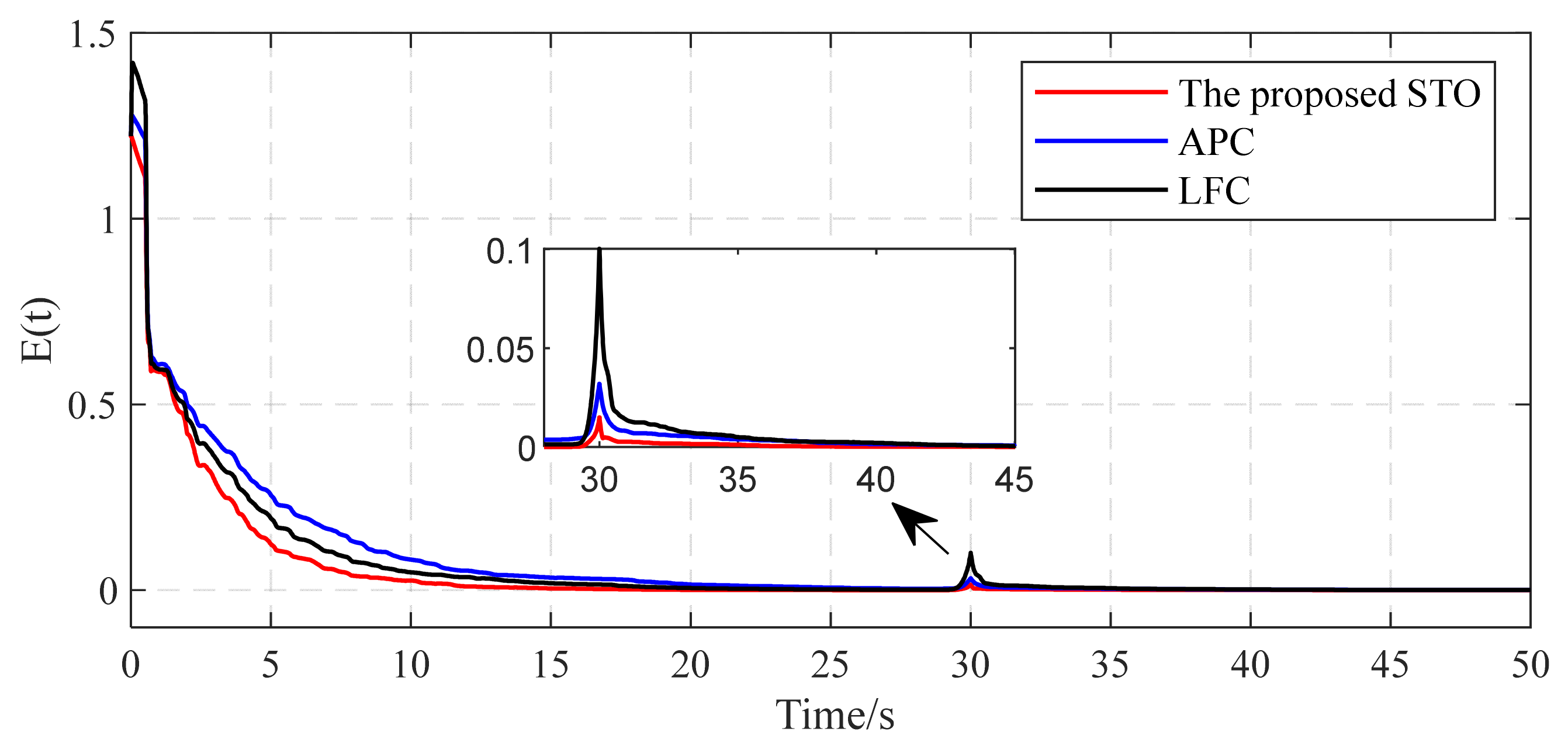
4.1.2. Comparison with Other Methods

In this part, the identification error of the proposed STO is also compared with two classical methods, including the observer-based adaptive pinning control (APC) in [22] and the observer-based linear feedback control (LFC) in [25]. The comparison methods have the same initial condition.

(i)

Performance indices

To facilitate quantitative comparison and analysis, the following three performance indices are given. Here, $T$ represents simulation time. The identification error is denoted as $E(t)$.

• Minimum identification time ($MIT$): the time needed for successful identification when $E(t)$ decreases to a specific value $\omega$. In this study, we adopt a $\omega$ value of $3\times {10}^{-3}$.
• The integral of the identification error ($IE$) is calculated as follows:

  $$IE={\displaystyle {\int }_0^{T}E(t)dt}$$

  where

  $$E(t)={\displaystyle \sum _{i=1}^N{\displaystyle \sum _{j=1}^N\left|{\widehat{a}}_{ij}-a_{ij}\right|}}/N^2$$
• The final error result of the identification topology is given by the steady-state error ($SE$):

  $$SE={\lim }_{t\to T}E(t)$$

(ii)

Identification results

Figure 5 shows the convergence process of identification errors using different methods. The relative performance indices in terms of $IE$, $SE$, and $MIT$ in

Table 1. Comparison of the performance indices with the different methods.

Method Indices	$\mathit{I}\mathit{E}$	$\mathit{S}\mathit{E}$	$\mathit{M}\mathit{I}\mathit{T}(\mathit{s})$
The proposed STO	2.5540 (65.77%) *	5.6230 × 10−5 (2.129%)	18.3301 (61.96%)
LFC [24]	3.8829 (100.0%)	2.6411 × 10−3 (100.0%)	29.5825 (100.0%)
APC [35]	3.2815 (84.50%)	1.1611 × 10−3 (43.96%)	22.8965 (77.39%)

* ($\zeta$) is the relative ratio. The chosen maximum value at each index is denoted as $\Delta$, with the definition of $\zeta =\frac{\mathsf{\Omega }}{\Delta }\times 100\%$ provided, where $\mathsf{\Omega }$ signifies the remaining value at each index.

are calculated based on the curves shown in Figure 5. As shown in Table 1, compared with the APC [22] and LFC [25] methods, the proposed STO has decreased performance index $IE$ by 34.32% and 18.73%, respectively. In addition, the proposed STO achieves the smallest steady-state identification error $SE$ among the three different methods. These results provide evidence that the proposed STO has better identification performance and higher accuracy than the others. Additionally, upon comparing the minimum identification times, the convergence speed of the proposed STO is obviously faster than others. The identification error is less than $3\times {10}^{-3}$, achieved with the shortest time of 18.33 s.

Considering the aforementioned discussion, it can be concluded that the proposed STO method outperforms the other two methods in terms of its smaller tracking error, faster convergence rate, and higher identification precision.

4.2. Identification Topology of Complex Networks with Adaptive Coupling Strength

In the last section, we discuss the effect of the proposed STO in solving a TICDN with a fixed coupling strength. However, in the real world, the coupling strength in complex networks may not be static, but instead, an adaptive parameter. The coupling strength is dynamically adjusted based on changes in the environment or the network itself (e.g., neural networks, wireless sensor networks, and social networks). In this section, we discuss the fact that the coupling strength of complex networks is adaptive during the identification process. The remaining initial arguments are the same as in Section 4.1. We take the initial value of $\widehat{\mathrm{\Theta }}(0)=2,\epsilon =0.01$.

Figure 6 shows the identification results of the six existing edge elements in the coupling matrix $A_{6*6}$, which converge to their real values as time increase. According to Figure 6, the identification error $E(t)$ tends to zero. Figure 6 and Figure 7 indicate that the unknown topology of complex networks are determined successfully by using controller (5) and update laws (6)–(8). Figure 8 shows the temporal evolution of the effective control inputs $u_i(t)=[u_{i1}(t);u_{i2}(t);u_{i3}(t)](i=1,2,\dots ,6)$.

Figure 9a shows the variation in $\widehat{\mathrm{\Theta }}(t)$ according to the adaptive law (15). Meanwhile, the coupling strength $c(t)$ adjusts itself to reach a certain constant value, as depicted in Figure 9b. In Figure 9, the topology of complex networks with adaptive coupling strength can be identified correctly and effectively, which aligns with the findings presented in Theorem 2.

4.3. Robustness Test for Topology Identification

4.3.1. Complex Networks with Fixed Coupling Strength

• Case 1: robustness to parameter variation

Generally speaking, it is necessary to consider robustness when designing an observer. In the process of parameter identification, one of the more common concerns is the problem of the robustness of the proposed STO, which is influenced by the variation in unknown topological parameters. In the real world, the connections between nodes may strengthen or weaken over time. Here, we assumed that a portion of the unknown topological parameter $a_{ij}$ is affected at a given time. Figure 10 shows the temporal evolution of ${\widehat{a}}_{36},{\widehat{a}}_{65}$ when $a_{36}=3,a_{65}=1$ turns to $a_{36}=1,a_{65}=2$ at $t=40 \mathrm{s}$. It is evident that all of the methods can automatically and accurately track over time. However, the proposed STO exhibits a noticeably faster convergence speed compared to the other methods. This indicates that the proposed STO possesses rapid tracking capabilities and strong robustness in the face of variations in topological parameters.

• Case 2: robustness to external disturbances

In order to prove the reliability of the proposed STO scheme, a robustness test is conducted on complex networks with external disturbances in this sub-part. Here, the external disturbances chosen are $s(t)=\sin (t)$$(28\le t\le 30)$. The coupling matrix $\Gamma$ is replaced with $\overline{\Gamma }={\left[\Gamma s(t)\right]}_{6\times 6}$.

Figure 11 shows topology identification error $E(t)$ curves under different methods. It is seen that the proposed STO exhibits stronger anti-disturbance capability. The estimations of all unknown topological parameters converge to their actual values within seconds. The performance indices in

Table 2. Comparison of performance indices with different methods.

Method Indices	$\mathit{I}\mathit{E}$	$\mathit{S}\mathit{E}$	$\mathit{M}\mathit{I}\mathit{T}(\mathit{s})$
The proposed STO	2.5776 (65.32%)	4.1985 × 10−6 (1.247%)	30.4419 (82.07%)
LFC [24]	3.9458 (100.0%)	3.3647 × 10−4 (100.0%)	37.0951 (100.0%)
ASC [35]	3.3868 (85.97%)	1.8896 × 10−4 (56.16%)	36.7364 (99.03%)

are calculated using the curves depicted in Figure 10. Upon comparing the identification performance indices, it is clear that the proposed STO shows its superiority across all performance indices when compared to the other two methods. From these simulation results, we can see that the proposed STO has better robustness capability, including a lower identification error and shorter convergence time, particularly in the presence of external disturbances affecting the complex networks.

4.3.2. Complex Networks with Adaptive Coupling Strength

To illustrate the robustness of the identification method to cases where the coupling strength is unknown, in our simulations, we also consider the uncertainties and external perturbations of complex networks. Figure 12 and Figure 13 show the simulation plots. From these simulations, it can be observed that the proposed method exhibits not only excellent tracking performance but also remarkable robustness against parametric variations and external disturbances. As illustrated in Figure 12, the proposed method demonstrates an ability to rapidly track changes in the unknown parameter while maintaining consistently good performance. In addition, as noted in Figure 13, the topological parameters ${\widehat{a}}_{36}$ and ${\widehat{a}}_{65}$ can recover the original defined values even after experiencing external disturbances. In addition, after $5~7 \mathrm{s},$ the state $y_i$$(i=1,2\dots ,6)$ quickly synchronizes with the state $x_i$.

5. Conclusions

In this paper, a novel synchronization-based topology observer for TICDNs is presented. Two kinds of network models are considered: online topology estimation of complex networks (i) with coupling delay and fixed coupling strength and (ii) with coupling delay and adaptive coupling strength. Based on the stability theorem approach, several useful estimation criteria for the real-time identification of topology weights are obtained. The identification method proposed is not only applied to complex delayed networks with fixed coupling strength, but is also suitable for complex delayed networks with adaptive coupling strength during the identification process. Simulation results are obtained to validate the effectiveness of the proposed STO using Theorems 1 and 2. The synchronization errors of the networks with fixed or adaptive coupling strength all tend to zero as time evolves in Figure 2 and Figure 7. The unknown topology can be successfully identified within seconds, as shown in Figure 3 and Figure 6. In other words, achieving synchronization ensures the correct identification of topological structures. Even though cases of external perturbations and parameter variation exist in complex networks, as shown in Figure 10 and Figure 13, the topological parameter identification results are still correct. In addition, under the same simulation time and the same identification error requirement, based on the computational indicators in Table 1 and Table 2, the proposed STO achieves high accuracy and stability. In addition, from an application point of view, the proposed method is capable of the automatic online adjustment of parameters, which may be easily implemented in practical applications. However, it would also be very interesting to study time-varying delays between the nodes, and we will further investigate this problem in the future.

References

1. Albert, R.; Barabasi, A.L. Statistical mechanics of complex networks. Rev. Mod. Phys. 2002, 26, 1–54. [Google Scholar] [CrossRef]
2. Ping, L.; Lam, J. Synchronization in networks of genetic oscillators with delayed coupling. Asian J. Control 2011, 13, 713–725. [Google Scholar]
3. Gu, H.; Liu, K.; Zhu, G.; Lü, J. Leader-following consensus of stochastic dynamical multi-agent systems with fixed and switching topologies under proportional-integral protocols. Asian J. Control 2023, 25, 662–676. [Google Scholar] [CrossRef]
4. Huang, W.; Liu, T.; Liu, H.; Huang, Y.; Chen, S. Robust consensus of heterogeneous multiagent systems with switching topologies: A time-delay case. Asian J. Control 2023, 25, 1336–1349. [Google Scholar] [CrossRef]
5. Baruch, I.S.; Quintana, V.A.; Reynaud, E.P. Complex-valued neural network topology and learning applied for identification and control of nonlinear systems. Neurocomputing 2017, 233, 104–115. [Google Scholar] [CrossRef]
6. Kazemy, A. Synchronization analysis of complex dynamical networks with hybrid coupling with application to Chua’s circuit. J. Control 2020, 14, 53–61. [Google Scholar] [CrossRef]
7. Dkhichi, F.; Oukarfi, B.; Fakkar, A.; Belbounaguia, N. Parameter identification of solar cell model using Levenberg–Marquardt algorithm combined with simulated annealing. Sol. Energy 2014, 110, 781–788. [Google Scholar] [CrossRef]
8. Peng, H.; Li, L.; Kurths, J.; Li, S.; Yang, Y. Topology Identification of Complex Network via Chaotic Ant Swarm Algorithm. Math. Probl. Eng. 2013, 2013, 401983. [Google Scholar] [CrossRef]
9. Wang, J.; Zhou, B.; Zhou, S. An improved cuckoo search optimization algorithm for the problem of chaotic systems pa-rameter estimation. Comput. Intel. Neurosci. 2016, 25, 2959370. [Google Scholar]
10. Tian, Z.; Wu, W.; Zhang, B. A Mixed Integer Quadratic Programming Model for Topology Identification in Distribution Network. IEEE Trans. Power Syst. 2016, 31, 823–824. [Google Scholar] [CrossRef]
11. Zhang, W.; Liu, W.; Zang, C.; Liu, L. Multiagent System-Based Integrated Solution for Topology Identification and State Estimation. IEEE Trans. Ind. Inform. 2017, 13, 714–724. [Google Scholar] [CrossRef]
12. Wei, Y.; Stanford, R.J. Parameter identification of solid oxide fuel cell by Chaotic Binary Shark Smell Optimization method. Energy 2019, 188, 115770. [Google Scholar] [CrossRef]
13. Li, G.; Wu, X.; Liu, J.; Lu, J.-A.; Guo, C. Recovering network topologies via Taylor expansion and compressive sensing. Chaos 2015, 25, 043102. [Google Scholar] [CrossRef] [PubMed]
14. Li, G.; Li, N.; Liu, S.; Wu, X. Compressive sensing-based topology identification of multilayer networks. Chaos 2019, 29, 053117. [Google Scholar] [CrossRef] [PubMed]
15. Babakmehr, M.; Simoes, M.G.; Wakin, M.B.; Harirchi, F. Compressive Sensing-Based Topology Identification for Smart Grids. IEEE Trans. Ind. Inform. 2016, 12, 532–543. [Google Scholar] [CrossRef]
16. Jahandari, S.; Materassi, D. Topology Identification of Dynamical Networks via Compressive Sensing. IFAC-PapersOnLine 2018, 51, 575–580. [Google Scholar] [CrossRef]
17. Wu, X.; Zhao, X.; Lu, J.; Tang, L.; Lu, J.-A. Identifying topologies of complex dynamical networks with stochastic perturbations. IEEE Trans. Control Netw. Syst. 2017, 3, 379–389. [Google Scholar] [CrossRef]
18. Lü, L.; Li, C.; Bai, S.; Li, G.; Rong, T.; Gao, Y.; Yan, Z. Synchronization of uncertain time-varying network based on sliding mode control technique. Physica A 2017, 482, 808–817. [Google Scholar] [CrossRef]
19. Behinfaraz, R.; Ghaemi, S.; Khanmohammadi, S.; Badamchizadeh, M.A. Time-varying parameters identification and synchronization of switching complex networks using the adaptive fuzzy-impulsive control with an application to secure communication. Asian J. Control 2022, 24, 377–387. [Google Scholar] [CrossRef]
20. Wang, X.; Gu, H.; Wang, Q.; Lü, J. Identifying topologies and system parameters of uncertain time-varying delayed complex networks. Sci. China Technol. Sci. 2019, 62, 94–105. [Google Scholar] [CrossRef]
21. Duan, W.; Du, B.; You, J.; Zou, Y. Synchronization criteria for neutral complex dynamic networks with internal time-vary coupling delays. Asian J. Control 2013, 15, 1385–1396. [Google Scholar] [CrossRef]
22. Xu, J.; Zhang, J.; Tang, W. Parameters and structure identification of complex delayed networks via pinning control. Trans. Inst. Meas. Control 2013, 35, 619–624. [Google Scholar] [CrossRef]
23. Chen, Z.; Yuan, X.; Yuan, Y.; Iu, H.H.-C.; Fernando, T. Parameter identification of chaotic and hyper-chaotic systems using synchronization-based parameter observer. IEEE Trans. Circuits Syst. I Regul. Pap. 2016, 63, 1464–1475. [Google Scholar] [CrossRef]
24. Zheng, Y.; Wu, X.; Fan, Z.; Wang, W. Identifying topology and system parameters of fractional-order complex dynamical networks. Appl. Math. Comput. 2022, 414, 126666. [Google Scholar] [CrossRef]
25. Xu, Y.; Zhou, W.; Zhang, J.; Sun, W.; Tong, D. Topology identification of complex delayed dynamical networks with multiple response systems. Nonlinear Dyn. 2017, 88, 2969–2981. [Google Scholar] [CrossRef]
26. Wang, F.X.; Zhang, J.; Shu, Y.J.; Liu, X.G. Stability analysis for fractional-order neural networks with time-varying delay. Asian J. Control 2023, 25, 1488–1498. [Google Scholar] [CrossRef]
27. Zhao, Y.; Li, X.; Duan, P. Observer-based sliding mode control for synchronization of delayed chaotic neural networks with unknown disturbance. Neural Netw. 2019, 117, 268–273. [Google Scholar] [CrossRef] [PubMed]
28. Zhang, W.; Li, H.; Li, C.; Li, Z.; Yang, X. Fixed-time synchronization criteria for complex networks via quantized pinning control. ISA Trans. 2019, 91, 151–156. [Google Scholar] [CrossRef] [PubMed]
29. Grzybowski, J.; Macau, E.; Yoneyama, T. The Lyapunov–Krasovskii theorem and a sufficient criterion for local stability of isochronal synchronization in networks of delay-coupled oscillators. Physica D 2017, 346, 28–36. [Google Scholar] [CrossRef]
30. Liu, X.; Chen, T. Synchronization of Complex Networks via Aperiodically Intermittent Pinning Control. IEEE Trans. Autom. Control 2015, 60, 3316–3321. [Google Scholar] [CrossRef]
31. Wang, S.; Zhang, Z.; Lin, C.; Chen, J. Fixed-time synchronization for complex-valued BAM neural networks with time-varying delays via pinning control and adaptive pinning control. Chaos Solitons Fractals 2021, 153, 111583. [Google Scholar] [CrossRef]
32. Xiang, L.Y.; Yu, Y.Y.; Zhu, J.W. Moment-based analysis of pinning synchronization in complex networks. Asian J. Control 2022, 24, 669–685. [Google Scholar] [CrossRef]
33. Zhu, S.; Zhou, J.; Lu, J.-A. Identifying partial topology of complex dynamical networks via a pinning mechanism. Chaos 2018, 28, 043108. [Google Scholar] [CrossRef] [PubMed]
34. Chen, C.; Zhou, J.; Qu, F.; Song, C.; Zhu, S. Identifying partial topology of complex networks with stochastic perturbations and time delay. Commun. Nonlinear Sci. Numer. Simul. 2022, 115, 106779. [Google Scholar] [CrossRef]
35. Yue, C.-X.; Wang, L.; Hu, X.; Tang, H.-A.; Duan, S. Pinning control for passivity and synchronization of coupled memristive reaction–diffusion neural networks with time-varying delay. Neurocomputing 2020, 381, 113–129. [Google Scholar] [CrossRef]
36. Zhang, C.; Wang, J.; Zhang, D.; Shao, X. Synchronization and tracking of multi-spacecraft formation attitude control using adaptive sliding mode. Asian J. Control 2019, 21, 832–846. [Google Scholar] [CrossRef]
37. Wu, H.Y.; Wang, L.; Zhao, L.H.; Wang, J.L. Topology identification of coupled neural networks with multiple weights. Neurocomputing 2021, 457, 254–264. [Google Scholar] [CrossRef]
38. Tan, F.; Zhou, L.; Lu, J.; Chu, Y.; Li, Y. Fixed-time outer synchronization under double-layered multiplex networks with hybrid links and time-varying delays via delayed feedback control. Asian J. Control 2022, 24, 137–148. [Google Scholar] [CrossRef]
39. Wu, D.; Zhu, S.; Luo, X.; Wu, L. Effects of adaptive coupling on stochastic resonance of small-world networks. Phys. Rev. E 2011, 84, 021102. [Google Scholar] [CrossRef] [PubMed]
40. Huang, D.; Fan, X.; Yu, Z.; Jiang, H. On Multitracking of First-Order MASs with Adaptive Coupling Strength. Discret. Dyn. Nat. Soc. 2020, 2020, 8897487. [Google Scholar] [CrossRef]
41. Wu, Y.; Li, Y.; Li, W. Synchronization of random coupling delayed complex networks with random and adaptive coupling strength. Nonlinear Dyn. 2019, 96, 2393–2412. [Google Scholar] [CrossRef]
Figure 1. Block diagram of topology identification based on synchronization.
Entropy 26 00525 g001
Figure 2. The temporal evolution of the synchronization error e i j ( i = 1 , 2 , , 6 ; j = 1 , 2 , 3 ) .
Entropy 26 00525 g002
Figure 3. Partial identification results (af) of network topology with the fixed coupling strength are displayed.
Entropy 26 00525 g003
Figure 4. The control inputs u i j ( t ) ( i = 1 , 2 , , 6 ; j = 1 , 2 , 3 ) under the networks with fixed coupling strength.
Entropy 26 00525 g004
Figure 5. Comparison of the identification error E ( t ) using different methods.
Entropy 26 00525 g005
Figure 6. Partial identification results (af) of network topology with adaptive coupling strength.
Entropy 26 00525 g006
Figure 7. The temporal evolution of the topology identification error E ( t ) .
Entropy 26 00525 g007
Figure 8. The control inputs u i j ( t ) ( i = 1 , 2 , , 6 ; j = 1 , 2 , 3 ) under the networks with adaptive coupling strength.
Entropy 26 00525 g008
Figure 9. The temporal evolution of (a) Θ ^ ( t ) and (b) adaptive coupling strength c ( t ) .
Entropy 26 00525 g009
Figure 10. Identification results of (a) a ^ 36 and (b) a ^ 65 .
Entropy 26 00525 g010
Figure 11. Comparison of identification error E ( t ) with external disturbances.
Entropy 26 00525 g011
Figure 12. Tracking results while a 36 = 3 , a 65 = 1 turns to a 36 = 1 , a 65 = 2 at t =   s ; (a,b) temporal evolution of a ^ 36 , a ^ 65 , respectively.
Entropy 26 00525 g012
Figure 13. (a,b) Temporal evolution of estimates a ^ 36 , a ^ 65 , respectively, in complex dynamic network with external disturbances at t =   s .
Entropy 26 00525 g013