
Partial Information Decomposition: Redundancy as Information Bottleneck


Abstract
1. Introduction
2. Background
2.1. Information Bottleneck (IB)
2.2. Partial Information Decomposition
2.3. Blackwell Redundancy
3. Redundancy Bottleneck
3.1. Reformulation of Blackwell Redundancy
3.2. Redundancy Bottleneck
3.3. Contributions from Different Sources
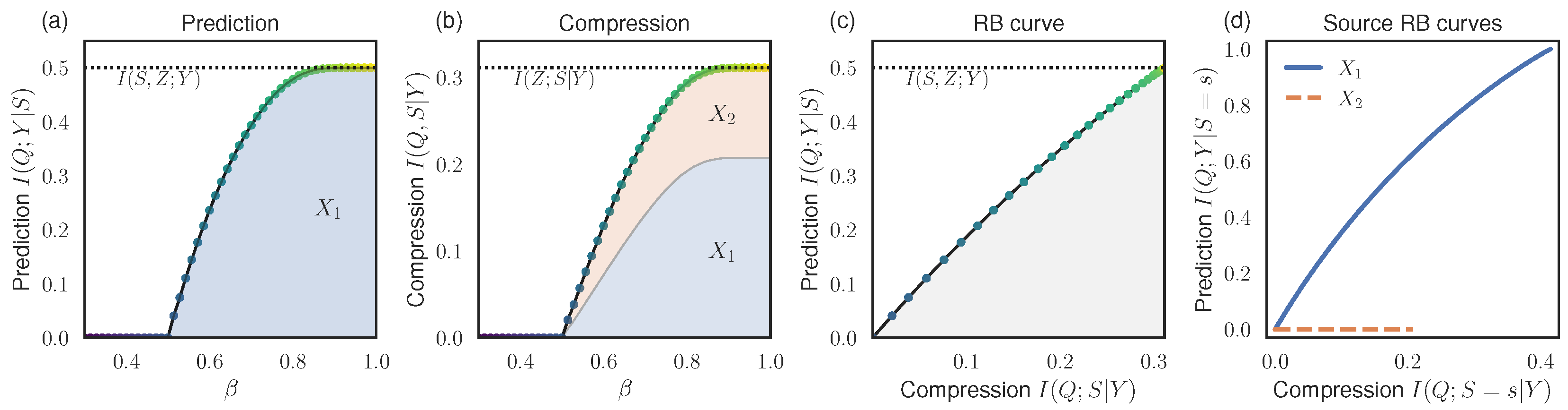
3.4. Examples
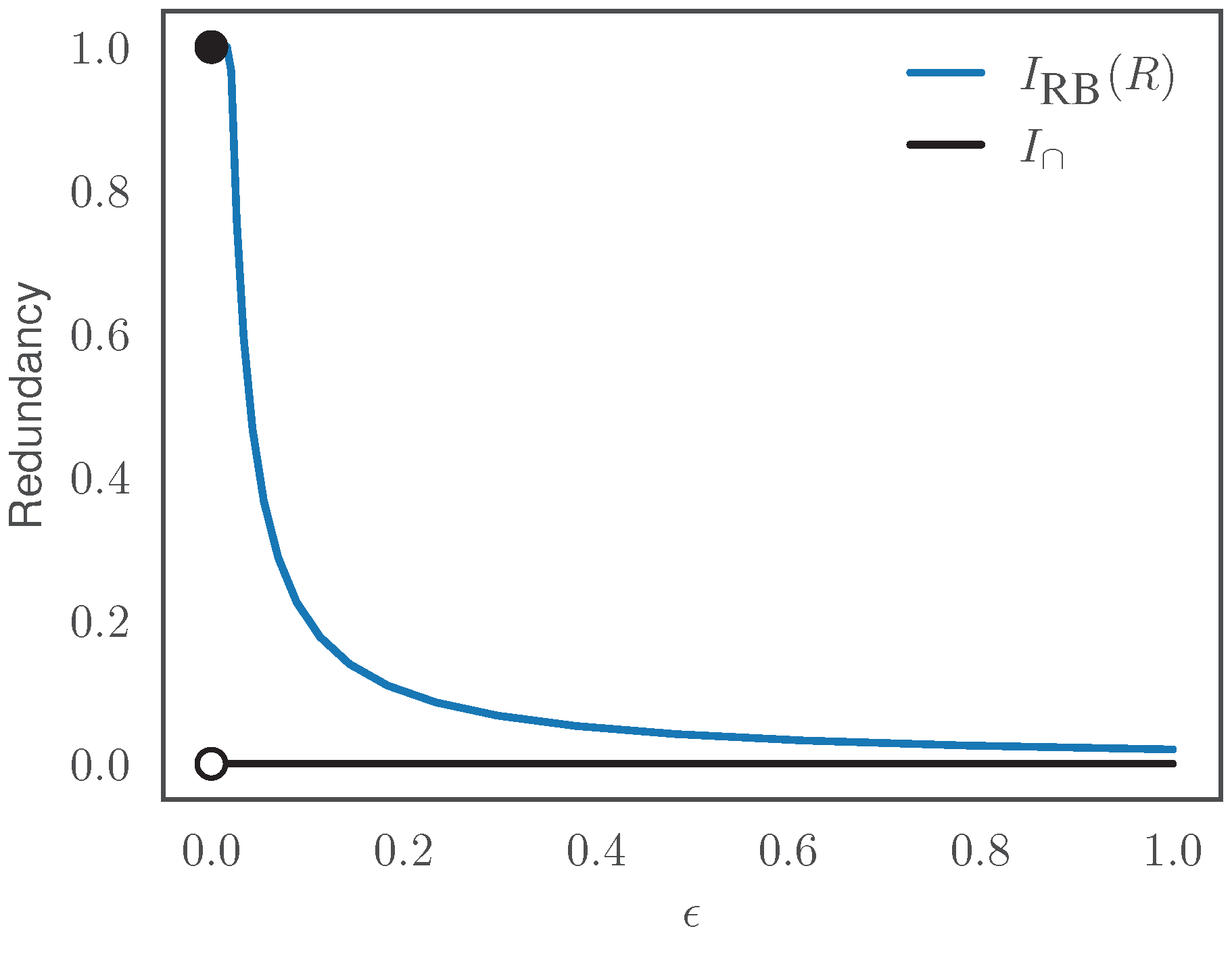
3.5. Continuity
4. Iterative Algorithm
5. Discussion
Funding
Institutional Review Board Statement
Informed Consent Statement
Data Availability Statement
Acknowledgments
Conflicts of Interest
Appendix A
Appendix A.1. Proof of Theorem 1
Appendix A.2. Proof of Theorem 2
Appendix A.3. Proof of Theorem 3
Appendix A.4. Proof of Theorem 4
References
- Williams, P.L.; Beer, R.D. Nonnegative decomposition of multivariate information. arXiv 2010, arXiv:1004.2515. [Google Scholar]
- Wibral, M.; Priesemann, V.; Kay, J.W.; Lizier, J.T.; Phillips, W.A. Partial information decomposition as a unified approach to the specification of neural goal functions. Brain Cogn. 2017, 112, 25–38. [Google Scholar] [CrossRef] [PubMed]
- Lizier, J.; Bertschinger, N.; Jost, J.; Wibral, M. Information decomposition of target effects from multi-source interactions: Perspectives on previous, current and future work. Entropy 2018, 20, 307. [Google Scholar] [CrossRef] [PubMed]
- Kolchinsky, A. A Novel Approach to the Partial Information Decomposition. Entropy 2022, 24, 403. [Google Scholar] [CrossRef]
- Williams, P.L. Information Dynamics: Its Theory and Application to Embodied Cognitive Systems. Ph.D. Thesis, Indiana University, Bloomington, IN, USA, 2011. [Google Scholar]
- Tishby, N.; Pereira, F.; Bialek, W. The information bottleneck method. In Proceedings of the 37th Allerton Conference on Communication, Monticello, IL, USA, 22–24 September 1999. [Google Scholar]
- Hu, S.; Lou, Z.; Yan, X.; Ye, Y. A Survey on Information Bottleneck. IEEE Trans. Pattern Anal. Mach. Intell. 2024, 1–20. [Google Scholar] [CrossRef] [PubMed]
- Palmer, S.E.; Marre, O.; Berry, M.J.; Bialek, W. Predictive information in a sensory population. Proc. Natl. Acad. Sci. USA 2015, 112, 6908–6913. [Google Scholar] [CrossRef]
- Wang, Y.; Ribeiro, J.M.L.; Tiwary, P. Past–future information bottleneck for sampling molecular reaction coordinate simultaneously with thermodynamics and kinetics. Nat. Commun. 2019, 10, 3573. [Google Scholar] [CrossRef] [PubMed]
- Zaslavsky, N.; Kemp, C.; Regier, T.; Tishby, N. Efficient compression in color naming and its evolution. Proc. Natl. Acad. Sci. USA 2018, 115, 7937–7942. [Google Scholar] [CrossRef] [PubMed]
- Alemi, A.A.; Fischer, I.; Dillon, J.V.; Murphy, K. Deep variational information bottleneck. In Proceedings of the International Conference on Learning Representations (ICLR), Toulon, France, 24–26 April 2017; Available online: https://openreview.net/forum?id=HyxQzBceg (accessed on 12 May 2024).
- Kolchinsky, A.; Tracey, B.D.; Wolpert, D.H. Nonlinear information bottleneck. Entropy 2019, 21, 1181. [Google Scholar] [CrossRef]
- Fischer, I. The conditional entropy bottleneck. Entropy 2020, 22, 999. [Google Scholar] [CrossRef]
- Goldfeld, Z.; Polyanskiy, Y. The information bottleneck problem and its applications in machine learning. IEEE J. Sel. Areas Inf. Theory 2020, 1, 19–38. [Google Scholar] [CrossRef]
- Ahlswede, R.; Körner, J. Source Coding with Side Information and a Converse for Degraded Broadcast Channels. IEEE Trans. Inf. Theory 1975, 21, 629–637. [Google Scholar] [CrossRef]
- Witsenhausen, H.; Wyner, A. A conditional entropy bound for a pair of discrete random variables. IEEE Trans. Inf. Theory 1975, 21, 493–501. [Google Scholar] [CrossRef]
- Gilad-Bachrach, R.; Navot, A.; Tishby, N. An Information Theoretic Tradeoff between Complexity and Accuracy. In Learning Theory and Kernel Machines; Goos, G., Hartmanis, J., van Leeuwen, J., Schölkopf, B., Warmuth, M.K., Eds.; Springer: Berlin/Heidelberg, Germany, 2003; Volume 2777, pp. 595–609. [Google Scholar] [CrossRef]
- Kolchinsky, A.; Tracey, B.D.; Van Kuyk, S. Caveats for information bottleneck in deterministic scenarios. In Proceedings of the International Conference on Learning Representations (ICLR), New Orleans, LA, USA, 6–9 May 2019; Available online: https://openreview.net/forum?id=rke4HiAcY7 (accessed on 12 May 2024).
- Rodríguez Gálvez, B.; Thobaben, R.; Skoglund, M. The convex information bottleneck lagrangian. Entropy 2020, 22, 98. [Google Scholar] [CrossRef] [PubMed]
- Benger, E.; Asoodeh, S.; Chen, J. The cardinality bound on the information bottleneck representations is tight. In Proceedings of the 2023 IEEE International Symposium on Information Theory (ISIT), Taipei, Taiwan, 25–30 June 2023; pp. 1478–1483. [Google Scholar]
- Geiger, B.C.; Fischer, I.S. A comparison of variational bounds for the information bottleneck functional. Entropy 2020, 22, 1229. [Google Scholar] [CrossRef] [PubMed]
- Federici, M.; Dutta, A.; Forré, P.; Kushman, N.; Akata, Z. Learning robust representations via multi-view information bottleneck. arXiv 2020, arXiv:2002.07017. [Google Scholar]
- Murphy, K.A.; Bassett, D.S. Machine-Learning Optimized Measurements of Chaotic Dynamical Systems via the Information Bottleneck. Phys. Rev. Lett. 2024, 132, 197201. [Google Scholar] [CrossRef] [PubMed]
- Slonim, N.; Friedman, N.; Tishby, N. Multivariate Information Bottleneck. Neural Comput. 2006, 18, 1739–1789. [Google Scholar] [CrossRef]
- Shannon, C. The lattice theory of information. Trans. IRE Prof. Group Inf. Theory 1953, 1, 105–107. [Google Scholar] [CrossRef]
- McGill, W. Multivariate information transmission. Trans. IRE Prof. Group Inf. Theory 1954, 4, 93–111. [Google Scholar] [CrossRef]
- Reza, F.M. An Introduction to Information Theory; Dover Publications: Mineola, NY, USA, 1961. [Google Scholar]
- Ting, H.K. On the amount of information. Theory Probab. Its Appl. 1962, 7, 439–447. [Google Scholar] [CrossRef]
- Han, T. Linear dependence structure of the entropy space. Inf. Control 1975, 29, 337–368. [Google Scholar] [CrossRef]
- Yeung, R.W. A new outlook on Shannon’s information measures. IEEE Trans. Inf. Theory 1991, 37, 466–474. [Google Scholar] [CrossRef]
- Bell, A.J. The co-information lattice. In Proceedings of the Fifth International Workshop on Independent Component Analysis and Blind Signal Separation: ICA, Nara, Japan, 1–4 April 2003; Volume 2003. [Google Scholar]
- Gomes, A.F.; Figueiredo, M.A. Orders between Channels and Implications for Partial Information Decomposition. Entropy 2023, 25, 975. [Google Scholar] [CrossRef] [PubMed]
- Griffith, V.; Koch, C. Quantifying synergistic mutual information. In Guided Self-Organization: Inception; Springer Berlin/Heidelberg, Germany, 2014; pp. 159–190.
- Griffith, V.; Chong, E.K.; James, R.G.; Ellison, C.J.; Crutchfield, J.P. Intersection information based on common randomness. Entropy 2014, 16, 1985–2000. [Google Scholar] [CrossRef]
- Griffith, V.; Ho, T. Quantifying redundant information in predicting a target random variable. Entropy 2015, 17, 4644–4653. [Google Scholar] [CrossRef]
- Bertschinger, N.; Rauh, J. The Blackwell relation defines no lattice. In Proceedings of the 2014 IEEE International Symposium on Information Theory, Honolulu, HI, USA, 29 June–4 July 2014; pp. 2479–2483. [Google Scholar]
- Blackwell, D. Equivalent comparisons of experiments. Ann. Math. Stat. 1953, 24, 265–272. [Google Scholar] [CrossRef]
- Rauh, J.; Banerjee, P.K.; Olbrich, E.; Jost, J.; Bertschinger, N.; Wolpert, D. Coarse-Graining and the Blackwell Order. Entropy 2017, 19, 527. [Google Scholar] [CrossRef]
- Bertschinger, N.; Rauh, J.; Olbrich, E.; Jost, J.; Ay, N. Quantifying unique information. Entropy 2014, 16, 2161–2183. [Google Scholar] [CrossRef]
- Rauh, J.; Banerjee, P.K.; Olbrich, E.; Jost, J.; Bertschinger, N. On extractable shared information. Entropy 2017, 19, 328. [Google Scholar] [CrossRef]
- Venkatesh, P.; Schamberg, G. Partial information decomposition via deficiency for multivariate gaussians. In Proceedings of the 2022 IEEE International Symposium on Information Theory (ISIT), Espoo, Finland, 26 June–1 July 2022; pp. 2892–2897. [Google Scholar]
- Mages, T.; Anastasiadi, E.; Rohner, C. Non-Negative Decomposition of Multivariate Information: From Minimum to Blackwell Specific Information. Entropy 2024, 26, 424. [Google Scholar] [CrossRef]
- Le Cam, L. Sufficiency and approximate sufficiency. Ann. Math. Stat. 1964, 35, 1419–1455. [Google Scholar] [CrossRef]
- Raginsky, M. Shannon meets Blackwell and Le Cam: Channels, codes, and statistical experiments. In Proceedings of the 2011 IEEE International Symposium on Information Theory, St. Petersburg, Russia, 31 July–5 August 2011; pp. 1220–1224. [Google Scholar]
- Banerjee, P.K.; Olbrich, E.; Jost, J.; Rauh, J. Unique informations and deficiencies. In Proceedings of the 2018 56th Annual Allerton Conference on Communication, Control, and Computing (Allerton), Monticello, IL, USA, 2–5 October 2018; pp. 32–38. [Google Scholar]
- Banerjee, P.K.; Montufar, G. The Variational Deficiency Bottleneck. In Proceedings of the 2020 International Joint Conference on Neural Networks (IJCNN), Glasgow, UK, 19–24 July 2020; pp. 1–8. [Google Scholar] [CrossRef]
- Venkatesh, P.; Gurushankar, K.; Schamberg, G. Capturing and Interpreting Unique Information. In Proceedings of the 2023 IEEE International Symposium on Information Theory (ISIT), Taipei, Taiwan, 25–30 June 2023; pp. 2631–2636. [Google Scholar] [CrossRef]
- Csiszár, I.; Matus, F. Information projections revisited. IEEE Trans. Inf. Theory 2003, 49, 1474–1490. [Google Scholar] [CrossRef]
- Makhdoumi, A.; Salamatian, S.; Fawaz, N.; Médard, M. From the information bottleneck to the privacy funnel. In Proceedings of the 2014 IEEE Information Theory Workshop (ITW 2014), Hobart, Australia, 2–5 November 2014; pp. 501–505. [Google Scholar]
- Janzing, D.; Balduzzi, D.; Grosse-Wentrup, M.; Schölkopf, B. Quantifying causal influences. Ann. Stat. 2013, 41, 2324–2358. [Google Scholar] [CrossRef]
- Ay, N. Confounding ghost channels and causality: A new approach to causal information flows. Vietnam. J. Math. 2021, 49, 547–576. [Google Scholar] [CrossRef]
- Kolchinsky, A.; Rocha, L.M. Prediction and modularity in dynamical systems. In Proceedings of the European Conference on Artificial Life (ECAL), Paris, France, 8–12 August 2011; Available online: https://direct.mit.edu/isal/proceedings/ecal2011/23/65/111139 (accessed on 12 May 2024).
- Hidaka, S.; Oizumi, M. Fast and exact search for the partition with minimal information loss. PLoS ONE 2018, 13, e0201126. [Google Scholar] [CrossRef] [PubMed]
- Rosas, F.; Ntranos, V.; Ellison, C.J.; Pollin, S.; Verhelst, M. Understanding interdependency through complex information sharing. Entropy 2016, 18, 38. [Google Scholar] [CrossRef]
- Rosas, F.E.; Mediano, P.A.; Gastpar, M.; Jensen, H.J. Quantifying high-order interdependencies via multivariate extensions of the mutual information. Phys. Rev. E 2019, 100, 032305. [Google Scholar] [CrossRef]
- Dubins, L.E. On extreme points of convex sets. J. Math. Anal. Appl. 1962, 5, 237–244. [Google Scholar] [CrossRef]
- Cover, T.M.; Thomas, J.A. Elements of Information Theory; John Wiley & Sons: Hoboken, NJ, USA, 2006. [Google Scholar]
- Timo, R.; Grant, A.; Kramer, G. Lossy broadcasting with complementary side information. IEEE Trans. Inf. Theory 2012, 59, 104–131. [Google Scholar] [CrossRef]


Disclaimer/Publisher’s Note: The statements, opinions and data contained in all publications are solely those of the individual author(s) and contributor(s) and not of MDPI and/or the editor(s). MDPI and/or the editor(s) disclaim responsibility for any injury to people or property resulting from any ideas, methods, instructions or products referred to in the content. |
© 2024 by the author. Licensee MDPI, Basel, Switzerland. This article is an open access article distributed under the terms and conditions of the Creative Commons Attribution (CC BY) license (https://creativecommons.org/licenses/by/4.0/).
Share and Cite
Kolchinsky, A. Partial Information Decomposition: Redundancy as Information Bottleneck. Entropy 2024, 26, 546. https://doi.org/10.3390/e26070546
Kolchinsky A. Partial Information Decomposition: Redundancy as Information Bottleneck. Entropy. 2024; 26(7):546. https://doi.org/10.3390/e26070546
Chicago/Turabian StyleKolchinsky, Artemy. 2024. "Partial Information Decomposition: Redundancy as Information Bottleneck" Entropy 26, no. 7: 546. https://doi.org/10.3390/e26070546
APA StyleKolchinsky, A. (2024). Partial Information Decomposition: Redundancy as Information Bottleneck. Entropy, 26(7), 546. https://doi.org/10.3390/e26070546