Optimum Achievable Rates in Two Random Number Generation Problems with f-Divergences Using Smooth Rényi Entropy ^†

Abstract

Two typical fixed-length random number generation problems in information theory are considered for general sources. One is the source resolvability problem and the other is the intrinsic randomness problem. In each of these problems, the optimum achievable rate with respect to the given approximation measure is one of our main concerns and has been characterized using two different information quantities: the information spectrum and the smooth Rényi entropy. Recently, optimum achievable rates with respect to f-divergences have been characterized using the information spectrum quantity. The f-divergence is a general non-negative measure between two probability distributions on the basis of a convex function f. The class of f-divergences includes several important measures such as the variational distance, the KL divergence, the Hellinger distance and so on. Hence, it is meaningful to consider the random number generation problems with respect to f-divergences. However, optimum achievable rates with respect to f-divergences using the smooth Rényi entropy have not been clarified yet in both problems. In this paper, we try to analyze the optimum achievable rates using the smooth Rényi entropy and to extend the class of f-divergence. To do so, we first derive general formulas of the first-order optimum achievable rates with respect to f-divergences in both problems under the same conditions as imposed by previous studies. Next, we relax the conditions on f-divergence and generalize the obtained general formulas. Then, we particularize our general formulas to several specified functions f. As a result, we reveal that it is easy to derive optimum achievable rates for several important measures from our general formulas. Furthermore, a kind of duality between the resolvability and the intrinsic randomness is revealed in terms of the smooth Rényi entropy. Second-order optimum achievable rates and optimistic achievable rates are also investigated.

1. Introduction

Two typical fixed-length random number generation problems in information theory are considered for general sources. One is the source resolvability problem (i.e., the resolvability problem), and the other is the intrinsic randomness problem. The problem setting of the resolvability problem is as follows. Given an arbitrary source $\mathbf{X}={\left\{X^n\right\}}_{n=1}^{\infty }$ (the target random number), we approximate it by using a discrete random number that is uniformly distributed, which we call the uniform random number. Here, the size of the uniform random number is requested to be as small as possible. In this setting, a degree of approximation is measured by several criteria. Han and Verdú [1] and Steinberg and Verdú [2] have determined the first-order optimum achievable rates with respect to the variational distance and the normalized Kullback–Leibler (KL) divergence. Nomura [3] has studied the first-order optimum achievable rates with respect to the KL divergence. Recently, Nomura [4] has characterized the first-order optimum achievable rates with respect to f-divergences. The class of f-divergence considered in [4] includes the variational distance and the KL divergence. Hence, the result can be considered as a generalization of the results given in [1,3]. The second-order optimum achievable rates in the resolvability problem have also been studied with respect to several approximation measures [4,5]. It should be noted that the results mentioned above are based on the information spectrum quantity. On the other hand, Uyematsu [6] has characterized the first-order optimum achievable rate with respect to the variational distance using the smooth Rényi entropy.

The intrinsic randomness problem, which is also one of typical random number generation problems, has also been studied. The problem setting of the intrinsic randomness problem is as follows. By using a given arbitrary source $\mathbf{X}={\left\{X^n\right\}}_{n=1}^{\infty }$ (the coin random number), we approximate a discrete uniform random number whose size is requested to be as large as possible. Also in the intrinsic randomness problem, optimum achievable rates with respect to various criteria have been considered. Vembu and Verdú [7] have considered the intrinsic randomness problem with respect to the variational distance as well as the normalized KL divergence and derived general formulas of the first-order optimum achievable rates (cf. Han [8]). Hayashi [9] has considered the first- and second-order optimum achievable rates with respect to the KL divergence. Recently, the first- and second-order optimum achievable rates with respect to f-divergences have been clarified in [4]. The results mentioned here are based on information spectrum quantities. On the other hand, Uyematsu and Kunimatsu [10] have characterized the first-order optimum achievable rates with respect to the variational distance using the smooth Rényi entropy.

Related works include works given by Liu, Cuff and Verdú [11], Yagi and Han [12], Kumagai and Hayashi [13,14], and Yu and Tan [15]. In [11], the channel resolvability problem with respect to the $E_{\gamma }$-divergence has been considered. They have applied their results to the case of the source resolvability problem. Yagi and Han [16] have determined the optimum variable-length resolvability rates with respect to the variational distance as well as the KL divergence. Kumagai and Hayashi [13,14] have determined the first- and second-order optimum achievable rates in the random number conversion problem. It should be noted that the random number conversion problem includes the resolvability and intrinsic randomness problems treated in this paper. In [13,14], an approximation measure related to the Hellinger distance has been used. Yu and Tan [15] have considered the random number conversion problem with respect to the Rényi divergence.

As we have mentioned above, in both problems of the resolvability and the intrinsic randomness, various approximation measures have been considered. Furthermore, general formulas of achievable rates have been characterized by using the information spectrum quantity and the smooth Rényi entropy. We here note that optimum achievable rates with respect to f-divergence using the smooth Rényi entropy have not been clarified yet. The smooth Rényi entropy is an information quantity that has a clear operational meaning and is easy to understand. Moreover, a class of f-divergences is a general distance measure, in which several important measures are included. In this paper, hence, we try to characterize the first- and second-order optimum achievable rates with respect to f-divergences using the smooth Rényi entropy. In addition, we also extend the class of f-divergence for which optimum achievable rates can be characterized. As a result, we find that two types of smooth Rényi entropies are useful to describe these optimum achievable rates for a wider class of f-divergence. Furthermore, a kind of duality between the resolvability and the intrinsic randomness is revealed in terms of the smooth Rényi entropy and f-divergences.

This paper is organized as follows. In Section 2, we describe the problem setting and give some definitions of the optimum first-order achievable rates. The class of f-divergences and the smooth Rényi entropy are also introduced. In Section 3 and Section 4, we show general formulas of the optimum first-order achievable rates in the resolvability problem and the intrinsic randomness problem, respectively. In Section 5, we derive the general formulas of these achievable rates for an extended class of f-divergence. In Section 6, we apply general formulas obtained in previous sections to some specified functions f and compute the optimum first-order achievable rates in each cases. In Section 7, we show general formulas of the optimum second-order achievable rates in two problems. In Section 8, optimum achievable rates in the optimistic sense are considered. Section 9 is devoted to the discussion concerning our results. Finally, we provide some concluding remarks on our results in Section 10.

2. Preliminaries

2.1. f-Divergences

The f-divergence between two probability distributions $P_Z$ and $P_{\overline{Z}}$ is defined as follows [17]. Let $f\left(t\right)$ be a convex function defined for $t>0$ and $f\left(1\right)=0$.

Definition 1 

(f-divergence [17]). Let $P_Z$ and $P_{\overline{Z}}$ denote probability distributions over a finite or countably infinite set $\mathcal{Z}$. The f-divergence between $P_Z$ and $P_{\overline{Z}}$ is defined by

$$D_f\left(Z\right||\overline{Z}):=\sum _{z\in \mathcal{Z}}{P}_{\overline{Z}}\left(z\right)f\left({\displaystyle \frac{P_Z\left(z\right)}{P_{\overline{Z}}\left(z\right)}}\right),$$

(1)

where we set $0f\left({\displaystyle \frac{0}{0}}\right)=0$, $f\left(0\right)={lim}_{t\downarrow 0}f\left(t\right)$, $0f\left({\displaystyle \frac{a}{0}}\right)={lim}_{t\to 0}tf\left({\displaystyle \frac{a}{t}}\right)=a{lim}_{u\to \infty }{\displaystyle \frac{f\left(u\right)}{u}}$.

The f-divergence is a general approximation measure, which includes some important measures. We give some examples of f-divergences [17,18]:

• $f\left(t\right)=tlogt$: (Kullback–Leibler (KL) divergence)

  $$\begin{array}{c}\hfill D_f\left(Z\right||\overline{Z})=\sum _{z\in \mathcal{Z}}{P}_Z\left(z\right)log{\displaystyle \frac{P_Z\left(z\right)}{P_{\overline{Z}}\left(z\right)}}=:D\left(Z\right||\overline{Z}).\end{array}$$

  (2)
• $f\left(t\right)=-logt$: (Reverse Kullback–Leibler divergence)

  $$\begin{array}{c}\hfill D_f\left(Z\right||\overline{Z})=\sum _{z\in \mathcal{Z}}{P}_{\overline{Z}}\left(z\right)log{\displaystyle \frac{P_{\overline{Z}}\left(z\right)}{P_Z\left(z\right)}}=D(\overline{Z}\left|\right|Z).\end{array}$$

  (3)
• $f\left(t\right)=1-\sqrt{t}$: (Hellinger distance)

  $$\begin{array}{c}\hfill D_f\left(Z\right||\overline{Z})=1-\sum _{z\in \mathcal{Z}}\sqrt{P_Z\left(z\right)P_{\overline{Z}}\left(z\right)}.\end{array}$$

  (4)
• $f\left(t\right)={(1-\sqrt{t})}^2$: (Squared Hellinger distance)

  $$\begin{array}{c}\hfill D_f\left(Z\right||\overline{Z})=\sum _{z\in \mathcal{Z}}{\left(\sqrt{P_Z\left(z\right)}-\sqrt{P_{\overline{Z}}\left(z\right)}\right)}^2.\end{array}$$

  (5)
• $f\left(t\right)=|t-1|$: (Variational distance)

  $$\begin{array}{c}\hfill D_f\left(Z\right||\overline{Z})=\sum _{z\in \mathcal{Z}}|P_Z\left(z\right)-P_{\overline{Z}}\left(z\right)|.\end{array}$$

  (6)
• $f\left(t\right)={(1-t)}^{+}:=max\{1-t,0\}$: (Half variational distance)

  $$\begin{array}{ccc}\hfill D_f\left(Z\right||\overline{Z})& =& {\displaystyle \frac{1}{2}}\sum _{z\in \mathcal{Z}}|P_Z\left(z\right)-P_{\overline{Z}}\left(z\right)|\hfill \\ & =& \sum _{z\in \mathcal{Z}:P_Z\left(z\right)>P_{\overline{Z}}\left(z\right)}\left(P_Z\left(z\right)-P_{\overline{Z}}\left(z\right)\right).\hfill \end{array}$$

  (7)
• $f\left(t\right)={\displaystyle \frac{t^{\alpha }-\alpha t-(1-\alpha )}{\alpha (\alpha -1)}}$: $\alpha$-divergence ($0<\alpha <1$)

  $$\begin{array}{ccc}\hfill D_f\left(Z\right||\overline{Z})& =& {\displaystyle \frac{1}{\alpha (\alpha -1)}}\left(1-\sum _{z\in \mathcal{Z}}{P}_Z{\left(z\right)}^{\alpha }{P}_{\overline{Z}}{\left(z\right)}^{1-\alpha }\right).\hfill \end{array}$$

  (8)
• $f\left(t\right)={(t-\gamma )}^{+}$ : ($E_{\gamma }$-divergence) For any given $\gamma \ge 1$,

  $$\begin{array}{c}\hfill D_f\left(Z\right||\overline{Z})=\sum _{z\in \mathcal{Z}:P_Z\left(z\right)>\gamma P_{\overline{Z}}\left(z\right)}\left(P_Z\left(z\right)-\gamma P_{\overline{Z}}\left(z\right)\right)=:E_{\gamma }\left(Z\right||\overline{Z}).\end{array}$$

  (9)

The $E_{\gamma }$-divergence is a generalization of the half variational distance defined in (7), because $\gamma \ge 1$ is arbitrary.

Remark 1. 

It is known [4] that the $E_{\gamma }$-divergence can be expressed as an f-divergence using the function:

$$f\left(t\right)={(\gamma -t)}^{+}+1-\gamma .$$

(10)

The following key property holds for the f-divergence from Jensen’s inequality [17]:

$$\begin{array}{ccc}\hfill \sum _{z\in {\mathcal{Z}}^{\prime }}b\left(z\right)f\left({\displaystyle \frac{a\left(z\right)}{b\left(z\right)}}\right)& \ge & \left(\sum _{z\in {\mathcal{Z}}^{\prime }}b\left(z\right)\right)f\left({\displaystyle \frac{{\sum }_{z\in {\mathcal{Z}}^{\prime }}a\left(z\right)}{{\sum }_{z\in {\mathcal{Z}}^{\prime }}b\left(z\right)}}\right).\hfill \end{array}$$

(11)

As we have mentioned above, the f-divergence is a general approximation measure, which includes several important measures. In this study, we first assume the following conditions on the function f that have also been imposed by previous studies [4].

C1) 

The function $f\left(t\right)$ is a decreasing function for $t>0$ with $f\left(0\right)>0$.

C2) 

The function $f\left(t\right)$ satisfies

$$\underset{u\to \infty }{lim}{\displaystyle \frac{f\left(u\right)}{u}}=0.$$

(12)

C3) 

For any pair of positive real numbers $(a,b)$, it holds that

$$\underset{n\to \infty }{lim}{\displaystyle \frac{f\left(e^{-nb}\right)}{e^{na}}}=0.$$

(13)

Remark 2. 

Notice here that functions $f\left(t\right)=-logt$, $f\left(t\right)=1-\sqrt{t}$, and $f\left(t\right)={(1-t)}^{+}$ satisfy the above conditions, while $f\left(t\right)=tlogt$ does not satisfy conditions C1) and C2). Moreover, it is not difficult to check that (10) satisfies these conditions.

Remark 3. 

For a decreasing function $f\left(t\right)$, it always holds that $f\left(0\right)={lim}_{t\downarrow 0}f\left(t\right)\ge 0$ because $f\left(1\right)=0$. Then, the condition $f\left(0\right)>0$ in C1) excludes the case of $f\left(t\right)=0$ for all $t\ge 0$, in which f-divergence is identically zero.

Remark 4. 

From the definition of the f-divergence, C2) means

$$0f\left({\displaystyle \frac{a}{0}}\right)=0,$$

(14)

for any $a>0$. In the derivation of our main theorems, we can use (14) instead of (12).

Remark 5. 

We will show in Section 5 that condition C1) is automatically met for the function f satisfying condition C2) (cf. claim (i) of Lemma 1).

2.2. Smooth Rényi Entropy

In what follows, we consider the case of $\mathcal{Z}={\mathcal{X}}^n$, where $\mathcal{X}$ is a finite or countably infinite set and n is an integer. We consider the general source defined as an infinite sequence

$$\mathbf{X}={\left\{X^n=\left(X_1^{\left(n\right)},X_2^{\left(n\right)},\cdots ,X_n^{\left(n\right)}\right)\right\}}_{n=1}^{\infty }$$

of n-dimensional random variables $X^n$, where each component random variable $X_i^{\left(n\right)}$ takes values in a countable set $\mathcal{X}$. Let $P_X(·)$ denote the probability distribution of the random variable X. In this paper, we assume the following condition on the source $\mathbf{X}$:

$$\underline{H}\left(\mathbf{X}\right)<+\infty ,$$

(15)

where

$$\begin{array}{ccc}\hfill \underline{H}\left(\mathbf{X}\right)& =& sup\left\{R\left|\underset{n\to \infty }{lim}Pr\left\{{\displaystyle \frac{1}{n}}log{\displaystyle \frac{1}{P_{X^n}\left(X^n\right)}}\ge R\right\}=1\right.\right\}\hfill \end{array}$$

(16)

is called the spectral inf-entropy rate of the source $\mathbf{X}$ [8]. Here, Han [8] ([Theorem 1.7.2]) has shown that

$$\begin{array}{c}\hfill \underline{H}\left(\mathbf{X}\right)\le log\left|\mathcal{X}\right|\end{array}$$

(17)

holds. Hence, the condition (15) holds for any source with a finite alphabet.

The random number $U_M$ which is uniformly distributed on $\{1,2,\cdots ,M\}$ is defined by

$$P_{U_M}\left(i\right)={\displaystyle \frac{1}{M}},i\in {\mathcal{U}}_M:=\{1,2,\cdots ,M\}.$$

(18)

We next introduce the smooth Rényi entropy of the source.

Definition 2 

(Smooth Rényi entropy of order $\alpha$ [19]). For given random variables $X^n$, the smooth Rényi entropy of order α given $\delta (0\le \delta <1)$ is defined by

$$H_{\alpha }\left(\delta \right|X^n):={\displaystyle \frac{1}{1-\alpha }}\underset{P_{{\overline{X}}^n}\in B^{\delta }\left(P_{X^n}\right)}{inf}log\left(\sum _{\mathbf{x}\in {\mathcal{X}}^n}{P}_{{\overline{X}}^n}{\left(\mathbf{x}\right)}^{\alpha }\right),$$

(19)

where

$$\begin{array}{ccc}\hfill B^{\delta }\left(P_{X^n}\right)& :=& \left\{P_{{\overline{X}}^n}\in {\mathcal{P}}^n\left|{\displaystyle \frac{1}{2}}\sum _{\mathbf{x}\in {\mathcal{X}}^n}|P_{X^n}\left(\mathbf{x}\right)-P_{{\overline{X}}^n}\left(\mathbf{x}\right)|\le \delta \right.\right\}.\hfill \end{array}$$

(20)

Here, $H_{\alpha }\left(\delta \right|X^n)$ is a decreasing function of $\delta$. The smooth Rényi entropy of order 0 and the smooth Rényi entropy of order ∞ are, respectively, called the smooth max entropy and the smooth min entropy [20].

The following theorems have shown alternative expressions of the smooth max entropy and the smooth min entropy.

Theorem 1 

(Uyematsu [6,21]).

$$H_0\left(\delta \right|X^n)=\underset{\begin{array}{c}{A}_n\subset {\mathcal{X}}^n\\ Pr\{X^n\in A_n\}\ge 1-\delta \end{array}}{min}log\left|A_n\right|.$$

(21)

Theorem 2 

(Uyematsu and Kunimatsu [10]).

$$H_{\infty }\left(\delta \right|X^n)=-\underset{\begin{array}{c}\beta \ge {\displaystyle \frac{1}{|{\mathcal{X}}^n|}}:\\ {\sum }_{\mathbf{x}\in {\mathcal{X}}^n}{(P_{X^n}\left(\mathbf{x}\right)-\beta )}^{+}\le \delta \end{array}}{inf}log\beta ,$$

(22)

where if $\left|\mathcal{X}\right|$ is a countably infinite set, the infimum is taken over $\beta \ge 0$.

It should be noted that these alternative expressions are simple and easy to understand compared to (19). Figure 1 and Figure 2 show operational meanings of (21) and (22). As in Figure 1, the smooth max entropy $H_0\left(\delta \right|X^n)$ is equal to the logarithm of the cardinality of the set $A_n$ with $Pr\{X^n\in A_n\}\ge 1-\delta$ where each of the sequence $\mathbf{x}\in A_n$ has large probability. On the other hand, the smooth min entropy $H_{\infty }\left(\delta \right|X^n)$ is equal to the supremum of $-log\beta$ such that the sum of probabilities of sequences $\mathbf{x}\in {\mathcal{X}}^n$ that exceeds $\beta$ is less than or equal to $\delta$ (Figure 2).

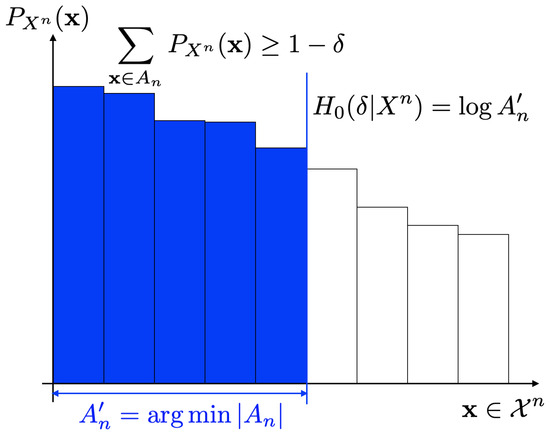
Figure 1. Smooth max entropy $H_0\left(\delta \right|X^n)$.

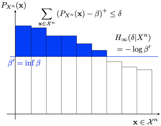
Figure 2. Smooth min entropy $H_{\infty }\left(\delta \right|X^n)$.

In this paper, we use the above alternative expressions of the smooth max entropy and the smooth min entropy instead of (19).

3. Source Resolvability Problem

We consider the problem concerning how to simulate a given discrete source $\mathbf{X}={\left\{X^n\right\}}_{n=1}^{\infty }$ by using the uniform random number $U_{M_n}$ and the mapping ${\varphi }_n$. Figure 3 is an illustrative figure of this problem (the probability distribution for $X^n$ is depicted in black, while the one for ${\varphi }_n\left(U_{M_n}\right)$ is shown in blue). Since it is hard to simulate the exact source in general, we consider the approximation problem under some measure. This problem is called the resolvability problem. One of the main objectives in the resolvability problem is to derive the smallest value of a in the form of $M_n=e^{na}$, which we call the optimum resolvability rate [1,8]. This is formulated as follows.

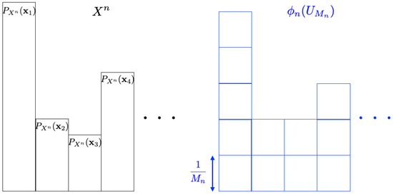
Figure 3. Resolvability problem.

Definition 3. 

Rate R is said to be D-achievable with the given f-divergence if there exists a sequence of mapping ${\varphi }_n:{\mathcal{U}}_{M_n}\to {\mathcal{X}}^n$ such that

$$\underset{n\to \infty }{lim\; sup}{D}_f(X^n\left|\right|{\varphi }_n\left(U_{M_n}\right))\le D,$$

(23)

$$\underset{n\to \infty }{lim\; sup}{\displaystyle \frac{1}{n}}log{M}_n\le R.$$

(24)

Given some D, if the rate constraint R is sufficiently large, it can be shown that there exists a sequence of mappings satisfying constraints in the above definition. Conversely, if R is too small, no sequence of mappings that satisfies constraints can be found. Therefore, in the resolvability problem, the infimum of R is of particular interest.

Definition 4 (First-order optimum resolvability rate).

$$\begin{array}{ccc}\hfill S_r^{\left(f\right)}\left(D\right|\mathbf{X})& :=& inf\left\{R\left|R is D-achievable with the given f-divergence\right.\right\}.\hfill \end{array}$$

(25)

Remark 6. 

It should be noted that we do not use $D_f({\varphi }_n\left(U_{M_n}\right)\left|\right|X^n)$ but $D_f(X^n\left|\right|{\varphi }_n\left(U_{M_n}\right))$ as a condition in Definition 3. This is important to consider the asymmetric measure such as the KL-divergence.

Remark 7. 

We consider the case where D is in $[0,f(0\left)\right)$ under the given f-divergence. Since $f\left(t\right)$ is defined in the range $t>0$ and we assume that the function $f\left(t\right)$ is a decreasing function of t, $D_f(X^n\left|\right|Y^n)\le f\left(0\right)$ holds for any distributions $P_{X^n}(·)$ and $P_{Y^n}(·)$ from the definition of f-divergence. Hence, $D\ge f\left(0\right)$ means that there exists no restriction about the approximation error (for example, $f\left(0\right)=1$ in the case of the half variational distance and $f\left(0\right)=\infty$ in the case of the KL divergence). This case leads to the trivial result that the first-order optimum resolvability rate equals 0. Hence, we only consider the case of $D\in [0,f(0\left)\right)$. A similar observation is applicable throughout the following sections.

Our main objective in this section is to derive the general formula of the first-order optimum resolvability rate. To do so, we first derive the following two theorems. We use the notation $f^{-1}\left(a\right)=inf\left\{t\right|f\left(t\right)=a\}.$

Theorem 3. 

Under conditions C1)–C3), for any $\gamma >0$ and any $M_n$ satisfying

$${\displaystyle \frac{1}{n}}log{M}_n\ge {\displaystyle \frac{1}{n}}{H}_0(1-f^{-1}\left(D\right)|X^n)+\gamma ,$$

(26)

there exists a mapping ${\varphi }_n$, which satisfies

$$D_f(X^n\left|\right|{\varphi }_n\left(U_{M_n}\right))\le D+\gamma$$

(27)

for sufficiently large n.

Proof. 

We arbitrarily fix $M_n$ satisfying (26). We show that there exists a mapping ${\varphi }_n$ that satisfies (27) for sufficiently large n. Let $B_n\subset {\mathcal{X}}^n$ denote a set satisfying

$$Pr\{X^n\in B_n\}\ge f^{-1}\left(D\right)$$

(28)

and

$$log|B_n|=H_0(1-f^{-1}\left(D\right)|X^n).$$

(29)

The existence of the above set $B_n$ is guaranteed by (21). We define the probability distribution $P_{{\overline{X}}^n}$ over $B_n$ as

$$P_{{\overline{X}}^n}\left(\mathbf{x}\right):=\left\{\begin{array}{cc}{\displaystyle \frac{P_{X^n}\left(\mathbf{x}\right)}{Pr\{X^n\in B_n\}}}& \mathbf{x}\in B_n,\\ 0& otherwise.\end{array}\right.$$

(30)

Furthermore, let a set $C_n$ be as

$$C_n:=\left\{\mathbf{x}\in B_n\left|P_{{\overline{X}}^n}\left(\mathbf{x}\right)\ge {\displaystyle \frac{1}{M_n}}\right.\right\}$$

(31)

and arrange elements in $C_n$ as

$$C_n=\{{\mathbf{x}}_1,{\mathbf{x}}_2,\cdots ,{\mathbf{x}}_{|C_n|}\}$$

(32)

according to $P_{{\overline{X}}^n}\left(\mathbf{x}\right)$ in ascendant order. That is, $P_{{\overline{X}}^n}\left({\mathbf{x}}_i\right)\le P_{{\overline{X}}^n}\left({\mathbf{x}}_j\right)(1\le i<j\le |C_n\left|\right)$ holds. Here, we define $i^{\ast }:=\left|C_n\right|$ and index $\mathbf{x}\in B_n\setminus C_n$ as ${\mathbf{x}}_{i^{\ast }+1},{\mathbf{x}}_{i^{\ast }+2},\cdots ,{\mathbf{x}}_{|B_n|}$ arbitrarily.

Then, from the above definition, it holds that

$$P_{{\overline{X}}^n}\left({\mathbf{x}}_{i^{\ast }}\right)=\underset{\mathbf{x}\in C_n}{max}{P}_{{\overline{X}}^n}\left(\mathbf{x}\right).$$

(33)

Thus, from the assumption (15), for any small $\epsilon \in (0,\underline{H}\left(\mathbf{X}\right))$, it holds that

$$P_{{\overline{X}}^n}\left({\mathbf{x}}_{i^{\ast }}\right)\ge e^{-n(\underline{H}\left(\mathbf{X}\right)-\epsilon )}$$

(34)

for sufficiently large n.

Set $k_0=0$. For ${\mathbf{x}}_1$ we determine $k_1$ such that

$${\displaystyle \frac{k_1}{M_n}}\le P_{{\overline{X}}^n}\left({\mathbf{x}}_1\right),{\displaystyle \frac{k_1+1}{M_n}}>P_{{\overline{X}}^n}\left({\mathbf{x}}_1\right).$$

(35)

Secondly, we determine $k_2$ for ${\mathbf{x}}_2$ such that

$${\displaystyle \frac{k_2-k_1}{M_n}}\le P_{{\overline{X}}^n}\left({\mathbf{x}}_2\right),{\displaystyle \frac{k_2-k_1+1}{M_n}}>P_{{\overline{X}}^n}\left({\mathbf{x}}_2\right).$$

(36)

In a similar way, we repeat this operation to choose $k_i$ for ${\mathbf{x}}_i$ as long as possible. Then, it is not difficult to check that the above procedure does not stop before $i<i^{\ast }$.

We define a mapping ${\varphi }_n:{\mathcal{U}}_{M_n}\to {\mathcal{X}}^n$ as

$${\varphi }_n\left(j\right)=\left\{\begin{array}{cc}{\mathbf{x}}_i\hfill & k_{i-1}+1\le j\le k_i,i<i^{\ast }\hfill \\ {\mathbf{x}}_{i^{\ast }}\hfill & \mathrm{otherwise}\hfill \end{array}\right.$$

(37)

and set ${\tilde{X}}^n={\varphi }_n\left(U_{M_n}\right)$.

We evaluate the performance of the mapping ${\varphi }_n$. From the construction of the mapping, for any i satisfying $1\le i\le i^{\ast }-1$ it holds that

$$P_{{\tilde{X}}^n}\left({\mathbf{x}}_i\right)\le P_{{\overline{X}}^n}\left({\mathbf{x}}_i\right)$$

(38)

$$P_{{\overline{X}}^n}\left({\mathbf{x}}_i\right)<P_{{\tilde{X}}^n}\left({\mathbf{x}}_i\right)+{\displaystyle \frac{1}{M_n}}.$$

(39)

We next evaluate $P_{{\tilde{X}}^n}\left({\mathbf{x}}_{i^{\ast }}\right)$. From the construction, we have $P_{{\overline{X}}^n}\left({\mathbf{x}}_{i^{\ast }}\right)\le P_{{\tilde{X}}^n}\left({\mathbf{x}}_{i^{\ast }}\right)$. Since $P_{{\tilde{X}}^n}\left({\mathbf{x}}_i\right)=0$ holds for $\forall i\in B_n\setminus C_n$, we obtain

$$P_{{\overline{X}}^n}\left({\mathbf{x}}_i\right)-P_{{\tilde{X}}^n}\left({\mathbf{x}}_i\right)=P_{{\overline{X}}^n}\left({\mathbf{x}}_i\right)<{\displaystyle \frac{1}{M_n}}$$

(40)

for $\forall i\in B_n\setminus C_n$. Hence, also from the construction of the mapping, we obtain

$$\begin{array}{ccc}\hfill P_{{\tilde{X}}^n}\left({\mathbf{x}}_{i^{\ast }}\right)-P_{{\overline{X}}^n}\left({\mathbf{x}}_{i^{\ast }}\right)& =& \left(1-\sum _{i=1}^{i^{\ast }-1}{P}_{{\tilde{X}}^n}\left({\mathbf{x}}_i\right)\right)-\left(1-\sum _{{\mathbf{x}}_i\in B_n\setminus \left\{{\mathbf{x}}_{i^{\ast }}\right\}}{P}_{{\overline{X}}^n}\left({\mathbf{x}}_i\right)\right)\hfill \\ & =& \sum _{{\mathbf{x}}_i\in B_n\setminus \left\{{\mathbf{x}}_{i^{\ast }}\right\}}{P}_{{\overline{X}}^n}\left({\mathbf{x}}_i\right)-\sum _{{\mathbf{x}}_i\in B_n\setminus \left\{{\mathbf{x}}_{i^{\ast }}\right\}}{P}_{{\tilde{X}}^n}\left({\mathbf{x}}_i\right)\hfill \\ & =& \sum _{{\mathbf{x}}_i\in B_n\setminus \left\{{\mathbf{x}}_{i^{\ast }}\right\}}\left(P_{{\overline{X}}^n}\left({\mathbf{x}}_i\right)-P_{{\tilde{X}}^n}\left({\mathbf{x}}_i\right)\right)\hfill \\ & \le & {\displaystyle \frac{|B_n|}{M_n}}\hfill \\ & \le & e^{-n\gamma },\hfill \end{array}$$

(41)

where the second equality is from the fact that $P_{{\tilde{X}}^n}\left({\mathbf{x}}_i\right)=0$ for $\forall i\in B_n\setminus C_n$, the first inequality is due to (39) and (40), and the last inequality is obtained from (26) and (29). Thus, we have

$$P_{{\tilde{X}}^n}\left({\mathbf{x}}_{i^{\ast }}\right)\le P_{{\overline{X}}^n}\left({\mathbf{x}}_{i^{\ast }}\right)+e^{-n\gamma }.$$

(42)

From the above argument, the f-divergence is given by

$$\begin{array}{ccc}\hfill D_f\left(X^n\left|\right|{\varphi }_n\left(U_{M_n}\right)\right)& =& \sum _{i=1}^{i^{\ast }}{P}_{{\tilde{X}}^n}\left({\mathbf{x}}_i\right)f\left({\displaystyle \frac{P_{X^n}\left({\mathbf{x}}_i\right)}{P_{{\tilde{X}}^n}\left({\mathbf{x}}_i\right)}}\right)\hfill \\ & =& \sum _{i=1}^{i^{\ast }}{P}_{{\tilde{X}}^n}\left({\mathbf{x}}_i\right)f\left({\displaystyle \frac{P_{{\overline{X}}^n}\left({\mathbf{x}}_i\right)Pr\left\{X^n\in B_n\right\}}{P_{{\tilde{X}}^n}\left({\mathbf{x}}_i\right)}}\right)\hfill \\ & =& \sum _{i=1}^{i^{\ast }-1}{P}_{{\tilde{X}}^n}\left({\mathbf{x}}_i\right)f\left({\displaystyle \frac{P_{{\overline{X}}^n}\left({\mathbf{x}}_i\right)Pr\left\{X^n\in B_n\right\}}{P_{{\tilde{X}}^n}\left({\mathbf{x}}_i\right)}}\right)\hfill \\ & & +P_{{\tilde{X}}^n}\left({\mathbf{x}}_{i^{\ast }}\right)f\left({\displaystyle \frac{P_{{\overline{X}}^n}\left({\mathbf{x}}_{i^{\ast }}\right)Pr\left\{X^n\in B_n\right\}}{P_{{\tilde{X}}^n}\left({\mathbf{x}}_{i^{\ast }}\right)}}\right)\hfill \\ & \le & \sum _{i=1}^{i^{\ast }-1}{P}_{{\tilde{X}}^n}\left({\mathbf{x}}_i\right)f\left(Pr\left\{X^n\in B_n\right\}\right)\hfill \\ & & +P_{{\tilde{X}}^n}\left({\mathbf{x}}_{i^{\ast }}\right)f\left({\displaystyle \frac{P_{{\overline{X}}^n}\left({\mathbf{x}}_{i^{\ast }}\right)Pr\left\{X^n\in B_n\right\}}{P_{{\tilde{X}}^n}\left({\mathbf{x}}_{i^{\ast }}\right)}}\right),\hfill \end{array}$$

(43)

where the first equality is due to the condition C2) and the last inequality is due to (38) and the condition C1).

The second term of the RHS of (43) is evaluated as follows. From (42) and C1), we have

$$\begin{array}{c}{\displaystyle P_{{\tilde{X}}^n}\left({\mathbf{x}}_{i^{\ast }}\right)f\left(\frac{P_{{\overline{X}}^n}\left({\mathbf{x}}_{i^{\ast }}\right)Pr\left\{X^n\in B_n\right\}}{P_{{\tilde{X}}^n}\left({\mathbf{x}}_{i^{\ast }}\right)}\right)}\hfill \\ \hspace{1em}\le \left(P_{{\overline{X}}^n}\left({\mathbf{x}}_{i^{\ast }}\right)+e^{-n\gamma }\right)f\left({\displaystyle \frac{P_{{\overline{X}}^n}\left({\mathbf{x}}_{i^{\ast }}\right)Pr\left\{X^n\in B_n\right\}}{P_{{\overline{X}}^n}\left({\mathbf{x}}_{i^{\ast }}\right)+e^{-n\gamma }}}\right).\hfill \end{array}$$

(44)

Here, using the relation

$$\begin{array}{c}{\displaystyle P_{{\overline{X}}^n}\left({\mathbf{x}}_{i^{\ast }}\right)Pr\left\{X^n\in B_n\right\}}\hfill \\ \hspace{1em}=(1-e^{-n\gamma })P_{{\overline{X}}^n}\left({\mathbf{x}}_{i^{\ast }}\right)Pr\left\{X^n\in B_n\right\}+e^{-n\gamma }{P}_{{\overline{X}}^n}\left({\mathbf{x}}_{i^{\ast }}\right)Pr\left\{X^n\in B_n\right\},\hfill \end{array}$$

(45)

we obtain

$$\begin{array}{c}{\displaystyle \left(P_{{\overline{X}}^n}\left({\mathbf{x}}_{i^{\ast }}\right)+e^{-n\gamma }\right)f\left(\frac{P_{{\overline{X}}^n}\left({\mathbf{x}}_{i^{\ast }}\right)Pr\left\{X^n\in B_n\right\}}{P_{{\overline{X}}^n}\left({\mathbf{x}}_{i^{\ast }}\right)+e^{-n\gamma }}\right)}\hfill \\ \hspace{1em}\le P_{{\overline{X}}^n}\left({\mathbf{x}}_{i^{\ast }}\right)f\left({\displaystyle \frac{(1-e^{-n\gamma })P_{{\overline{X}}^n}\left({\mathbf{x}}_{i^{\ast }}\right)Pr\left\{X^n\in B_n\right\}}{P_{{\overline{X}}^n}\left({\mathbf{x}}_{i^{\ast }}\right)}}\right)\hfill \\ \hspace{1em}\hspace{1em}+e^{-n\gamma }f\left({\displaystyle \frac{e^{-n\gamma }{P}_{{\overline{X}}^n}\left({\mathbf{x}}_{i^{\ast }}\right)Pr\left\{X^n\in B_n\right\}}{e^{-n\gamma }}}\right)\hfill \\ \hspace{1em}=P_{{\overline{X}}^n}\left({\mathbf{x}}_{i^{\ast }}\right)f\left((1-e^{-n\gamma })Pr\left\{X^n\in B_n\right\}\right)\hfill \\ \hspace{1em}\hspace{1em}+e^{-n\gamma }f\left(P_{{\overline{X}}^n}\left({\mathbf{x}}_{i^{\ast }}\right)Pr\left\{X^n\in B_n\right\}\right)\hfill \\ \hspace{1em}\le P_{{\overline{X}}^n}\left({\mathbf{x}}_{i^{\ast }}\right)f\left((1-e^{-n\gamma })Pr\left\{X^n\in B_n\right\}\right)\hfill \\ \hspace{1em}\hspace{1em}+e^{-n\gamma }f\left(e^{-n(\underline{H}\left(\mathbf{X}\right)-\epsilon )}Pr\left\{X^n\in B_n\right\}\right)\hfill \end{array}$$

(46)

for sufficiently large n, where the first inequality is due to (11) and the last inequality is from (34) and the condition C1).

Hence, from C3) and the continuity of the function f, for $\forall \nu >0$ we have

$$\begin{array}{c}{\displaystyle \left(P_{{\overline{X}}^n}\left({\mathbf{x}}_{i^{\ast }}\right)+e^{-n\gamma }\right)f\left(\frac{P_{{\overline{X}}^n}\left({\mathbf{x}}_{i^{\ast }}\right)Pr\left\{X^n\in B_n\right\}}{P_{{\overline{X}}^n}\left({\mathbf{x}}_{i^{\ast }}\right)+e^{-n\gamma }}\right)}\hfill \\ \hspace{1em}\le P_{{\overline{X}}^n}\left({\mathbf{x}}_{i^{\ast }}\right)f\left(Pr\left\{X^n\in B_n\right\}-e^{-n\gamma }\right)+\nu \hfill \\ \hspace{1em}\le P_{{\overline{X}}^n}\left({\mathbf{x}}_{i^{\ast }}\right)f\left(Pr\left\{X^n\in B_n\right\}\right)+2\nu \hfill \end{array}$$

(47)

for sufficiently large n. Therefore, noting that $P_{{\overline{X}}^n}\left({\mathbf{x}}_{i^{\ast }}\right)\le P_{{\tilde{X}}^n}\left({\mathbf{x}}_{i^{\ast }}\right)$, from (28), (43), (44) and (47) it holds that

$$\begin{array}{ccc}\hfill D_f\left(X^n\left|\right|{\varphi }_n\left(U_{M_n}\right)\right)& \le & \sum _{i=1}^{i^{\ast }}{P}_{{\tilde{X}}^n}\left({\mathbf{x}}_i\right)f\left(Pr\left\{X^n\in B_n\right\}\right)+2\nu \hfill \\ & =& f\left(Pr\left\{X^n\in B_n\right\}\right)+2\nu \hfill \\ & \le & f\left(f^{-1}\left(D\right)\right)+2\nu \hfill \\ & =& D+2\nu \hfill \end{array}$$

(48)

for sufficiently large n. This completes the proof of the theorem. □

Theorem 4. 

Under conditions C1) and C2), for any mapping ${\varphi }_n$ satisfying

$$D_f(X^n\left|\right|{\varphi }_n\left(U_{M_n}\right))\le D,$$

(49)

it holds that

$${\displaystyle \frac{1}{n}}log{M}_n\ge {\displaystyle \frac{1}{n}}{H}_0(1-f^{-1}\left(D\right)|X^n).$$

(50)

Proof. 

It suffices to show the fact that the relation

$${\displaystyle \frac{1}{n}}log{M}_n<{\displaystyle \frac{1}{n}}{H}_0(1-f^{-1}\left(D\right)|X^n)$$

(51)

necessarily yields

$$D_f(X^n\left|\right|{\varphi }_n\left(U_{M_n}\right))>D.$$

(52)

We here denote $H^{\prime }:=H_0(1-f^{-1}\left(D\right)|X^n)$ for short. For any fixed mapping ${\varphi }_n:{\mathcal{U}}_{M_n}\to {\mathcal{X}}^n$, we set ${\tilde{X}}^n:={\varphi }_n\left(U_{M_n}\right)$ and

$$B_n:=\left\{\mathbf{x}\in {\mathcal{X}}^n|P_{{\tilde{X}}^n}\left(\mathbf{x}\right)>0\right\}.$$

(53)

Then, from the property of the mapping it must hold that

$$M_n\ge \left|B_n\right|.$$

(54)

From the condition C2) the f-divergence between $P_{X^n}$ and $P_{{\tilde{X}}^n}$ is lower bounded by

$$\begin{array}{ccc}\hfill D_f(X^n\left|\right|{\varphi }_n\left(U_{M_n}\right))& =& \sum _{\mathbf{x}\in B_n}{P}_{{\tilde{X}}^n}\left(\mathbf{x}\right)f\left({\displaystyle \frac{P_{X^n}\left(\mathbf{x}\right)}{P_{{\tilde{X}}^n}\left(\mathbf{x}\right)}}\right)\hfill \\ & \ge & f\left(Pr\{X^n\in B_n\}\right)\hfill \\ & \ge & f\left(\underset{\begin{array}{c}{B}_n\subset {\mathcal{X}}^n\\ |B_n|\le M_n\end{array}}{max}Pr\{X^n\in B_n\}\right)\hfill \\ & \ge & f\left(\underset{\begin{array}{c}{B}_n\subset {\mathcal{X}}^n\\ log|B_n|<H^{\prime }\end{array}}{max}Pr\{X^n\in B_n\}\right)\hfill \\ & >& f\left(1-(1-f^{-1}\left(D\right))\right)\hfill \\ & =& D,\hfill \end{array}$$

(55)

where the first inequality is due to (11), the second inequality is due to condition C1) and (54) and the third inequality is from (51). The last inequality is from the definition of the alternative expressions given in Theorem 1. This completes the proof. □

Theorems 3 and 4 show that the smooth max entropy and the inverse function of f have important roles in the resolvability problem with respect to f-divergences. From these theorems, we obtain the following theorem, which addresses the general formula of the optimum resolvability rate. It should be noted that because of the assumption $0\le D<f\left(0\right)$ and C1), we have $0<f^{-1}\left(D\right)\le 1$.

Theorem 5. 

Under conditions C1)–C3), it holds that

$$\begin{array}{cc}\hfill S_r^{\left(f\right)}\left(D\right|\mathbf{X})& =\underset{\nu \downarrow 0}{lim}\underset{n\to \infty }{lim\; sup}{\displaystyle \frac{1}{n}}{H}_0(1-f^{-1}(D+\nu )|X^n)\hfill \\ \hfill & =\underset{\nu \downarrow 0}{lim}\underset{n\to \infty }{lim\; sup}{\displaystyle \frac{1}{n}}{H}_0(1-f^{-1}\left(D\right)+\nu |X^n).\hfill \end{array}$$

(56)

Proof. 

We here show the first equality, because the second equality can be derived from the first inequality together with the continuity of the function $f^{-1}$.

(Direct Part:) Fix $\nu >0$ arbitrarily. From Theorem 3, for any $\gamma >0$, there exists a mapping ${\varphi }_n$ such that

$$\begin{array}{ccc}\hfill {\displaystyle \frac{1}{n}}log{M}_n& \le & {\displaystyle \frac{1}{n}}{H}_0(1-f^{-1}(D+\nu )|X^n)+\gamma ,\hfill \end{array}$$

(57)

and

$$D_f(X^n\left|\right|{\varphi }_n\left(U_{M_n}\right))\le D+\nu +\gamma .$$

(58)

We here use the diagonal line argument [8]. Fix a sequence ${\left\{{\gamma }_i\right\}}_{i=1}^{\infty }$ such that ${\gamma }_1>{\gamma }_2>\cdots >0$, and we repeat the above argument as $i\to \infty$. Then, we can show that there exists a mapping ${\varphi }_n$ satisfying

$$\underset{n\to \infty }{lim\; sup}{D}_f(X^n\left|\right|{\varphi }_n\left(U_{M_n}\right))\le D+\nu ,$$

(59)

and

$$\begin{array}{c}\hfill \underset{n\to \infty }{lim\; sup}{\displaystyle \frac{1}{n}}log{M}_n\le \underset{n\to \infty }{lim\; sup}{\displaystyle \frac{1}{n}}{H}_0(1-f^{-1}(D+\nu )|X^n).\end{array}$$

(60)

Here, also from the diagonal line argument with respect to $\nu$, we obtain

$$\begin{array}{c}\hfill \underset{n\to \infty }{lim\; sup}{\displaystyle \frac{1}{n}}log{M}_n\le \underset{\nu \downarrow 0}{lim}\underset{n\to \infty }{lim\; sup}{\displaystyle \frac{1}{n}}{H}_0(1-f^{-1}(D+\nu )|X^n).\end{array}$$

(61)

This completes the proof of the direct part.

(Converse Part:) We fixed $\nu >0$ arbitrarily. From Theorem 4, for any mapping ${\varphi }_n$ satisfying

$$D_f(X^n\left|\right|{\varphi }_n\left(U_{M_n}\right))\le D+\nu ,$$

(62)

it holds that

$${\displaystyle \frac{1}{n}}log{M}_n\ge {\displaystyle \frac{1}{n}}{H}_0(1-f^{-1}(D+\nu )|X^n).$$

(63)

Consequently, we have

$$\underset{n\to \infty }{lim\; sup}{D}_f(X^n\left|\right|{\varphi }_n\left(U_{M_n}\right))\le D+\nu$$

(64)

and

$$\underset{n\to \infty }{lim\; sup}{\displaystyle \frac{1}{n}}log{M}_n\ge \underset{n\to \infty }{lim\; sup}{\displaystyle \frac{1}{n}}{H}_0(1-f^{-1}(D+\nu )|X^n).$$

(65)

We also use the diagonal line argument [8]. We repeat the above argument as $i\to \infty$ for a sequence ${\left\{{\nu }_i\right\}}_{i=1}^{\infty }$ such that ${\nu }_1>{\nu }_2>\cdots >0$. Then, for any mapping ${\varphi }_n$ satisfying

$$\underset{n\to \infty }{lim\; sup}{D}_f(X^n\left|\right|{\varphi }_n\left(U_{M_n}\right))\le D,$$

(66)

it holds that

$$\begin{array}{ccc}\hfill \underset{n\to \infty }{lim\; sup}{\displaystyle \frac{1}{n}}log{M}_n& \ge & \underset{\nu \downarrow 0}{lim}\underset{n\to \infty }{lim\; sup}{\displaystyle \frac{1}{n}}{H}_0(1-f^{-1}(D+\nu )|X^n).\hfill \end{array}$$

(67)

This completes the proof of the converse part. □

4. Intrinsic Randomness Problem

In the previous section, we reveal the general formula for the optimum resolvability rate. In this section, we consider how to approximate the uniform random number $U_{M_n}$ by using the given discrete source $\mathbf{X}={\left\{X^n\right\}}_{n=1}^{\infty }$ and the mapping ${\phi }_n$. Figure 4 is an illustrative figure of the problem (the probability distribution for $U_{M_n}$ is depicted in blue, while the one for ${\phi }_n\left(X^n\right)$ is shown in black). The size of the random number $M_n$ is requested to be as large as possible. In the intrinsic randomness problem, one of our main concerns is to derive the largest value of b in the form of $M_n=e^{nb}$ under some approximation measure [7]. This problem setting is formulated as follows.

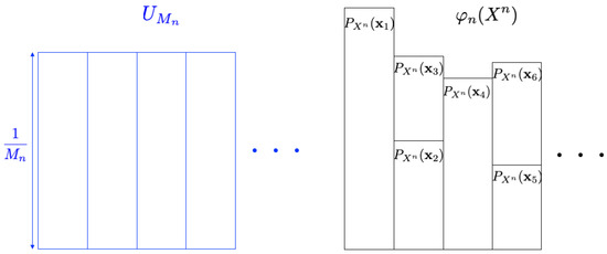
Figure 4. Intrinsic randomness problem.

Definition 5. 

R is said to be Δ-achievable with the given f-divergence if there exists a sequence of mapping ${\phi }_n:{\mathcal{X}}^n\to {\mathcal{U}}_{M_n}$ such that

$$\begin{array}{ccc}\hfill \underset{n\to \infty }{lim\; sup}{D}_f({\phi }_n\left(X^n\right)\left|\right|U_{M_n})& \le & \Delta ,\hfill \end{array}$$

(68)

$$\begin{array}{ccc}\hfill \underset{n\to \infty }{lim\; inf}{\displaystyle \frac{1}{n}}log{M}_n& \ge & R.\hfill \end{array}$$

(69)

In this case, given $\Delta$, if the rate constraint R is sufficiently small, it can be shown that there exists a sequence of mappings that satisfies the constraints. On the other hand, if R is too large, no sequence of mappings that achieves the desired constraints can be found. Consequently, in this setting, the supremum of R is of particular interest.

Definition 6 (First-order optimum intrinsic randomness rate).

$$S_{\iota }^{\left(f\right)}(\Delta |\mathbf{X}):=sup\left\{R\left|R is \Delta -achievable with the given f-divergence\right.\right\}.$$

(70)

Remark 8. 

It should be emphasized that we use the f-divergence of the form $D_f({\phi }_n\left(X^n\right)\left|\right|U_{M_n})$ instead of $D_f(U_{M_n}\left|\right|{\phi }_n\left(X^n\right))$ (cf. Remark 6).

We also assume that $\Delta \in [0,f(0\left)\right)$ in this section (cf. Remark 7). In order to analyze the general formula of the optimum intrinsic randomness rate $S_{\iota }^{\left(f\right)}(\Delta |\mathbf{X})$, we first give two theorems.

Theorem 6. 

Under conditions C1) and C2), for any $\gamma >0$ and $M_n$ satisfying

$${\displaystyle \frac{1}{n}}log{M}_n\le {\displaystyle \frac{1}{n}}{H}_{\infty }(1-f^{-1}(\Delta )|X^n)-\gamma ,$$

(71)

there exists a mapping ${\phi }_n$ such that

$$D_f({\phi }_n\left(X^n\right)\left|\right|U_{M_n})\le \Delta +\gamma$$

(72)

for sufficiently large n.

Proof. 

We set ${\beta }_0$ as

$$-log{\beta }_0=H_{\infty }(1-f^{-1}(\Delta )|X^n)$$

(73)

for short.

From Theorem 2, we notice that

$$1-f^{-1}(\Delta )\ge \sum _{\mathbf{x}\in {\mathcal{X}}^n}{\left(P_{X^n}\left(\mathbf{x}\right)-{\beta }_0\right)}^{+}=:1-A_n(\Delta ),$$

(74)

where if ${\beta }_0>1/\left|{\mathcal{X}}^n\right|$ holds, then $f^{-1}(\Delta )=A_n(\Delta )$. We shall show that for any $M_n$ satisfying

$${\displaystyle \frac{1}{n}}log{M}_n\le -{\displaystyle \frac{1}{n}}log{\beta }_0-{\displaystyle \frac{1}{n}}log{\displaystyle \frac{1}{A_n(\Delta )}}-{\displaystyle \frac{\gamma }{2}},$$

(75)

there exists a mapping ${\phi }_n$ such that

$$D_f({\phi }_n\left(X^n\right)\left|\right|U_{M_n})\le \Delta +\gamma$$

(76)

for sufficiently large n.

For every sequence $\mathbf{x}\in {\mathcal{X}}^n$, we define the probability distribution

$$P_{{\overline{X}}^n}\left(\mathbf{x}\right):=\left\{\begin{array}{cc}{\displaystyle \frac{{\beta }_0}{A_n(\Delta )}}& P_{X^n}\left(\mathbf{x}\right)\ge {\beta }_0,\\ {\displaystyle \frac{P_{X^n}\left(\mathbf{x}\right)}{A_n(\Delta )}}& P_{X^n}\left(\mathbf{x}\right)<{\beta }_0.\end{array}\right.$$

(77)

Since $0<A_n(\Delta )<1$, this probability distribution is well-defined. Then, from the definition of the smooth min entropy it holds that

$$\sum _{\mathbf{x}\in {\mathcal{X}}^n}{P}_{{\overline{X}}^n}\left(\mathbf{x}\right)=1.$$

(78)

Here, from (75) and the definition of the smooth min entropy it holds that

$$\begin{array}{cc}\hfill M_n& \le {\displaystyle \frac{1}{{\beta }_0}}{A}_n(\Delta )e^{-n\gamma /2}\le \left|{\mathcal{X}}^n\right|\hfill \end{array}$$

(79)

for sufficiently large n.

We next define the mapping ${\phi }_n:{\mathcal{X}}^n\to {\mathcal{U}}_{M_n}$ by using $P_{{\overline{X}}^n}$. To do so, we classify the elements of ${\mathcal{X}}^n$ into $I_n\left(i\right)(1\le i\le M_n)$ as follows.

• We choose a set $I_n\left(1\right)$ arbitrarily satisfying

  $$\sum _{\mathbf{x}\in I_n\left(1\right)}{P}_{{\overline{X}}^n}\left(\mathbf{x}\right)\le {\displaystyle \frac{1}{M_n}},$$

  (80)

  $$\sum _{\mathbf{x}\in I_n\left(1\right)}{P}_{{\overline{X}}^n}\left(\mathbf{x}\right)+P_{{\overline{X}}^n}\left({\mathbf{x}}^{\prime }\right)>{\displaystyle \frac{1}{M_n}}$$

  (81)

  for any ${\mathbf{x}}^{\prime }\in {\mathcal{X}}^n\setminus I_n\left(1\right)$.
• Next, we choose a set $I_n\left(2\right)\subset {\mathcal{X}}^n\setminus I_n\left(1\right)$ satisfying

  $$\sum _{\mathbf{x}\in I_n\left(2\right)}{P}_{{\overline{X}}^n}\left(\mathbf{x}\right)\le {\displaystyle \frac{1}{M_n}},$$

  (82)

  $$\sum _{\mathbf{x}\in I_n\left(2\right)}{P}_{{\overline{X}}^n}\left(\mathbf{x}\right)+P_{{\overline{X}}^n}\left({\mathbf{x}}^{\prime }\right)>{\displaystyle \frac{1}{M_n}}$$

  (83)

  for any ${\mathbf{x}}^{\prime }\in {\mathcal{X}}^n\setminus {\bigcup }_{i=1}^2{I}_n\left(i\right)$.

Furthermore, we repeat this operation $(M_n-1)$ times so as to choose sets $I_n\left(i\right)(1\le i\le M_n-1)$. Notice here that since ${\displaystyle \frac{1}{M_n}}>{\displaystyle \frac{{\beta }_0}{A_n(\Delta )}}$ holds, we can repeat this operation $(M_n-1)$ times. Thus, from the above procedure, all of $I_n\left(i\right)(1\le i\le M_n-1)$ are not empty. Lastly, we set $I_n\left(M_n\right)=\{\mathbf{x}\in {\mathcal{X}}^n|\mathbf{x}\in {\mathcal{X}}^n\setminus {\cup }_{i=1}^{M_n-1}{I}_n\left(i\right))\}$.

From $I_n\left(i\right)(1\le i\le M_n)$, we define the mapping ${\phi }_n:{\mathcal{X}}^n\to {\mathcal{U}}_{M_n}$ as follows:

$${\phi }_n\left(\mathbf{x}\right)=i,\mathbf{x}\in I_n\left(i\right).$$

(84)

Furthermore, we set ${\tilde{U}}_{M_n}={\phi }_n\left(X^n\right)$. Thus,

$$P_{{\tilde{U}}_{M_n}}\left(i\right)=\sum _{\mathbf{x}\in I_n\left(i\right)}{P}_{X^n}\left(\mathbf{x}\right)$$

(85)

holds for every i in $1\le i\le M_n$.

We next evaluate the above mapping ${\phi }_n$. From the construction of the mapping, it holds that

$${\displaystyle \frac{1}{M_n}}<\sum _{\mathbf{x}\in I_n\left(i\right)}{P}_{{\overline{X}}^n}\left(\mathbf{x}\right)+{\displaystyle \frac{{\beta }_0}{A_n(\Delta )}}$$

(86)

for all $i(1\le i\le M_n-1)$ and

$${\displaystyle \frac{1}{M_n}}\le \sum _{\mathbf{x}\in I_n\left(M_n\right)}{P}_{{\overline{X}}^n}\left(\mathbf{x}\right).$$

(87)

Hence, for all $i(1\le i\le M_n)$, we have

$${\displaystyle \frac{1}{M_n}}-{\displaystyle \frac{{\beta }_0}{A_n(\Delta )}}\le \sum _{\mathbf{x}\in I_n\left(i\right)}{P}_{{\overline{X}}^n}\left(\mathbf{x}\right).$$

(88)

Here, notice that for all $\mathbf{x}\in {\mathcal{X}}^n$

$$P_{{\overline{X}}^n}\left(\mathbf{x}\right)\le {\displaystyle \frac{P_{X^n}\left(\mathbf{x}\right)}{A_n(\Delta )}}$$

(89)

holds from (77). Thus, we have

$$\begin{array}{ccc}\hfill {\displaystyle \frac{P_{{\tilde{U}}_{M_n}}\left(i\right)}{A_n(\Delta )}}& =& {\displaystyle \frac{{\sum }_{\mathbf{x}\in I_n\left(i\right)}{P}_{X^n}\left(\mathbf{x}\right)}{A_n(\Delta )}}\hfill \\ & \ge & \sum _{\mathbf{x}\in I_n\left(i\right)}{P}_{{\overline{X}}^n}\left(\mathbf{x}\right)\hfill \\ & >& {\displaystyle \frac{1}{M_n}}-{\displaystyle \frac{{\beta }_0}{A_n(\Delta )}}\hfill \\ & =& {\displaystyle \frac{1}{M_n}}\left(1-{\displaystyle \frac{M_n{\beta }_0}{A_n(\Delta )}}\right)\hfill \\ & \ge & {\displaystyle \frac{1}{M_n}}\left(1-e^{-n\gamma /2}\right)\hfill \end{array}$$

(90)

for all $i(1\le i\le M_n)$ where the first equality is due to (85), the first inequality is due to (89), the second inequality is due to (88), and the last inequality is due to (79). Hence, we obtain

$$\begin{array}{ccc}\hfill D_f({\phi }_n\left(X^n\right)\left|\right|U_{M_n})& =& \sum _{1\le i\le M_n}{\displaystyle \frac{1}{M_n}}f\left({\displaystyle \frac{P_{{\tilde{U}}_{M_n}}\left(i\right)}{\frac{1}{M_n}}}\right)\hfill \\ & \le & \sum _{1\le i\le M_n}{\displaystyle \frac{1}{M_n}}f\left(A_n(\Delta )(1-e^{-n\gamma /2})\right)\hfill \\ & \le & f\left(f^{-1}(\Delta )\right)+{\delta }_n\hfill \\ & =& \Delta +{\delta }_n,\hfill \end{array}$$

(91)

where we can choose some ${\delta }_n>0$ such that ${\delta }_n\to 0(n\to \infty )$, the first inequality is due to (90), and the second inequality is due to the continuity of the function f, (74) and C1). This completes the proof of the theorem. □

Theorem 7. 

Under conditions C1) and C2), for any $\epsilon >0$ if the mapping ${\phi }_n$ satisfies

$$D_f({\phi }_n\left(X^n\right)\left|\right|U_{M_n})\le \Delta -\epsilon ,$$

(92)

then it holds that

$${\displaystyle \frac{1}{n}}log{M}_n\le {\displaystyle \frac{1}{n}}{H}_{\infty }(1-f^{-1}(\Delta )|X^n)$$

(93)

for sufficiently large n.

Proof. 

Setting

$$H^{\prime }:=H_{\infty }(1-f^{-1}(\Delta )|X^n),$$

(94)

we only consider the case where $H^{\prime }<\left|{\mathcal{X}}^n\right|$ holds, because $H^{\prime }=\left|{\mathcal{X}}^n\right|$ means the trivial result. Let $\epsilon >0$ be fixed arbitrarily. We show that if

$${\displaystyle \frac{1}{n}}log{M}_n>{\displaystyle \frac{1}{n}}{H}^{\prime }$$

(95)

holds for infinitely many $n=n_1,n_2,\cdots ,$ then for any ${\phi }_n$ it holds that

$$D_f({\phi }_n\left(X^n\right)\left|\right|U_{M_n})>\Delta -\epsilon .$$

(96)

From (95), there exists a positive constant $\gamma$ satisfying

$${\displaystyle \frac{1}{n}}log{M}_n-2\gamma >{\displaystyle \frac{1}{n}}{H}^{\prime }.$$

(97)

Here, for $\gamma >0$ satisfying the above inequality we set $T_n$ as

$$\begin{array}{cc}\hfill T_n& :=\left\{\mathbf{x}\in {\mathcal{X}}^n\left|{\displaystyle \frac{1}{n}}log{\displaystyle \frac{1}{P_{X^n}\left(\mathbf{x}\right)}}\le {\displaystyle \frac{1}{n}}{H}^{\prime }+\gamma \right.\right\}\hfill \end{array}$$

(98)

$$\begin{array}{cc}\hfill & =\left\{\mathbf{x}\in {\mathcal{X}}^n\left|P_{X^n}\left(\mathbf{x}\right)\ge e^{-(H^{\prime }+n\gamma )}\right.\right\}.\hfill \end{array}$$

(99)

Then, from the relation

$$\begin{array}{c}\hfill 1\ge \sum _{\mathbf{x}\in T_n}{P}_{X^n}\left(\mathbf{x}\right)\ge \left|T_n\right|e^{-(H^{\prime }+n\gamma )}\end{array}$$

(100)

we have

$$|T_n|\le e^{H^{\prime }+n\gamma }.$$

(101)

Next, we fix $M_n$ and a mapping ${\phi }_n$ satisfying (95) and set ${\tilde{U}}_{M_n}$ as ${\tilde{U}}_{M_n}={\phi }_n\left(X^n\right)$. Using ${\phi }_n$ and $T_n$, we set $I_n$ as

$$I_n:=\left\{i\right|\exists \mathbf{x}\in T_n,{\phi }_n\left(\mathbf{x}\right)=i\}.$$

(102)

Thus, the set $I_n$ is the set of index i constructing from at least one $\mathbf{x}\in T_n$ and the set ${\left(I_n\right)}^c$ is the set of i constructing only from $\mathbf{x}\in {\left(T_n\right)}^c$.

Then, from the definition of the mapping and (101), it holds that

$$|I_n|\le |T_n|\le e^{H^{\prime }+n\gamma }.$$

(103)

On the other hand, from (97), we have

$$\begin{array}{c}\hfill M_n>e^{H^{\prime }+2n\gamma }.\end{array}$$

(104)

This means that

$${\displaystyle \frac{|I_n|}{M_n}}\le e^{-n\gamma }$$

(105)

holds. Hence, from the condition C2), we have

$${\displaystyle \frac{|I_n|}{M_n}}f\left({\displaystyle \frac{M_n}{|I_n|}}\right)\to 0(n\to \infty ).$$

(106)

From the above argument, the f-divergence between ${\phi }_n\left(X^n\right)$ and $U_{M_n}$ is evaluated as

$$\begin{array}{ccc}\hfill D_f({\phi }_n\left(X^n\right)\left|\right|U_{M_n})& =& \sum _{1\le i\le M_n}{\displaystyle \frac{1}{M_n}}f\left({\displaystyle \frac{P_{{\tilde{U}}_{M_n}}\left(i\right)}{\frac{1}{M_n}}}\right)\hfill \\ & =& \sum _{1\le i\le M_n,i\in I_n}{\displaystyle \frac{1}{M_n}}f\left({\displaystyle \frac{P_{{\tilde{U}}_{M_n}}\left(i\right)}{\frac{1}{M_n}}}\right)\hfill \\ & & +\sum _{1\le i\le M_n,i\in {\left(I_n\right)}^c}{\displaystyle \frac{1}{M_n}}f\left({\displaystyle \frac{P_{{\tilde{U}}_{M_n}}\left(i\right)}{\frac{1}{M_n}}}\right)\hfill \\ & \ge & {\displaystyle \frac{|I_n|}{M_n}}f\left({\displaystyle \frac{{\sum }_{1\le i\le M_n,i\in I_n}{P}_{{\tilde{U}}_{M_n}}\left(i\right)}{\frac{|I_n|}{M_n}}}\right)\hfill \\ & & +{\displaystyle \frac{|{\left(I_n\right)}^c|}{M_n}}f\left({\displaystyle \frac{{\sum }_{1\le i\le M_n,i\in {\left(I_n\right)}^c}{P}_{{\tilde{U}}_{M_n}}\left(i\right)}{\frac{|{\left(I_n\right)}^c|}{M_n}}}\right)\hfill \\ & \ge & {\displaystyle \frac{|I_n|}{M_n}}f\left({\displaystyle \frac{1}{\frac{|I_n|}{M_n}}}\right)+{\displaystyle \frac{|{\left(I_n\right)}^c|}{M_n}}f\left({\displaystyle \frac{{\sum }_{1\le i\le M_n,i\in {\left(I_n\right)}^c}{P}_{{\tilde{U}}_{M_n}}\left(i\right)}{\frac{|{\left(I_n\right)}^c|}{M_n}}}\right)\hfill \\ & \ge & {\displaystyle \frac{|I_n|}{M_n}}f\left({\displaystyle \frac{M_n}{|I_n|}}\right)+{\displaystyle \frac{|{\left(I_n\right)}^c|}{M_n}}f\left({\displaystyle \frac{Pr\{X^n\in {\left(T_n\right)}^c\}}{\frac{|{\left(I_n\right)}^c|}{M_n}}}\right),\hfill \end{array}$$

(107)

where the first inequality is due to (11), and the last inequality is due to the relation

$$\sum _{1\le i\le M_n,i\in {\left(I_n\right)}^c}{P}_{{\tilde{U}}_{M_n}}\left(i\right)\le Pr\{X^n\in {\left(T_n\right)}^c\}$$

(108)

and C1).

We next focus on the evaluation of the second term on the RHS of (107). From the definition of the smooth min entropy $H^{\prime }$ and Theorem 1, for any $\gamma >0$ it necessarily holds that

$$\begin{array}{c}\hfill \sum _{\mathbf{x}\in {\mathcal{X}}^n}{\left(P_{X^n}\left(\mathbf{x}\right)-e^{-(H^{\prime }+n\gamma )}\right)}^{+}\ge 1-f^{-1}(\Delta ).\end{array}$$

(109)

Thus, from the definition of $T_n$ it holds that

$$\begin{array}{ccc}\hfill \sum _{\mathbf{x}\in T_n}\left(P_{X^n}\left(\mathbf{x}\right)-e^{-(H^{\prime }+n\gamma )}\right)& =& \sum _{\mathbf{x}\in {\mathcal{X}}^n}{\left(P_{X^n}\left(\mathbf{x}\right)-e^{-(H^{\prime }+n\gamma )}\right)}^{+}\hfill \\ & \ge & 1-f^{-1}(\Delta ).\hfill \end{array}$$

(110)

Thus, we obtain

$$\begin{array}{ccc}\hfill Pr\left\{X^n\in T_n\right\}& \ge & 1-f^{-1}(\Delta ),\hfill \end{array}$$

(111)

from which it holds that

$$\begin{array}{cc}\hfill Pr\left\{X^n\in {\left(T_n\right)}^c\right\}& <1-(1-f^{-1}(\Delta ))=f^{-1}(\Delta ).\end{array}$$

(112)

Plugging the above inequality with (107), we obtain

$$\begin{array}{ccc}\hfill D_f({\phi }_n\left(X^n\right)\left|\right|U_{M_n})& >& {\displaystyle \frac{|I_n|}{M_n}}f\left({\displaystyle \frac{M_n}{|I_n|}}\right)+{\displaystyle \frac{|{\left(I_n\right)}^c|}{M_n}}f\left({\displaystyle \frac{f^{-1}(\Delta )}{\frac{|{\left(I_n\right)}^c|}{M_n}}}\right).\hfill \end{array}$$

(113)

Noticing that

$${\displaystyle \frac{|{\left(I_n\right)}^c|}{M_n}}>1-e^{-n\gamma },$$

(114)

from (105), for some ${\delta }_n\to 0$, we have

$$\begin{array}{ccc}\hfill D_f({\phi }_n\left(X^n\right)\left|\right|U_{M_n})& >& \left(1-e^{-n\gamma }\right)f\left({\displaystyle \frac{f^{-1}(\Delta )}{1-e^{-n\gamma }}}\right)-{\delta }_n\hfill \\ & =& f\left({\displaystyle \frac{f^{-1}(\Delta )}{1-e^{-n\gamma }}}\right)-e^{-n\gamma }f\left({\displaystyle \frac{f^{-1}(\Delta )}{1-e^{-n\gamma }}}\right)-{\delta }_n\hfill \\ & =& f\left(f^{-1}(\Delta )(1+{\gamma }_n^{\prime })\right)-2{\delta }_n\hfill \end{array}$$

(115)

for sufficiently large n, where we use the property (106) and the notation ${\gamma }_n^{\prime }={\displaystyle \frac{e^{-n\gamma }}{1-e^{-n\gamma }}}$. Since ${\gamma }_n^{\prime }\to 0(n\to \infty )$ holds, from the continuity of the function f, it holds that

$$\begin{array}{ccc}\hfill D_f({\phi }_n\left(X^n\right)\left|\right|U_{M_n})& >& \Delta -3{\delta }_n\hfill \\ & \ge & \Delta -\epsilon \hfill \end{array}$$

(116)

for $n=n_j,n_{j+1},\cdots ,$ with some $j\ge 1$. Therefore, we obtain the theorem. □

Theorems 6 and 7 show that the smooth min entropy and the inverse function of f have important roles in the intrinsic randomness problem with respect to f-divergences, while the smooth max entropy is important in the resolvability problem. By using the above two theorems, we obtain the following theorem. It should be noted that because of the assumption $0\le \Delta <f\left(0\right)$ and C1), we have $0<f^{-1}(\Delta )\le 1$.

Theorem 8. 

Under conditions C1) and C2), it holds that

$$\begin{array}{ccc}\hfill S_{\iota }^{\left(f\right)}(\Delta |\mathbf{X})& =& \underset{\nu \downarrow 0}{lim}\underset{n\to \infty }{lim\; inf}{\displaystyle \frac{1}{n}}{H}_{\infty }(1-f^{-1}(\Delta +\nu )|X^n)\hfill \\ & =& \underset{\nu \downarrow 0}{lim}\underset{n\to \infty }{lim\; inf}{\displaystyle \frac{1}{n}}{H}_{\infty }(1-f^{-1}(\Delta )+\nu |X^n).\hfill \end{array}$$

(117)

Proof. 

(Direct Part:) Fix $\nu >0$ arbitrarily. From Theorem 6, for any $\gamma >0$ and $M_n$ such that

$$\begin{array}{cc}\hfill {\displaystyle \frac{1}{n}}{H}_{\infty }(1-f^{-1}(\Delta +\nu )|X^n)-2\gamma & \le {\displaystyle \frac{1}{n}}log{M}_n\le {\displaystyle \frac{1}{n}}{H}_{\infty }(1-f^{-1}(\Delta )|X^n)-\gamma \hfill \end{array}$$

(118)

holds, there exists a mapping ${\phi }_n$ satisfying

$$D_f({\phi }_n\left(X^n\right)\left|\right|U_{M_n})\le \Delta +\gamma$$

(119)

for sufficiently large n.

Since $\gamma >0$ is arbitrarily, we obtain

$$\underset{n\to \infty }{lim\; inf}{\displaystyle \frac{1}{n}}log{M}_n\ge \underset{n\to \infty }{lim\; inf}{\displaystyle \frac{1}{n}}{H}_{\infty }(1-f^{-1}(\Delta +\nu )|X^n).$$

(120)

Here, we fix a sequence ${\left\{{\nu }_i\right\}}_{i=1}^{\infty }$ such that ${\nu }_1>{\nu }_2>\cdots >0$, and we repeat the above argument as $i\to \infty$. Then, we can show that there exists a mapping ${\phi }_n$ satisfying

$$\underset{n\to \infty }{lim\; inf}{\displaystyle \frac{1}{n}}log{M}_n\ge \underset{\nu \downarrow 0}{lim}\underset{n\to \infty }{lim\; inf}{\displaystyle \frac{1}{n}}{H}_{\infty }(1-f^{-1}(D+\nu )|X^n),$$

(121)

and

$$\underset{n\to \infty }{lim\; sup}{D}_f({\phi }_n\left(X^n\right)\left|\right|U_{M_n})\le \Delta .$$

(122)

This completes the proof of the direct part of the theorem.

(Converse Part:) Fix $\nu >0$ arbitrarily. From Theorem 7, for any mapping ${\phi }_n$ satisfying

$$D_f({\phi }_n\left(X^n\right)\left|\right|U_{M_n})\le \Delta +\nu ,$$

(123)

it holds that

$${\displaystyle \frac{1}{n}}log{M}_n\le {\displaystyle \frac{1}{n}}{H}_{\infty }(1-f^{-1}(\Delta +2\nu )|X^n).$$

(124)

Thus, for any $\nu >0$, we obtain

$$\underset{n\to \infty }{lim\; sup}{D}_f({\phi }_n\left(X^n\right)\left|\right|U_{M_n})\le \Delta +\nu ,$$

(125)

and

$$\underset{n\to \infty }{lim\; inf}{\displaystyle \frac{1}{n}}log{M}_n\le \underset{n\to \infty }{lim\; inf}{\displaystyle \frac{1}{n}}{H}_{\infty }(1-f^{-1}(\Delta +2\nu )|X^n).$$

(126)

Noting that $\nu >0$ is arbitrarily, we fix a sequence ${\left\{{\nu }_i\right\}}_{i=1}^{\infty }$ such that ${\nu }_1>{\nu }_2>\cdots >0$, and we repeat the above argument as $i\to \infty$. Then, we obtain

$$\underset{n\to \infty }{lim\; sup}{D}_f({\phi }_n\left(X^n\right)\left|\right|U_{M_n})\le \Delta ,$$

(127)

and

$$\begin{array}{c}\hfill \underset{n\to \infty }{lim\; inf}{\displaystyle \frac{1}{n}}log{M}_n\le \underset{\nu \downarrow 0}{lim}\underset{n\to \infty }{lim\; inf}{\displaystyle \frac{1}{n}}{H}_{\infty }(1-f^{-1}(\Delta +\nu )|X^n).\end{array}$$

(128)

This completes the proof of the converse part of the theorem. □

5. Relaxation of Conditions C1) and C2)

Thus far, we have derived the general formulas for the optimum resolvability rate under conditions C1)–C3) and for the optimum intrinsic randomness rate under conditions C1) and C2). In this section, we relax conditions C1) and C2) to extend the class of f-divergence for which we can characterize these optimum rates. Hereafter, we do not consider a linear function $f\left(t\right)=a(t-1)$ with some a because it always gives a trivial case where $D_f\left(Z\right||\overline{Z})=0$.

We consider the following condition, which is a relaxation of C2):

C2’)

The function f satisfies

$$\begin{array}{c}\hfill \underset{u\to \infty }{lim}{\displaystyle \frac{f\left(u\right)}{u}}<+\infty .\end{array}$$

(129)

For function f satisfying condition C2’), we denote the LHS of (129) by

$$\begin{array}{c}\hfill c_f=\underset{u\to \infty }{lim}{\displaystyle \frac{f\left(u\right)}{u}}.\end{array}$$

(130)

We give some examples of the function $f\left(t\right)$, which satisfies C2’) but not C2).

• $f\left(t\right)=|t-1|$: The f-divergence is variational distance, and $c_f=1$.
• $f\left(t\right)={(1-\sqrt{t})}^2$: The f-divergence is the squared Hellinger distance, and $c_f=1$.
• $f\left(t\right)={\displaystyle \frac{t^{\alpha }-\alpha t-(1-\alpha )}{\alpha (\alpha -1)}}$ ($0<\alpha <1$): The f-divergence is $\alpha$-divergence, and $c_f={\displaystyle \frac{1}{1-\alpha }}$.

For function $f\left(t\right)$ satisfying condition C2’), we consider its modified function

$$\begin{array}{c}\hfill f_0\left(t\right):=f\left(t\right)+c_f(1-t),\end{array}$$

(131)

which is offset by $c_f(1-t)$. This function is called the offset function of f. It should be noted that under condition C2), which is a special case of C2’), it holds that $c_f=0$ and thus $f_0\left(t\right)=f\left(t\right)$ for all $t\ge 0$. We have the following lemma:

Lemma 1. 

Assume that the function $f\left(t\right)$ satisfies condition C2’). Then,

(i) 

the offset function $f_0$ satisfies conditions C1) and (C2),

(ii) 

for any pair of probability distributions $P_Z$ and $P_{\overline{Z}}$ with the same alphabet $\mathcal{Z}$, it holds that

$$\begin{array}{c}\hfill D_f\left(Z\right||\overline{Z})=D_{f_0}\left(Z\right||\overline{Z}).\end{array}$$

(132)

Proof. 

It is easily verified that $f_0$ is a convex function with $f_0\left(1\right)=0$, and claim (ii) is well-known. So, here we show claim (i). By definition, it holds that

$$\begin{array}{cc}\hfill \underset{u\to \infty }{lim}{\displaystyle \frac{f_0\left(u\right)}{u}}& =\underset{u\to \infty }{lim}\left({\displaystyle \frac{f\left(u\right)}{u}}+{\displaystyle \frac{c_f(1-u)}{u}}\right)\hfill \\ \hfill & =\underset{u\to \infty }{lim}{\displaystyle \frac{f\left(u\right)}{u}}-c_f=0,\hfill \end{array}$$

(133)

which indicates that $f_0$ satisfies condition C2).

To show C1) being held, we use the left-derivative of $f_0$ at $t>0$, denoted as

$$\begin{array}{c}\hfill f_0^{\prime }(t-)=\underset{h\uparrow 0}{lim}{\displaystyle \frac{f_0(t+h)-f_0\left(t\right)}{h}}\end{array}$$

(134)

(cf. [22]). Contrary to ordinary derivatives, the left-derivative at $t>0$ always exists for function $f_0$, which is continuous. To show that $f_0$ satisfies condition C1), it suffices to show that $f_0^{\prime }(t-)\le 0$ for all $t>0$. Using the left-derivative $f_0^{\prime }(t-)$, a tangent line at $t>0$ can be expressed as $f_0^{\prime }(t-)·t+b$ with some b, where $f_0^{\prime }(t-)$ and b correspond to the slope and intercept of this tangent line, respectively. We call this tangent line the left-tangent line at t. Fixing $t^{\ast }>0$ arbitrarily, let $a^{\ast }:=f_0^{\prime }(t^{\ast }-)$ and $b^{\ast }$ be the intercept of the left-tangent line at $t^{\ast }$. The convexity of $f_0$ implies that

$$\begin{array}{c}\hfill f_0\left(t\right)\ge a^{\ast }t+b^{\ast }(\forall t\ge 0).\end{array}$$

(135)

Then, it follows from (133) that

$$\begin{array}{c}\hfill 0=\underset{u\to \infty }{lim}{\displaystyle \frac{f_0\left(u\right)}{u}}\ge \underset{u\to \infty }{lim}{\displaystyle \frac{a^{\ast }u+b^{\ast }}{u}}=a^{\ast }=f_0^{\prime }(t^{\ast }-).\end{array}$$

(136)

Since $t^{\ast }>0$ is arbitrary, this inequality implies that $f_0\left(t\right)$ is decreasing for $t>0$ with $f_0\left(0\right)>0$, completing the proof of the lemma. □

Lemma 1 indicates that if the original function f satisfies condition C2’), then its offset function $f_0$ satisfies conditions C1) and C2) without changing the value of f-divergence. Because condition C2) is a special instance of condition C2’) with $c_f=0$, claim (i) of Lemma 1 implies that condition C1) is superfluous for functions satisfying C2) (cf. Remark 5). The following proposition is immediately obtained by claim (ii) of Lemma 1:

Proposition 1. 

Assume that the function $f\left(t\right)$ satisfies condition C2’). Then, we have

$$\begin{array}{cc}\hfill S_r^{\left(f\right)}\left(D\right|\mathbf{X})& =S_r^{\left(f_0\right)}\left(D\right|\mathbf{X}),\hfill \end{array}$$

(137)

$$\begin{array}{cc}\hfill S_{\iota }^{\left(f\right)}(\Delta |\mathbf{X})& =S_{\iota }^{\left(f_0\right)}(\Delta |\mathbf{X}).\hfill \end{array}$$

(138)

It is easily verified if f satisfies condition C3) as well as C2’), then so does $f_0$. From this fact, Lemma 1, and Proposition 1, we have the following generalization of Theorem 5.

Theorem 9. 

Under conditions C2’) and C3), it holds that

$$\begin{array}{cc}\hfill S_r^{\left(f\right)}\left(D\right|\mathbf{X})& =\underset{\nu \downarrow 0}{lim}\underset{n\to \infty }{lim\; sup}{\displaystyle \frac{1}{n}}{H}_0(1-f_0^{-1}(D+\nu )|X^n)\hfill \\ \hfill & =\underset{\nu \downarrow 0}{lim}\underset{n\to \infty }{lim\; sup}{\displaystyle \frac{1}{n}}{H}_0(1-f_0^{-1}\left(D\right)+\nu |X^n).\hfill \end{array}$$

(139)

For the optimum intrinsic randomness rate, we also have the generalized result of Theorem 8.

Theorem 10. 

Under condition C2’), it holds that

$$\begin{array}{cc}\hfill S_{\iota }^{\left(f\right)}\left(D\right|\mathbf{X})& =\underset{\nu \downarrow 0}{lim}\underset{n\to \infty }{lim\; inf}{\displaystyle \frac{1}{n}}{H}_{\infty }(1-f_0^{-1}(\Delta +\nu )|X^n)\hfill \\ \hfill & =\underset{\nu \downarrow 0}{lim}\underset{n\to \infty }{lim\; inf}{\displaystyle \frac{1}{n}}{H}_{\infty }(1-f_0^{-1}(\Delta )+\nu |X^n).\hfill \end{array}$$

(140)

6. Particularization to Several Distance Measures

In previous sections, we have derived the general formula of the first-order optimum resolvability and intrinsic randomness rates with respect to f-divergences, where the smooth Rényi entropy and the inverse function of f have important roles. In this section, we first focus on several specified functions f satisfying conditions C1)–C3) and compute these rates by using Theorems 5 and 8. In addition, we consider the function f satisfying C2’) and C3) and compute the rates by using Theorems 9 and 10.

It will turn out that it is easy to derive the optimum achievable rates for specified approximation measures. We use the notation

$$D_f(X^n\left|\right|{\tilde{X}}^n):=D_f(X^n\left|\right|{\varphi }_n\left(U_{M_n}\right)),D_f({\tilde{U}}_{M_n}\left|\right|U_{M_n}):=D_f({\phi }_n\left(X^n\right)\left|\right|U_{M_n})$$

(141)

for convenience.

Remark 9. 

Since the function $f\left(t\right)=tlogt$ (which indicates the KL divergence) does not satisfy C1) and C2), we can not apply Theorems 5 and 8 to the case of the KL divergence:

$$\begin{array}{ccc}\hfill D_f(X^n\left|\right|{\tilde{X}}^n)=D(X^n\left|\right|{\tilde{X}}^n)& =& \sum _{\mathbf{x}\in {\mathcal{X}}^n}{P}_{X^n}\left(\mathbf{x}\right)log{\displaystyle \frac{P_{X^n}\left(\mathbf{x}\right)}{P_{{\tilde{X}}^n}\left(\mathbf{x}\right)}},\hfill \end{array}$$

(142)

$$\begin{array}{ccc}\hfill D_f({\tilde{U}}_{M_n}\left|\right|U_{M_n})=D({\tilde{U}}_{M_n}\left|\right|U_{M_n})& =& \sum _{1\le i\le M_n}{P}_{{\tilde{U}}_{M_n}}\left(i\right)log{\displaystyle \frac{P_{{\tilde{U}}_{M_n}}\left(i\right)}{P_{U_{M_n}}\left(i\right)}}.\hfill \end{array}$$

(143)

The resolvability problem with respect to the KL divergence of this direction has not been considered yet. On the other hand, in the intrinsic randomness problem, Hayashi [9] ([Theorem 7]) has studied the problem with respect to the normalized KL divergence: $1/nD\left({\tilde{U}}_{M_n}\right|\left|U_{M_n}\right)$ as well as $D\left(U_{M_n}\right|\left|{\tilde{U}}_{M_n}\right)$.

6.1. Half Variational Distance

We first consider the case of $f\left(t\right)$ given as $f\left(t\right)={(1-t)}^{+}$, which indicates

$$\begin{array}{ccc}\hfill D_f(X^n\left|\right|{\tilde{X}}^n)& =& {\displaystyle \frac{1}{2}}\sum _{\mathbf{x}\in {\mathcal{X}}^n}\left|P_{{\tilde{X}}^n}\left(\mathbf{x}\right)-P_{X^n}\left(\mathbf{x}\right)\right|,\hfill \end{array}$$

(144)

$$\begin{array}{ccc}\hfill D_f({\tilde{U}}_{M_n}\left|\right|U_{M_n})& =& {\displaystyle \frac{1}{2}}\sum _{1\le i\le M_n}\left|P_{{\tilde{U}}_{M_n}}\left(i\right)-P_{U_{M_n}}\left(i\right)\right|.\hfill \end{array}$$

(145)

In this special case, we obtain the following corollary:

Corollary 1. 

For $f\left(t\right)={(1-t)}^{+}$, it holds that

$$\begin{array}{ccc}\hfill S_r^{\left(f\right)}\left(D\right|\mathbf{X})& =& \underset{\nu \downarrow 0}{lim}\underset{n\to \infty }{lim\; sup}{\displaystyle \frac{1}{n}}{H}_0(D+\nu |X^n),\hfill \end{array}$$

(146)

$$\begin{array}{ccc}\hfill S_{\iota }^{\left(f\right)}(\Delta |\mathbf{X})& =& \underset{\nu \downarrow 0}{lim}\underset{n\to \infty }{lim\; inf}{\displaystyle \frac{1}{n}}{H}_{\infty }(\Delta +\nu |X^n).\hfill \end{array}$$

(147)

Proof. 

In the case of $f\left(t\right)={(1-t)}^{+}$, the inverse function becomes $f^{-1}\left(D\right)=1-D$, because $0\le D<1$ holds. Hence, from Theorems 5 and 8, we obtain the corollary. □

The former result in the above corollary coincides with the result given by Uyematsu [6] ([Theorem 6]), while the latter one coincides with the result given by Uyematsu and Kunimatsu [10] ([Theorem 6]). It is important to note that $S_r^{\left(f\right)}\left(D\right|\mathbf{X})$ has been addressed by Steinberg [2] and Han [8] ([Theorem 2.4.1]), and $S_{\iota }^{\left(f\right)}\left(D\right|\mathbf{X})$ has also been addressed by Vembu and Verdú [7] ([Theorem 1]), Han [8] ([Theorem 2.4.2]), and Hayashi [9] ([Theorem 2]), using different information-theoretic approaches. In particular, Hayashi [9] ([Theorem 2]) has considered various achievable rates concerning the intrinsic randomness problem with respect to the variational distance, but these are not included in our current analysis. Our work provides an alternative derivation and contextualizes these results within our framework of f-divergences.

6.2. Reverse Kullback–Leibler Divergence

Secondly, we consider the case of $f\left(t\right)=-logt$, which indicates

$$\begin{array}{ccc}\hfill D_f(X^n\left|\right|{\tilde{X}}^n)& =& D({\varphi }_n\left(U_{M_n}\right)\left|\right|X^n)=\sum _{\mathbf{x}\in {\mathcal{X}}^n}{P}_{{\tilde{X}}^n}\left(\mathbf{x}\right)log{\displaystyle \frac{P_{{\tilde{X}}^n}\left(\mathbf{x}\right)}{P_{X^n}\left(\mathbf{x}\right)}},\hfill \end{array}$$

(148)

$$\begin{array}{ccc}\hfill D_f({\tilde{U}}_{M_n}\left|\right|U_{M_n})& =& D(U_{M_n}\left|\right|{\phi }_n\left(X^n\right))=\sum _{1\le i\le M_n}{P}_{U_{M_n}}\left(i\right)log{\displaystyle \frac{P_{U_{M_n}}\left(i\right)}{P_{{\tilde{U}}_{M_n}}\left(i\right)}}.\hfill \end{array}$$

(149)

In this case, we obtain the following corollary:

Corollary 2. 

For $f\left(t\right)=-logt$, it holds that

$$\begin{array}{ccc}\hfill S_r^{\left(f\right)}\left(D\right|\mathbf{X})& =& \underset{\nu \downarrow 0}{lim}\underset{n\to \infty }{lim\; sup}{\displaystyle \frac{1}{n}}{H}_0(1-e^{-(D+\nu )}|X^n),\hfill \end{array}$$

(150)

$$\begin{array}{ccc}\hfill S_{\iota }^{\left(f\right)}(\Delta |\mathbf{X})& =& \underset{\nu \downarrow 0}{lim}\underset{n\to \infty }{lim\; inf}{\displaystyle \frac{1}{n}}{H}_{\infty }(1-e^{-(\Delta +\nu )}|X^n).\hfill \end{array}$$

(151)

Proof. 

The inverse function is immediately given by $f^{-1}\left(D\right)=e^{-D}$. Hence, from Theorems 5 and 8, we obtain the corollary. □

It is important to note that $S_{\iota }^{\left(f\right)}\left(D\right|\mathbf{X})$ has been previously addressed by Hayashi [9] ([Theorem 7]) using different information-theoretic approaches. In particular, Vembu and Verdú [7] ([Theorem 1]) and Hayashi [9] ([Theorem 7]) have also considered the intrinsic randomness problem with respect to the normalized KL divergence, which is not included in our current analysis.

6.3. Hellinger Distance

We consider the case of $f\left(t\right)=1-\sqrt{t}$, which indicates

$$\begin{array}{ccc}\hfill D_f(X^n\left|\right|{\tilde{X}}^n)& =& 1-\sum _{\mathbf{x}\in {\mathcal{X}}^n}\sqrt{P_{X^n}\left(\mathbf{x}\right)P_{{\tilde{X}}^n}\left(\mathbf{x}\right)},\hfill \end{array}$$

(152)

$$\begin{array}{ccc}\hfill D_f({\tilde{U}}_{M_n}\left|\right|U_{M_n})& =& 1-\sum _{1\le i\le M_n}\sqrt{P_{{\tilde{U}}_{M_n}}\left(i\right)P_{U_{M_n}}\left(i\right)}.\hfill \end{array}$$

(153)

In this case, we obtain the following corollary:

Corollary 3. 

For $f\left(t\right)=1-\sqrt{t}$, it holds that

$$\begin{array}{ccc}\hfill S_r^{\left(f\right)}\left(D\right|\mathbf{X})& =& \underset{\nu \downarrow 0}{lim}\underset{n\to \infty }{lim\; sup}{\displaystyle \frac{1}{n}}{H}_0(2D-D^2+\nu |X^n),\hfill \end{array}$$

(154)

$$\begin{array}{ccc}\hfill S_{\iota }^{\left(f\right)}(\Delta |\mathbf{X})& =& \underset{\nu \downarrow 0}{lim}\underset{n\to \infty }{lim\; inf}{\displaystyle \frac{1}{n}}{H}_{\infty }(2\Delta -{\Delta }^2+\nu |X^n).\hfill \end{array}$$

(155)

Proof. 

The inverse function of $f\left(t\right)=1-\sqrt{t}$ is given by $f^{-1}\left(D\right)={(1-D)}^2$. Hence, from Theorems 5 and 8, we obtain the corollary. Notice here that since both of D and $\Delta$ are smaller than one, $2D-D^2$ as well as $2\Delta -{\Delta }^2$ are positive. □

It is worth noting that Kumagai and Hayashi [13] have analyzed this quantity for the case of i.i.d. sources. Importantly, they addressed this quantity as part of a broader problem: the random number conversion problem. On the other hand, our approach differs in that we derive this quantity from results based on f-divergences.

6.4. E_γ-Divergence

We consider the case of $f\left(t\right)={(\gamma -t)}^{+}+1-\gamma$, which indicates

$$\begin{array}{ccc}\hfill D_f(X^n\left|\right|{\tilde{X}}^n)& =& \sum _{\mathbf{x}\in {\mathcal{X}}^n:P_{X^n}\left(\mathbf{x}\right)>\gamma P_{{\tilde{X}}^n}\left(\mathbf{x}\right)}\left(P_{X^n}\left(\mathbf{x}\right)-\gamma P_{{\tilde{X}}^n}\left(\mathbf{x}\right)\right).\hfill \end{array}$$

(156)

$$\begin{array}{ccc}\hfill D_f({\tilde{U}}_{M_n}\left|\right|U_{M_n})& =& \sum _{1\le i\le M_n:P_{{\tilde{U}}_{M_n}}\left(i\right)>\gamma P_{U_{M_n}}\left(i\right)}\left(P_{{\tilde{U}}_{M_n}}\left(i\right)-\gamma P_{U_{M_n}}\left(i\right)\right).\hfill \end{array}$$

(157)

In this case, we obtain the corollary:

Corollary 4. 

For $f\left(t\right)={(\gamma -t)}^{+}+1-\gamma$, we have

$$\begin{array}{ccc}\hfill S_r^{\left(f\right)}\left(D\right|\mathbf{X})& =& \underset{\nu \downarrow 0}{lim}\underset{n\to \infty }{lim\; sup}{\displaystyle \frac{1}{n}}{H}_0(D+\nu |X^n),\hfill \end{array}$$

(158)

$$\begin{array}{ccc}\hfill S_{\iota }^{\left(f\right)}(\Delta |\mathbf{X})& =& \underset{\nu \downarrow 0}{lim}\underset{n\to \infty }{lim\; inf}{\displaystyle \frac{1}{n}}{H}_{\infty }(\Delta +\nu |X^n).\hfill \end{array}$$

(159)

Proof. 

Noting that $\gamma \ge 1$, we have $f\left(t\right)=1-t$. Hence, the corollary holds. □

Remark 10. 

The above corollary shows that both optimum achievable rates with respect to the $E_{\gamma }$-divergence does not depend on γ, which means that these rates coincide with the optimum achievable rates with respect to the half variational distance (cf. Corollary 1).

6.5. Variational Distance

We next consider functions f satisfying C2’) and C3). Firstly, the function $f\left(t\right)=|1-t|$ is considered:

$$\begin{array}{ccc}\hfill D_f(X^n\left|\right|{\tilde{X}}^n)& =& \sum _{\mathbf{x}\in {\mathcal{X}}^n}\left|P_{{\tilde{X}}^n}\left(\mathbf{x}\right)-P_{X^n}\left(\mathbf{x}\right)\right|,\hfill \end{array}$$

(160)

$$\begin{array}{ccc}\hfill D_f({\tilde{U}}_{M_n}\left|\right|U_{M_n})& =& \sum _{1\le i\le M_n}\left|P_{{\tilde{U}}_{M_n}}\left(i\right)-P_{U_{M_n}}\left(i\right)\right|.\hfill \end{array}$$

(161)

As we have already mentioned in the previous section, $f\left(t\right)=|1-t|$ does not satisfy C1). However, it satisfies C2’) and C3). Hence, from Theorems 9 and 10, we obtain the corollary:

Corollary 5. 

For $f\left(t\right)=|1-t|$, we have

$$\begin{array}{ccc}\hfill S_r^{\left(f\right)}\left(D\right|\mathbf{X})& =& \underset{\nu \downarrow 0}{lim}\underset{n\to \infty }{lim\; sup}{\displaystyle \frac{1}{n}}{H}_0\left(\left.{\displaystyle \frac{D}{2}}+\nu \right|X^n\right),\hfill \end{array}$$

(162)

$$\begin{array}{ccc}\hfill S_{\iota }^{\left(f\right)}(\Delta |\mathbf{X})& =& \underset{\nu \downarrow 0}{lim}\underset{n\to \infty }{lim\; inf}{\displaystyle \frac{1}{n}}{H}_{\infty }\left(\left.{\displaystyle \frac{\Delta }{2}}+\nu \right|X^n\right).\hfill \end{array}$$

(163)

Proof. 

Noticing that $c_f=1$, we have $f_0\left(t\right)=|1-t|+(1-t)$, from which we obtain

$$f_0^{-1}\left(D\right)=1-{\displaystyle \frac{D}{2}}.$$

(164)

Therefore, we obtain the corollary from Theorems 9 and 10. □

6.6. Squared Hellinger Distance

We consider the function $f\left(t\right)={(1-\sqrt{t})}^2$, which is also satisfies C2’) and C3). It indicates

$$\begin{array}{ccc}\hfill D_f(X^n\left|\right|{\tilde{X}}^n)& =& \sum _{\mathbf{x}\in {\mathcal{X}}^n}{\left(\sqrt{P_{{\tilde{X}}^n}\left(\mathbf{x}\right)}-\sqrt{P_{X^n}\left(\mathbf{x}\right)}\right)}^2,\hfill \end{array}$$

(165)

$$\begin{array}{ccc}\hfill D_f({\tilde{U}}_{M_n}\left|\right|U_{M_n})& =& \sum _{1\le i\le M_n}{\left(\sqrt{P_{{\tilde{U}}_{M_n}}\left(i\right)}-\sqrt{P_{U_{M_n}}\left(i\right)}\right)}^2.\hfill \end{array}$$

(166)

In this case, we also apply Theorems 9 and 10.

Corollary 6. 

For $f\left(t\right)={(1-\sqrt{t})}^2$, we have

$$\begin{array}{ccc}\hfill S_r^{\left(f\right)}\left(D\right|\mathbf{X})& =& \underset{\nu \downarrow 0}{lim}\underset{n\to \infty }{lim\; sup}{\displaystyle \frac{1}{n}}{H}_0\left(\left.D-{\displaystyle \frac{D^2}{4}}+\nu \right|X^n\right),\hfill \end{array}$$

(167)

$$\begin{array}{ccc}\hfill S_{\iota }^{\left(f\right)}(\Delta |\mathbf{X})& =& \underset{\nu \downarrow 0}{lim}\underset{n\to \infty }{lim\; inf}{\displaystyle \frac{1}{n}}{H}_{\infty }\left(\left.D-{\displaystyle \frac{D^2}{4}}+\nu \right|X^n\right).\hfill \end{array}$$

(168)

Proof. 

Noticing that $c_f=1$, we obtain

$$f_0^{-1}\left(D\right)={\left(1-{\displaystyle \frac{D}{2}}\right)}^2.$$

(169)

Hence, we obtain the corollary. □

Remark 11. 

The variational distance is twice the half variational distance. Consequently, the results of Corollary 5 can be trivially derived from those of Corollary 1. However, we emphasize that $f\left(t\right)=|1-t|$ does not satisfy conditions C1) and C2). Therefore, to derive the results of Corollary 5, it is necessary to apply the discussion from Section 5, specifically the examination using $f_0\left(t\right)$. This underscores the importance of our theoretical framework in handling cases where the function f does not meet conditions C1) and C2). A similar relationship exists between Corollary 3 and the later-discussed Corollary 6.

6.7. α-Divergence

We consider the function $f\left(t\right)={\displaystyle \frac{t^{\alpha }-\alpha t-(1-\alpha )}{\alpha (\alpha -1)}}$ ($0<\alpha <1$), which also satisfies C2’) and C3). The $\alpha$-divergence in our setting is given by

$$\begin{array}{ccc}\hfill D_f(X^n\left|\right|{\tilde{X}}^n)& =& {\displaystyle \frac{1}{\alpha (1-\alpha )}}\left(1-\sum _{\mathbf{x}\in {\mathcal{X}}^n}{P}_{X^n}{\left(\mathbf{x}\right)}^{\alpha }{P}_{{\tilde{X}}^n}{\left(\mathbf{x}\right)}^{1-\alpha }\right),\hfill \end{array}$$

(170)

$$\begin{array}{ccc}\hfill D_f({\tilde{U}}_{M_n}\left|\right|U_{M_n})& =& {\displaystyle \frac{1}{\alpha (1-\alpha )}}\left(1-\sum _{1\le i\le M_n}{P}_{{\tilde{U}}_{M_n}}{\left(i\right)}^{\alpha }{P}_{U_{M_n}}{\left(i\right)}^{1-\alpha }\right).\hfill \end{array}$$

(171)

In this case, we obtain the following corollary using Theorems 9 and 10.

Corollary 7. 

For $f\left(t\right)={\displaystyle \frac{t^{\alpha }-\alpha t-(1-\alpha )}{\alpha (\alpha -1)}}$, we have

$$\begin{array}{ccc}\hfill S_r^{\left(f\right)}\left(D\right|\mathbf{X})& =& \underset{\nu \downarrow 0}{lim}\underset{n\to \infty }{lim\; sup}{\displaystyle \frac{1}{n}}{H}_0\left(\left.1-{\left(D\alpha (\alpha -1)+1\right)}^{1/\alpha }+\nu \right|X^n\right),\hfill \end{array}$$

(172)

$$\begin{array}{ccc}\hfill S_{\iota }^{\left(f\right)}(\Delta |\mathbf{X})& =& \underset{\nu \downarrow 0}{lim}\underset{n\to \infty }{lim\; inf}{\displaystyle \frac{1}{n}}{H}_{\infty }\left(\left.1-{\left(D\alpha (\alpha -1)+1\right)}^{1/\alpha }+\nu \right|X^n\right).\hfill \end{array}$$

(173)

Proof. 

Noticing that $c_f=1/(1-\alpha )$, we obtain

$$\begin{array}{ccc}\hfill f_0\left(t\right)& =& {\displaystyle \frac{t^{\alpha }-1}{\alpha (\alpha -1)}}\iff f_0^{-1}\left(D\right)={\left(D\alpha (\alpha -1)+1\right)}^{1/\alpha }.\hfill \end{array}$$

(174)

Hence, we obtain the corollary. □

Let us consider the case of $\alpha =1/2$. In this case, the inverse function can be simply expressed as

$$f_0^{-1}\left(D\right)={\left(1-{\displaystyle \frac{D}{4}}\right)}^2.$$

(175)

Hence, we have

$$\begin{array}{ccc}\hfill S_r^{\left(f\right)}\left(D\right|\mathbf{X})& =& \underset{\nu \downarrow 0}{lim}\underset{n\to \infty }{lim\; sup}{\displaystyle \frac{1}{n}}{H}_0\left(\left.{\displaystyle \frac{D}{2}}-{\displaystyle \frac{D^2}{16}}+\nu \right|X^n\right).\hfill \end{array}$$

(176)

It is known that $\alpha$-divergence with $\alpha =1/2$ is related to the squared Hellinger distance. In actuality, the optimum resolvability rate $S_r^{\left(f\right)}\left(D\right|\mathbf{X})$ with respect to the squared Hellinger distance is identical to $S_r^{\left(f\right)}\left(2D\right|\mathbf{X})$ with respect to the $\alpha$-divergence with $\alpha =1/2$.

7. Second-Order Optimum Achievable Rate

Thus far, we have considered the first-order optimum resolvability rate as well as the first-order optimum intrinsic randomness rate. The rate of the second-order, which enables us to make a finer evaluation of achievable rates, has already been investigated in several information-theoretic problems [5,9,23,24,25,26,27,28,29,30]. In this section, according to these results, we also consider the second-order optimum achievable rates in random number generation problems with respect to f-divergences.

It is important to acknowledge that the second-order analysis for information-theoretic problems was initiated by Hayashi [9]. Building upon these works, Kumagai and Hayashi [13] conducted a second-order analysis for the broader random number conversion problem. They focused on i.i.d. sources and provided a more detailed analysis in this context. On the other hand, our results apply to more general sources, including but not limited to i.i.d. sources.

7.1. General Formula

We first define the second-order achievability in the resolvability problem.

Definition 7. 

L is said to be $(D,R)$-achievable with the given f-divergence if there exists a sequence mapping ${\varphi }_n:{\mathcal{U}}_{M_n}\to {\mathcal{X}}^n$ such that

$$\begin{array}{c}\hfill \underset{n\to \infty }{lim\; sup}{D}_f(X^n\left|\right|{\varphi }_n\left(U_{M_n}\right))\le D,\end{array}$$

(177)

$$\begin{array}{c}\hfill \underset{n\to \infty }{lim\; sup}{\displaystyle \frac{1}{\sqrt{n}}}log{\displaystyle \frac{M_n}{e^{nR}}}\le L.\end{array}$$

(178)

Definition 8 (Second-order optimum resolvability rate).

$$\begin{array}{c}\hfill S_r^{\left(f\right)}(D,R|\mathbf{X}):=inf\left\{L\left|L is (D,R)-achievable with the given f-divergence\right.\right\}.\end{array}$$

In order to analyze the above quantity, we use the following condition instead of C3):

C3’) 

For any pair of positive real numbers $(a,b)$, it holds that

$$\underset{n\to \infty }{lim}{\displaystyle \frac{f\left(e^{-nb}\right)}{e^{\sqrt{n}a}}}=0.$$

(179)

Here, functions $f\left(t\right)=-logt$, $f\left(t\right)=1-\sqrt{t}$, $f\left(t\right)={(1-t)}^{+}$, and $f\left(t\right)={(\gamma -t)}^{+}+(1-\gamma )$ satisfy the condition C3’). Then, the following theorem holds:

Theorem 11 (Second-order optimum resolvability rate).

Under conditions C2’) and C3’), it holds that

$$\begin{array}{cc}\hfill S_r^{\left(f\right)}(D,R|\mathbf{X})& =\underset{\nu \downarrow 0}{lim}\underset{n\to \infty }{lim\; sup}{\displaystyle \frac{H_0(1-f_0^{-1}(D+\nu )|X^n)-nR}{\sqrt{n}}},\hfill \end{array}$$

(180)

where $f_0$ is the offset function of f, defined in (131).

In particular, under conditions C2) and C3’), it holds that

$$\begin{array}{cc}\hfill S_r^{\left(f\right)}(D,R|\mathbf{X})& =\underset{\nu \downarrow 0}{lim}\underset{n\to \infty }{lim\; sup}{\displaystyle \frac{H_0(1-f^{-1}(D+\nu )|X^n)-nR}{\sqrt{n}}}.\hfill \end{array}$$

(181)

Proof. 

Noticing that Lemma 1 indicates that the offset function $f_0$ satisfies conditions C1)–C3), the proof of (180) proceeds in parallel with proofs of Theorems 3–5 in which f, ${\displaystyle \frac{1}{n}}$ and $e^{-n\gamma }$ are replaced by $f_0$, ${\displaystyle \frac{1}{\sqrt{n}}}$ and $e^{-\sqrt{n}\gamma }$, respectively. Equation (181) is a special case of (180) with $f_0=f$. □

We next consider the case of the intrinsic randomness problem.

Definition 9. 

L is said to be $(\Delta ,R)$-achievable with the given f-divergence if there exists a sequence of mapping ${\phi }_n:{\mathcal{X}}^n\to {\mathcal{U}}_{M_n}$ such that

$$\begin{array}{cc}\hfill \underset{n\to \infty }{lim\; sup}{D}_f({\phi }_n\left(X^n\right)\left|\right|U_{M_n})& \le \Delta ,\hfill \end{array}$$

(182)

$$\begin{array}{cc}\hfill \underset{n\to \infty }{lim\; inf}{\displaystyle \frac{1}{\sqrt{n}}}log{\displaystyle \frac{M_n}{e^{nR}}}& \ge L.\hfill \end{array}$$

(183)

Definition 10 (Second-order optimum intrinsic randomness rate).

$$S_{\iota }^{\left(f\right)}(\Delta ,R|\mathbf{X}):=sup\left\{L\left|L is (\Delta ,R)-achievable with the given f-divergence\right.\right\}.$$

(184)

Then, we have the theorem:

Theorem 12 

(Second-order optimum intrinsic randomness rate). Under condition C2’), it holds that

$$\begin{array}{c}\hfill S_{\iota }^{\left(f\right)}(\Delta ,R|\mathbf{X})=\underset{\nu \downarrow 0}{lim}\underset{n\to \infty }{lim\; inf}{\displaystyle \frac{H_{\infty }(1-f_0^{-1}(\Delta +\nu )|X^n)-nR}{\sqrt{n}}},\end{array}$$

(185)

where $f_0$ is the offset function of f.

In particular, under condition C2), it holds that

$$\begin{array}{c}\hfill S_{\iota }^{\left(f\right)}(\Delta ,R|\mathbf{X})=\underset{\nu \downarrow 0}{lim}\underset{n\to \infty }{lim\; inf}{\displaystyle \frac{H_{\infty }(1-f^{-1}(\Delta +\nu )|X^n)-nR}{\sqrt{n}}},\end{array}$$

(186)

Proof. 

The proof of (185) proceeds in parallel with proofs of Theorems 6–8 in which f and ${\displaystyle \frac{1}{n}}$ are replaced by $f_0$ and ${\displaystyle \frac{1}{\sqrt{n}}}$. Equation (186) is a special case of (185) with $f_0=f$. □

Theorems 11 and 12 show that in both the resolvability and the intrinsic randomness, the smooth Rényi entropy and the inverse function of f also have essential roles to express second-order optimum achievable rates.

7.2. Particularizations to Several Distance Measures

Analogously to Section IV, we compute $S_r^{\left(f\right)}(D,R|\mathbf{X})$ and $S_{\iota }^{\left(f\right)}(\Delta ,R|\mathbf{X})$ for the specified function f satisfying C1), C2) and C3’), by using Theorems 11 and 12. We obtain the following corollary:

Corollary 8. 

For $f\left(t\right)={(1-t)}^{+}$, it holds that

$$\begin{array}{ccc}\hfill S_r^{\left(f\right)}(D,R|\mathbf{X})& =& \underset{\nu \downarrow 0}{lim}\underset{n\to \infty }{lim\; sup}{\displaystyle \frac{H_0(D+\nu |X^n)-nR}{\sqrt{n}}},\hfill \end{array}$$

(187)

$$\begin{array}{ccc}\hfill S_{\iota }^{\left(f\right)}(\Delta ,R|\mathbf{X})& =& \underset{\nu \downarrow 0}{lim}\underset{n\to \infty }{lim\; inf}{\displaystyle \frac{H_{\infty }(\Delta +\nu |X^n)-nR}{\sqrt{n}}}.\hfill \end{array}$$

(188)

For $f\left(t\right)=-logt$, it holds that

$$\begin{array}{ccc}\hfill S_r^{\left(f\right)}(D,R|\mathbf{X})& =& \underset{\nu \downarrow 0}{lim}\underset{n\to \infty }{lim\; sup}{\displaystyle \frac{H_0(1-e^{-(D+\nu )}|X^n)-nR}{\sqrt{n}}},\hfill \end{array}$$

(189)

$$\begin{array}{ccc}\hfill S_{\iota }^{\left(f\right)}(\Delta ,R|\mathbf{X})& =& \underset{\nu \downarrow 0}{lim}\underset{n\to \infty }{lim\; inf}{\displaystyle \frac{H_{\infty }(1-e^{-(\Delta +\nu )}|X^n)-nR}{\sqrt{n}}}.\hfill \end{array}$$

(190)

For $f\left(t\right)=1-\sqrt{t}$, it holds that

$$\begin{array}{ccc}\hfill S_r^{\left(f\right)}(D,R|\mathbf{X})& =& \underset{\nu \downarrow 0}{lim}\underset{n\to \infty }{lim\; sup}{\displaystyle \frac{H_0(2D-D^2+\nu |X^n)-nR}{\sqrt{n}}},\hfill \end{array}$$

(191)

$$\begin{array}{ccc}\hfill S_{\iota }^{\left(f\right)}(\Delta ,R|\mathbf{X})& =& \underset{\nu \downarrow 0}{lim}\underset{n\to \infty }{lim\; inf}{\displaystyle \frac{H_{\infty }(2\Delta -{\Delta }^2+\nu |X^n)-nR}{\sqrt{n}}}.\hfill \end{array}$$

(192)

For $f\left(t\right)={(\gamma -t)}^{+}+1-\gamma$, we have

$$\begin{array}{ccc}\hfill S_r^{\left(f\right)}(D,R|\mathbf{X})& =& \underset{\nu \downarrow 0}{lim}\underset{n\to \infty }{lim\; sup}{\displaystyle \frac{H_0(D+\nu |X^n)-nR}{\sqrt{n}}},\hfill \end{array}$$

(193)

$$\begin{array}{ccc}\hfill S_{\iota }^{\left(f\right)}(\Delta ,R|\mathbf{X})& =& \underset{\nu \downarrow 0}{lim}\underset{n\to \infty }{lim\; inf}{\displaystyle \frac{H_{\infty }(\Delta +\nu |X^n)-nR}{\sqrt{n}}}.\hfill \end{array}$$

(194)

Proof. 

The proof is similar to proofs of Corollaries 1–4. □

The optimum achievable rates with the variational distance in terms of the smooth Rényi entropy have already been derived. Relations (187) and (188) coincide with the result given by Tagashira and Uyematsu [31], and the result given by Namekawa and Uyematsu [32], respectively. As in the case of the first-order achievability, second-order optimum rates for the half variational distance ($f\left(t\right)={(1-t)}^{+}$) and the $E_{\gamma }$-divergence ($f\left(t\right)={(\gamma -t)}^{+}+1-\gamma$) are the same, regardless of the value of $\gamma \ge 1$.

It is important to note that $S_{\iota }^{\left(f\right)}(\Delta ,R|\mathbf{X})$ in the case of the variational distance and the reverse KL divergence has been addressed by Hayashi [9] ([Theorem 3]) and [9] ([Theorem 9]), respectively, using different information-theoretic approaches. Furthermore, $S_{\iota }^{\left(f\right)}(\Delta ,R|\mathbf{X})$, in the case of the Hellinger distance for the i.i.d. case, were studied by Kumagai and Hayashi [13] for the broader setting: the random number conversion problem. Their work focused specifically on i.i.d. sources, while our results extend to more general source models.

8. Optimistic Optimum Achievable Rates

8.1. Source Resolvability

In previous sections, we have treated general formulas of the first- and second-order optimum rates. In this section, we consider optimum achievable rates in the optimistic sense. The notion of the optimistic optimum rates was first introduced by Vembu, Verdú and Steinberg [33] in the source-channel coding problem. Several researchers have developed an optimistic coding scenario in other information-theoretic problems [4,9,34,35]. In this subsection, we also clarify the optimistic optimum resolvability rate with respect to the f-divergence using the smooth Rényi entropy.

Definition 11. 

R is said to be optimistically D-achievable with the given f-divergence if there exists a sequence of mapping ${\varphi }_n:{\mathcal{U}}_{M_n}\to {\mathcal{X}}^n$ satisfying

$$\underset{n\to \infty }{lim\; sup}{D}_f(X^n\left|\right|{\varphi }_n\left(U_{M_n}\right))\le D,\underset{n\to \infty }{lim\; inf}{\displaystyle \frac{1}{n}}log{M}_n\le R.$$

(195)

Definition 12 (Optimistic first-order optimum resolvability rate).

$$\begin{array}{cc}\hfill T_r^{\left(f\right)}\left(D\right|\mathbf{X})& :=inf\left\{R\left|R is optimistically D-achievable with the given f-divergence\right.\right\}.\hfill \end{array}$$

(196)

We similarly define the second-order achievability in the optimistic scenario.

Definition 13. 

L is said to be optimistically $(D,R)$-achievable with the given f-divergence if there exists a sequence of mapping ${\varphi }_n:{\mathcal{U}}_{M_n}\to {\mathcal{X}}^n$ satisfying

$$\begin{array}{c}\hfill \underset{n\to \infty }{lim\; sup}{D}_f(X^n\left|\right|{\varphi }_n\left(U_{M_n}\right))\le D,\underset{n\to \infty }{lim\; inf}{\displaystyle \frac{1}{\sqrt{n}}}log{\displaystyle \frac{M_n}{e^{nR}}}\le L\end{array}$$

(197)

Definition 14 (Optimistic second-order optimum resolvability rate).

$$\begin{array}{c}\hfill T_r^{\left(f\right)}(D,R|\mathbf{X}):=inf\left\{L\left|L is optimistically (D,R)-achievable withth egiven f-divergence\right.\right\}.\end{array}$$

(198)

Remark 12. 

Conditions of optimistic D-achievability (195) can also be written as

$$\underset{n\to \infty }{lim\; inf}{D}_f(X^n\left|\right|{\varphi }_n\left(U_{M_n}\right))\le D,\underset{n\to \infty }{lim\; sup}{\displaystyle \frac{1}{n}}log{M}_n\le R.$$

(199)

In actuality, the optimistic first-order optimum resolvability rate on the basis of (199) coincides with the one defined by Definition 12. A similar argument is also applicable in the optimistic second-order optimum resolvability rate as well as the optimistic optimum intrinsic randomness rates.

The following theorem can be obtained by using Theorems 3 and 4.

Theorem 13. 

Under conditions C2’) and C3), for any $0\le D<f\left(0\right)$, it holds that

$$\begin{array}{cc}\hfill T_r^{\left(f\right)}\left(D\right|\mathbf{X})& =\underset{\nu \downarrow 0}{lim}\underset{n\to \infty }{lim\; inf}{\displaystyle \frac{1}{n}}{H}_0(1-f_0^{-1}(D+\nu )|X^n),\hfill \end{array}$$

(200)

where $f_0$ is the offset function of f, defined in (131).

Proof. 

The proof proceeds in parallel with proof of Theorems 5 and 9 in which

${lim\; sup}_{n\to \infty }1/nlog{M}_n$ is replaced by ${lim\; inf}_{n\to \infty }1/nlog{M}_n$. □

Theorem 14. 

Under conditions C2’) and C3’), for any $0\le D<f\left(0\right)$, it holds that

$$\begin{array}{cc}\hfill T_r^{\left(f\right)}(D,R|\mathbf{X})& =\underset{\nu \downarrow 0}{lim}\underset{n\to \infty }{lim\; inf}{\displaystyle \frac{H_0(1-f_0^{-1}(D+\nu )|X^n)-nR}{\sqrt{n}}}.\hfill \end{array}$$

(201)

Proof. 

The proof proceeds in parallel with the proof of Theorem 11 in which

${lim\; sup}_{n\to \infty }1/\sqrt{n}log{M}_n$ is replaced by ${lim\; inf}_{n\to \infty }1/\sqrt{n}log{M}_n$. □

We have revealed the first- and second-order optimum resolvability rates in the optimistic scenario. As a result, the effectiveness of Theorems 3 and 4 has also been shown.

The optimistic second-order optimum achievable rates with the half variational distance using the smooth Rényi entropy have already been derived by Tagashira and Uyematsu [31]. If we consider the case of $f\left(t\right)={(1-t)}^{+}$, Theorem 14 coincides with their result.

8.2. Intrinsic Randomness

We next consider the optimum intrinsic randomness rates in the optimistic scenario.

Definition 15. 

R is said to be optimistically Δ-achievable with the given f-divergence if there exists a sequence of mapping ${\phi }_n:{\mathcal{X}}^n\to {\mathcal{U}}_{M_n}$ satisfying

$$\begin{array}{cc}\hfill \underset{n\to \infty }{lim\; sup}{D}_f({\phi }_n\left(X^n\right)\left|\right|U_{M_n})& \le \Delta ,\underset{n\to \infty }{lim\; sup}{\displaystyle \frac{1}{n}}log{M}_n\ge R.\hfill \end{array}$$

(202)

Definition 16 (Optimistic first-order optimum intrinsic randomness rate).

$$T_{\iota }^{\left(f\right)}(\Delta |\mathbf{X}):=sup\left\{R\left|R is \Delta -achievable with the given f-divergence\right.\right\}.$$

(203)

Definition 17. 

L is said to be optimistically $(\Delta ,R)$-achievable with the given f-divergence if there exists a sequence of mapping ${\phi }_n:{\mathcal{X}}^n\to {\mathcal{U}}_{M_n}$ satisfying

$$\begin{array}{cc}\hfill \underset{n\to \infty }{lim\; sup}{D}_f({\phi }_n\left(X^n\right)\left|\right|U_{M_n})& \le \Delta ,\underset{n\to \infty }{lim\; sup}{\displaystyle \frac{1}{\sqrt{n}}}log{\displaystyle \frac{M_n}{e^{nR}}}\ge L.\hfill \end{array}$$

(204)

Definition 18 (Optimistic second-order optimum intrinsic randomness rate).

$$T_{\iota }^{\left(f\right)}(\Delta ,R|\mathbf{X}):=sup\left\{L\left|L is optimistically (\Delta ,R)-achievable with the givenf-divergence\right.\right\}.$$

(205)

Then, we have the following theorem by using Theorems 6 and 7.

Theorem 15. 

Under condition C2’), for any $0\le \Delta <f\left(0\right)$ it holds that

$$\begin{array}{cc}\hfill T_{\iota }^{\left(f\right)}(\Delta |\mathbf{X})& =\underset{\nu \downarrow 0}{lim}\underset{n\to \infty }{lim\; sup}{\displaystyle \frac{1}{n}}{H}_{\infty }(1-f_0^{-1}(\Delta +\nu )|X^n).\hfill \end{array}$$

(206)

Proof. 

The proof is similar to the proof of Theorems 8 and 10 in which ${lim\; inf}_{n\to \infty }1/nlog{M}_n$ is replaced by ${lim\; sup}_{n\to \infty }1/nlog{M}_n$. □

Theorem 16. 

Under condition C2’), for any $0\le \Delta <f\left(0\right)$ it holds that

$$\begin{array}{cc}\hfill T_{\iota }^{\left(f\right)}(\Delta ,R|\mathbf{X})& =\underset{\nu \downarrow 0}{lim}\underset{n\to \infty }{lim\; sup}{\displaystyle \frac{H_{\infty }(1-f_0^{-1}(\Delta +\nu )|X^n)-nR}{\sqrt{n}}}.\hfill \end{array}$$

(207)

Proof. 

The proof is similar to the proof of Theorem 12 in which ${lim\; inf}_{n\to \infty }1/\sqrt{n}log{M}_n$ is replaced by ${lim\; sup}_{n\to \infty }1/\sqrt{n}log{M}_n$. □

We have revealed the first- and second-order optimum intrinsic randomness rates in an optimistic scenario. As in the case of the resolvability problem, the effectiveness of Theorems 6 and 7 has also been shown.

The optimistic first-order optimum intrinsic randomness rate with the half variational distance using the smooth Rényi entropy has been derived by Uyematsu and Kunimatsu [10], while the second-order one has been characterized by Namekawa and Uyematsu [32]. Our results (Theorems 15 and 16) are generalizations of their results.

It is important to acknowledge that the topic of optimistic optimum achievable rates has also been previously studied in [9]. Our analysis of $T_{\iota }(\Delta |\mathbf{X})$ and $T_{\iota }(\Delta ,R|\mathbf{X})$ relates to the optimistic optimum achievable rates for intrinsic randomness with variational distance, which were addressed in Theorems 2 and 3 of [9] using different information-theoretic quantities. It should be noted that his work encompasses the analysis of several optimal rates, including the optimistic optimum achievable rates.

9. Discussion

Theorems 5 and 8 (as well as Theorems 11 and 12) have shown a kind of duality of two optimum achievable rates in different random number generation problems in terms of the smooth Rényi entropy. It should be noted that in the case of the variational distance, Theorem 6 in [6] and Theorem 7 in [10] have implied the same duality.

As we have mentioned in Section 1, the optimum achievable rates $S_r^{\left(f\right)}\left(D\right|\mathbf{X})$ and $S_{\iota }^{\left(f\right)}(\Delta |\mathbf{X})$ have already been characterized by using the information spectrum quantity.

Definition 19. 

$$\begin{array}{ccc}\hfill {\overline{K}}_f\left(\epsilon \right|\mathbf{X})& :=& inf\left\{R\left|\underset{n\to \infty }{lim\; sup}f\left(Pr\left\{{\displaystyle \frac{1}{n}}log{\displaystyle \frac{1}{P_{X^n}\left(X^n\right)}}\le R\right\}\right)\le \epsilon \right.\right\},\hfill \\ \hfill {\underline{K}}_f\left(\epsilon \right|\mathbf{X})& :=& sup\left\{R\left|\underset{n\to \infty }{lim\; sup}f\left(Pr\left\{{\displaystyle \frac{1}{n}}log{\displaystyle \frac{1}{P_{X^n}\left(X^n\right)}}\ge R\right\}\right)\le \epsilon \right.\right\}.\hfill \end{array}$$

(208)

Then, using these two quantities the following theorem has already been given.

Theorem 17 

(Nomura [4] ([Theorems 3.1 and 4.1])). Under conditions C1)–C3), it holds that

$$\begin{array}{ccc}\hfill S_r^{\left(f\right)}\left(D\right|\mathbf{X})& =& {\overline{K}}_f\left(D\right|\mathbf{X}),\hfill \end{array}$$

(209)

$$\begin{array}{ccc}\hfill S_{\iota }^{\left(f\right)}(\Delta |\mathbf{X})& =& {\underline{K}}_f(\Delta |\mathbf{X}).\hfill \end{array}$$

(210)

From the above theorem and Theorems 5 and 8, we obtain the following relationship.

Theorem 18. 

Under conditions C1)–C3), it holds that

$$\begin{array}{ccc}\hfill \underset{\nu \downarrow 0}{lim}\underset{n\to \infty }{lim\; sup}{\displaystyle \frac{1}{n}}{H}_0(1-f^{-1}(D+\nu )|X^n)& =& {\overline{K}}_f\left(D\right|\mathbf{X}),\hfill \end{array}$$

(211)

$$\begin{array}{ccc}\hfill \underset{\nu \downarrow 0}{lim}\underset{n\to \infty }{lim\; inf}{\displaystyle \frac{1}{n}}{H}_{\infty }(1-f^{-1}(\Delta +\nu )|X^n)& =& {\underline{K}}_f(\Delta |\mathbf{X}).\hfill \end{array}$$

(212)

The above theorem shows equivalences between information spectrum quantities and smooth Rényi entropies.

Remark 13. 

Theorem 18 can also be proved by using previous results and the continuity of the function f. In actuality, for $f\left(t\right)={(1-t)}^{+}$, Steinberg and Verdú [2] have shown

$$S_r^{\left(f\right)}\left(D\right|\mathbf{X})=inf\left\{R\left|\underset{n\to \infty }{lim\; sup}Pr\left\{{\displaystyle \frac{1}{n}}log{\displaystyle \frac{1}{P_{X^n}\left(X^n\right)}}\ge R\right\}\le D\right.\right\},$$

(213)

from which together with the theorem given by Uyematsu [6] ([Theorem 6]) (Corollary 1 in this paper), we obtain

$$\underset{\nu \downarrow 0}{lim}\underset{n\to \infty }{lim\; sup}{\displaystyle \frac{1}{n}}{H}_0(D+\nu |X^n)=inf\left\{R\left|\underset{n\to \infty }{lim\; sup}Pr\left\{{\displaystyle \frac{1}{n}}log{\displaystyle \frac{1}{P_{X^n}\left(X^n\right)}}\ge R\right\}\le D\right.\right\}.$$

(214)

$$\begin{array}{c}\hfill {\overline{K}}_f\left(D\right|\mathbf{X})=inf\left\{R\left|\underset{n\to \infty }{lim\; sup}Pr\left\{{\displaystyle \frac{1}{n}}log{\displaystyle \frac{1}{P_{X^n}\left(X^n\right)}}\ge R\right\}\le 1-f^{-1}\left(D\right)\right.\right\}\end{array}$$

(215)

holds under conditions C1)–C3), we have (211). Equation (212) can also be derived from Corollary 1 and the result given by [8] ([Theorem 2.4.2]).

Remark 14. 

From Definition 19, two quantities ${\overline{K}}_f\left(D\right|\mathbf{X})$ and ${\underline{K}}_f\left(D\right|\mathbf{X})$ are right-continuous functions of D, while

$$\underset{n\to \infty }{lim\; sup}{\displaystyle \frac{1}{n}}{H}_0(1-f^{-1}\left(D\right)|X^n)and\underset{n\to \infty }{lim\; inf}{\displaystyle \frac{1}{n}}{H}_{\infty }(1-f^{-1}\left(D\right)|X^n)$$

(216)

may not. The operation ${lim}_{\nu \downarrow 0}$ in Theorem 18 can be considered an operation that makes quantities in (216) to be right-continuous. Furthermore, since $f^{-1}\left(D\right)$ is a decreasing function of D, $H_{\alpha }(1-f^{-1}\left(D\right)|X^n)$ is also a decreasing function of D. This means that the relation

$$\underset{n\to \infty }{lim\; sup}{\displaystyle \frac{1}{n}}{H}_0(1-f^{-1}\left(D\right)|X^n)\ge \underset{\nu \downarrow 0}{lim}\underset{n\to \infty }{lim\; sup}{\displaystyle \frac{1}{n}}{H}_0(1-f^{-1}(D+\nu )|X^n),$$

(217)

holds. It should be emphasized that the above inequality holds with equality except for at most countably many D. Similarly, we obtain

$$\underset{n\to \infty }{lim\; inf}{\displaystyle \frac{1}{n}}{H}_{\infty }(1-f^{-1}(\Delta )|X^n)\ge \underset{\nu \downarrow 0}{lim}\underset{n\to \infty }{lim\; inf}{\displaystyle \frac{1}{n}}{H}_{\infty }(1-f^{-1}(\Delta +\nu )|X^n),$$

(218)

where the equality holds except for at most countably many Δ. A similar observation can be applied to Theorem 20 below.

The quantity on the right-hand side of Equation (214) is an information-spectrum quantity defined in [8]. This quantity has been instrumental in analyzing various problems, including source coding and resolvability. On the other hand, the following quantity is specifically used for analyzing the intrinsic randomness problem:

$$sup\left\{R\left|\underset{n\to \infty }{lim\; sup}Pr\left\{{\displaystyle \frac{1}{n}}log{\displaystyle \frac{1}{P_{X^n}\left(X^n\right)}}\le R\right\}\le D\right.\right\}$$

(219)

It is noteworthy that Hayashi [9] has defined second-order extensions of these quantities, further expanding their applicability in information theory. These extensions provide a more refined analysis of the asymptotic behavior of various information-theoretic problems.

We next consider the case of the second-order setting. We first define two quantities:

$$\begin{array}{ccc}\hfill {\overline{K}}_f(\epsilon ,R|\mathbf{X})& :=& inf\left\{L\left|\underset{n\to \infty }{lim\; sup}f\left(Pr\left\{{\displaystyle \frac{1}{n}}log{\displaystyle \frac{1}{P_{X^n}\left(X^n\right)}}\le R+{\displaystyle \frac{L}{\sqrt{n}}}\right\}\right)\le \epsilon \right.\right\},\hfill \end{array}$$

(220)

$$\begin{array}{ccc}\hfill {\underline{K}}_f(\epsilon ,R|\mathbf{X})& :=& sup\left\{L\left|\underset{n\to \infty }{lim\; sup}f\left(Pr\left\{{\displaystyle \frac{1}{n}}log{\displaystyle \frac{1}{P_{X^n}\left(X^n\right)}}\ge R+{\displaystyle \frac{L}{\sqrt{n}}}\right\}\right)\le \epsilon \right.\right\}.\hfill \end{array}$$

(221)

By using these quantities, the following theorem has been obtained.

Theorem 19 

(Nomura [4] ([Theorems 6.1 and 6.2])). Under conditions C1), C2) and C3’), it holds that

$$\begin{array}{ccc}\hfill S_r^{\left(f\right)}(D,R|\mathbf{X})& =& {\overline{K}}_f(D,R|\mathbf{X}),\hfill \end{array}$$

(222)

$$\begin{array}{ccc}\hfill S_{\iota }^{\left(f\right)}(\Delta ,R|\mathbf{X})& =& {\underline{K}}_f(\Delta ,R|\mathbf{X}).\hfill \end{array}$$

(223)

From the above theorem and Theorems 11 and 12, we obtain:

Theorem 20. 

Under conditions C1), C2) and C3’), it holds that

$$\begin{array}{ccc}\hfill \underset{\nu \downarrow 0}{lim}\underset{n\to \infty }{lim\; sup}{\displaystyle \frac{H_0(1-f^{-1}(D+\nu )|X^n)-nR}{\sqrt{n}}}& =& {\overline{K}}_f(D,R|\mathbf{X}),\hfill \end{array}$$

(224)

$$\begin{array}{ccc}\hfill \underset{\nu \downarrow 0}{lim}\underset{n\to \infty }{lim\; inf}{\displaystyle \frac{H_{\infty }(1-f^{-1}(\Delta +\nu )|X^n)-nR}{\sqrt{n}}}& =& {\underline{K}}_f(\Delta ,R|\mathbf{X}).\hfill \end{array}$$

(225)

The above theorem also shows equivalences between information spectrum quantities and smooth Rényi entropies in the second-order sense.

We have discussed functions f under C1), C2), and C3) (or C3’)) for simplicity. We can also extend the discussions for f under C2’) and C3) (or C3’)) with due modification using $f_0$.

10. Concluding Remarks

We have so far considered the optimum achievable rates in two random number generation problems with respect to a subclass of f-divergences. We have demonstrated general formulas of the first- and second-order optimum achievable rates with respect to the given f-divergence by using the smooth Rényi entropy including the inverse function of f. To our knowledge, this is the first use of the smooth Rényi entropy in information theory that contains the general function f. We believe that this is important from both the theoretical and practical viewpoints. In actuality, we have shown that we can easily derive the results on several important measures, such as the variational distance, the KL divergence, and the Hellinger distance, by substituting the specified function f into our general formulas. It should be noted that the optimum achievable rates with important measures have not been characterized before by using the smooth Rényi entropy except for the variational distance. Expressions of the smooth max entropy in Theorem 1 and the smooth min entropy in Theorem 2 are simple and easy to understand. Hence, our results using the smooth max entropy and the smooth min entropy are also comprehensive. This provides us another viewpoint to understand the mechanism of the random number generation problems compared to the results given in [4], in which the information spectrum quantities are used. In addition, we have shown that the conditions on f-divergence can be relaxed, leading to the general formulas holding for a wider class of f-divergence. These are major contributions of this paper.

As a consequence of our results and the results in [4], the equivalence of the smooth Rényi entropy and the information spectrum quantity has been clarified (Theorem 18). One may consider that if we show this equivalency first, then we can derive Theorems 5 and 8 directly. This observation is correct. That is, one simple method of deriving both of the general formulas of the optimum achievable rates (Theorems 5 and 8) is to show this equivalency (Theorem 18) first. Then, combining Theorem 18 and results in [4], we obtain Theorems 5 and 8. However, we have taken another approach to show Theorems 5 and 8 in this paper. For example, we first have shown Theorems 3 and 4 so as to establish Theorem 5. Although Theorem 5 has been established by using Theorems 3 and 4, we think that these two theorems are significant themselves. In fact, Theorem 3 provides us with how to construct an optimum mapping in the resolvability problem, and Theorem 4 shows the relationship between the rate of the random number and the smooth max entropy in terms of the finite block length. Hence, these two theorems are also significant not only for proving Theorem 5 but also for constructing the optimum mapping in the practical situation.

In this paper, we have considered the f-divergence $D_f(X^n\left|\right|{\varphi }_n\left(U_{M_n}\right))$ in the case of the resolvability problem and $D_f({\phi }_n\left(X^n\right)\left|\right|U_{M_n})$ in the case of the intrinsic randomness problem and shown a kind of duality of these problems in terms of the smooth Rényi entropy. On the other hand, we can consider the resolvability problem with respect to $D_f({\varphi }_n\left(U_{M_n}\right)\left|\right|X^n)$ as well as the intrinsic randomness problem with respect to $D_f(U_{M_n}\left|\right|{\phi }_n\left(X^n\right))$. Although these problems are also important, a similar technique in the present paper cannot be applied directly. In order to treat these problems, it seems we need some novel techniques, which remain to be studied. This is similar to the case of the information spectrum approach [4].

Finally, the condition C3) and the assumption (15) for the source, have only been needed to show Direct Part (Theorem 3) in the resolvability problem. To consider the necessity or weakening of these conditions is also a future work.

References

- Han, T.S.; Verdú, S. Approximation theory of output statistics. IEEE Trans. Inf. Theory 1993, 39, 752–772. [Google Scholar] [CrossRef]
- Steinberg, Y.; Verdú, S. Simulation of random processes and rate-distortion theory. IEEE Trans. Inf. Theory 1996, 42, 63–86. [Google Scholar] [CrossRef]
- Nomura, R. Source resolvability with Kullback-Leibler divergence. In Proceedings of the 2018 IEEE International Symposium on Information Theory, Vail, CO, USA, 17–22 June 2018; pp. 2042–2046. [Google Scholar]
- Nomura, R. Source resolvability and intrinsic randomness: Two random number generation problems with respect to a subclass of f-divergences. IEEE Trans. Inf. Theory 2020, 66, 7588–7601. [Google Scholar] [CrossRef]
- Nomura, R.; Han, T.S. Second-order resolvability, intrinsic randomness, and fixed-length source coding for mixed sources: Information spectrum approach. IEEE Trans. Inf. Theory 2013, 59, 1–16. [Google Scholar] [CrossRef]
- Uyematsu, T. Relating source coding and resolvability: A direct approach. In Proceedings of the 2010 IEEE International Symposium on Information Theory, Austin, TX, USA, 13–18 June 2010; pp. 1350–1354. [Google Scholar]
- Vembu, S.; Verdú, S. Generating random bits from an arbitrary source: Fundamental limits. IEEE Trans. Inf. Theory 1995, 41, 1322–1332. [Google Scholar] [CrossRef]
- Han, T.S. Information-Spectrum Methods in Information Theory; Springer: New York, NY, USA, 2003. [Google Scholar]
- Hayashi, M. Second-order asymptotics in fixed-length source coding and intrinsic randomness. IEEE Trans. Inf. Theory 2008, 54, 4619–4637. [Google Scholar]
- Uyematsu, T.; Kunimatsu, S. A new unified method for intrinsic randomness problems of general sources. In Proceedings of the 2013 IEEE Information Theory Workshop (ITW), Seville, Spain, 9–13 September 2013; pp. 1–5. [Google Scholar]
- Liu, J.; Cuff, P.; Verdú, S. Eγ-resolvability. IEEE Trans. Inf. Theory 2017, 63, 2629–2658. [Google Scholar]
- Yagi, H.; Han, T.S. Variable-length resolvability for mixed sources and its application to variable-length source coding. In Proceedings of the 2018 IEEE International Symposium on Information Theory (ISIT), Vail, CO, USA, 17–22 June 2018. [Google Scholar]
- Kumagai, W.; Hayashi, M. Second-order asymptotics of conversions of distributions and entangled states based on rayleigh-normal probability distributions. IEEE Trans. Inf. Theory 2017, 63, 1829–1857. [Google Scholar] [CrossRef]
- Kumagai, W.; Hayashi, M. Random number conversion and LOCC conversion via restricted storage. IEEE Trans. Inf. Theory 2017, 63, 2504–2532. [Google Scholar] [CrossRef]
- Yu, L.; Tan, V.Y.F. Simulation of random variables under Rényi divergence measures of all orders. IEEE Trans. Inf. Theory 2019, 65, 3349–3383. [Google Scholar] [CrossRef]
- Yagi, H.; Han, T.S. Variable-length resolvability for general sources and channels. Entropy 2023, 25, 1466. [Google Scholar] [CrossRef] [PubMed]
- Csiszár, I.; Shields, P.C. Information theory and statistics: A tutorial. Found. Trends® Commun. Inf. Theory 2004, 1, 417–528. [Google Scholar] [CrossRef]
- Sason, I.; Verdú, S. f-divergence inequalities. IEEE Trans. Inf. Theory 2016, 62, 5973–6006. [Google Scholar] [CrossRef]
- Renner, R.; Wolf, S. Smooth Rényi entropy and applications. In Proceedings of the 2004 IEEE International Symposium on Information Theory (ISIT), Chicago, IL, USA, 27 June–2 July 2004; p. 233. [Google Scholar]
- Holenstein, T.; Renner, R. On the randomness of independent experiments. IEEE Trans. Inf. Theory 2011, 57, 1865–1871. [Google Scholar] [CrossRef]
- Uyematsu, T. A new unified method for fixed-length source coding problems of general sources. IEICE Trans. Fundam. 2010, E93-A, 1868–1877. [Google Scholar]
- Rockafellar, R.T. Convex Analysis; Princeton University Press: Princeton, NJ, USA, 1970. [Google Scholar]
- Hayashi, M. Information spectrum approach to second-order coding rate in channel coding. IEEE Trans. Inf. Theory 2009, 55, 4947–4966. [Google Scholar] [CrossRef]
- Polyanskiy, Y.; Poor, H.; Verdú, S. Channel coding rate in the finite blocklength regime. IEEE Trans. Inf. Theory 2010, 56, 2307–2359. [Google Scholar] [CrossRef]
- Ingber, A.; Kochman, Y. The dispersion of lossy source coding. In Proceedings of the Data Compression Conference (DCC), Snowbird, UT, USA, 29–31 March 2011; pp. 53–62. [Google Scholar]
- Kostina, V.; Verdú, S. Fixed-length lossy compression in the finite blocklength regime. IEEE Trans. Inf. Theory 2012, 58, 3309–3338. [Google Scholar] [CrossRef]
- Kontoyiannis, I.; Verdú, S. Optimal lossless compression: Source varentropy and despersion. In Proceedings of the 2013 IEEE International Symposium on Information Theory, Istanbul, Turkey, 7–12 July 2013; pp. 1739–1742. [Google Scholar]
- Tan, V.Y.F.; Kosut, O. On the dispersions of three network information theory problems. IEEE Trans. Inf. Theory 2014, 60, 881–903. [Google Scholar] [CrossRef]
- Yagi, H.; Han, T.S.; Nomura, R. First- and second-order coding theorems for mixed memoryless channels with general mixture. IEEE Trans. Inf. Theory 2016, 62, 4395–4412. [Google Scholar] [CrossRef]
- Watanabe, S. Second-order region for Gray-Wyner network. IEEE Trans. Inf. Theory 2017, 63, 1006–1018. [Google Scholar] [CrossRef]
- Tagashira, S.; Uyematsu, T. The second order asymptotic rates in fixed-length coding and resolvability problem in terms of smooth rényi entropy. IEICE Tech. Rep. 2013, 112, 65–70. (In Japanese) [Google Scholar]
- Namekawa, E.; Uyematsu, T. The second order asymptotic rates in intrinsic randomness problem in terms of smooth rényi entropy. IEICE Tech. Rep. 2015, 114, 1–6. (In Japanese) [Google Scholar]
- Vembu, S.; Verdú, S.; Steinberg, Y. The source-channel separation theorem revisited. IEEE Trans. Inf. Theory 1995, 41, 44–54. [Google Scholar] [CrossRef]
- Chen, P.O.; Alajaji, F. Optimistic Shannon coding theorems for arbitrary single-user systems. IEEE Trans. Inf. Theory 1999, 45, 2623–2629. [Google Scholar] [CrossRef]
- Koga, H. Four limits in probability and their roles in source coding. IEICE Trans. Fundam. 2011, 94, 2073–2082. [Google Scholar] [CrossRef]
Disclaimer/Publisher’s Note: The statements, opinions and data contained in all publications are solely those of the individual author(s) and contributor(s) and not of MDPI and/or the editor(s). MDPI and/or the editor(s) disclaim responsibility for any injury to people or property resulting from any ideas, methods, instructions or products referred to in the content. |
© 2024 by the authors. Licensee MDPI, Basel, Switzerland. This article is an open access article distributed under the terms and conditions of the Creative Commons Attribution (CC BY) license (https://creativecommons.org/licenses/by/4.0/).