

Bifurcation Diagrams of Nonlinear Oscillatory Dynamical Systems: A Brief Review in 1D, 2D and 3D


Abstract
:1. Introduction
2. One-Dimensional Bifurcation Diagrams
3. Moving from 1D to 2D Bifurcation Diagrams
4. Three-Dimensional Bifurcation Diagrams
5. Conclusions
Author Contributions
Funding
Institutional Review Board Statement
Informed Consent Statement
Data Availability Statement
Conflicts of Interest
Appendix A. The 0–1 Test (For Chaos)
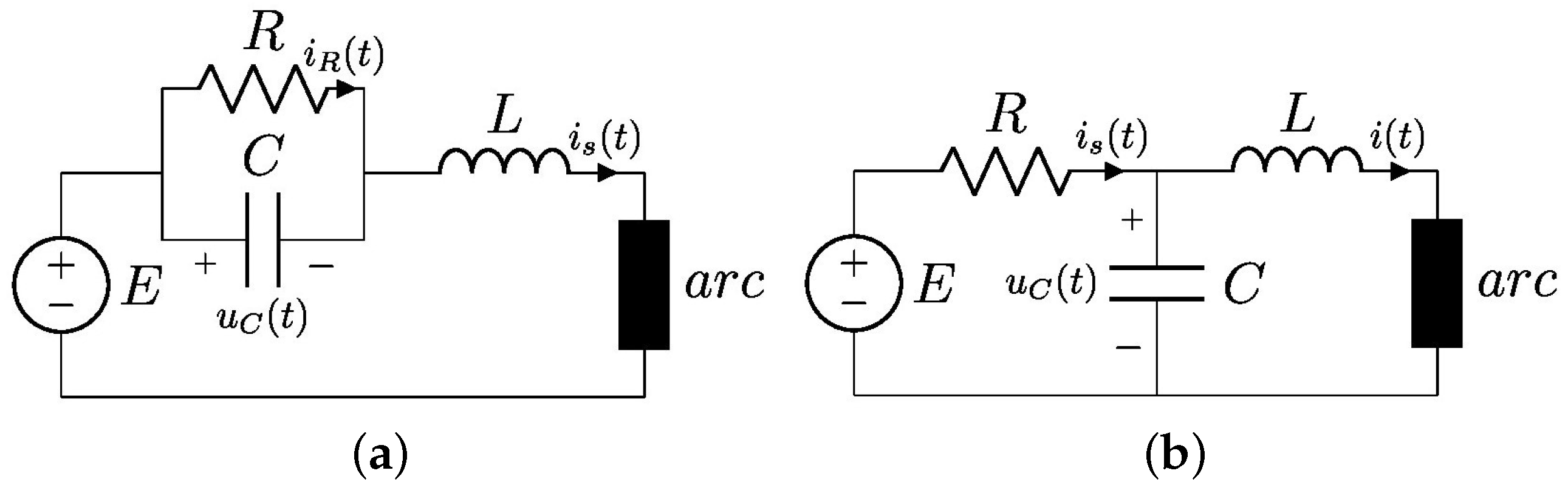
Appendix B. The Electric Arc System
Appendix C. Model of Cytosolic Calcium Oscillations
Appendix D. Sample Entropy Concept [9]
Appendix E. Computational Environment
- Figure 4a, the 0–1 test with points: 25,007 s.
- Figure 4b, the 0–1 test with points: 200,891 s.
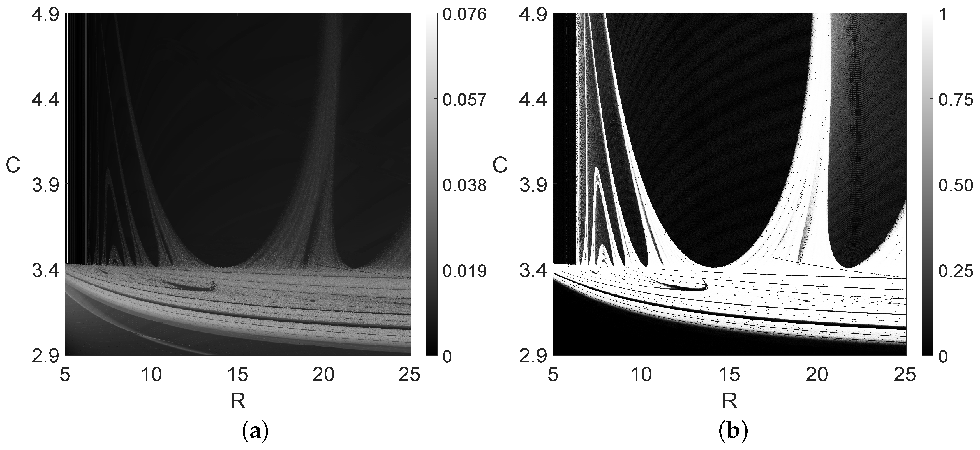
- Figure 5a, the 0–1 test with points: 4717 s.
- Figure 5b, the 0–1 test with points: 36,989 s.
- Figure 5c, the 0–1 test with points: 37,303 s.
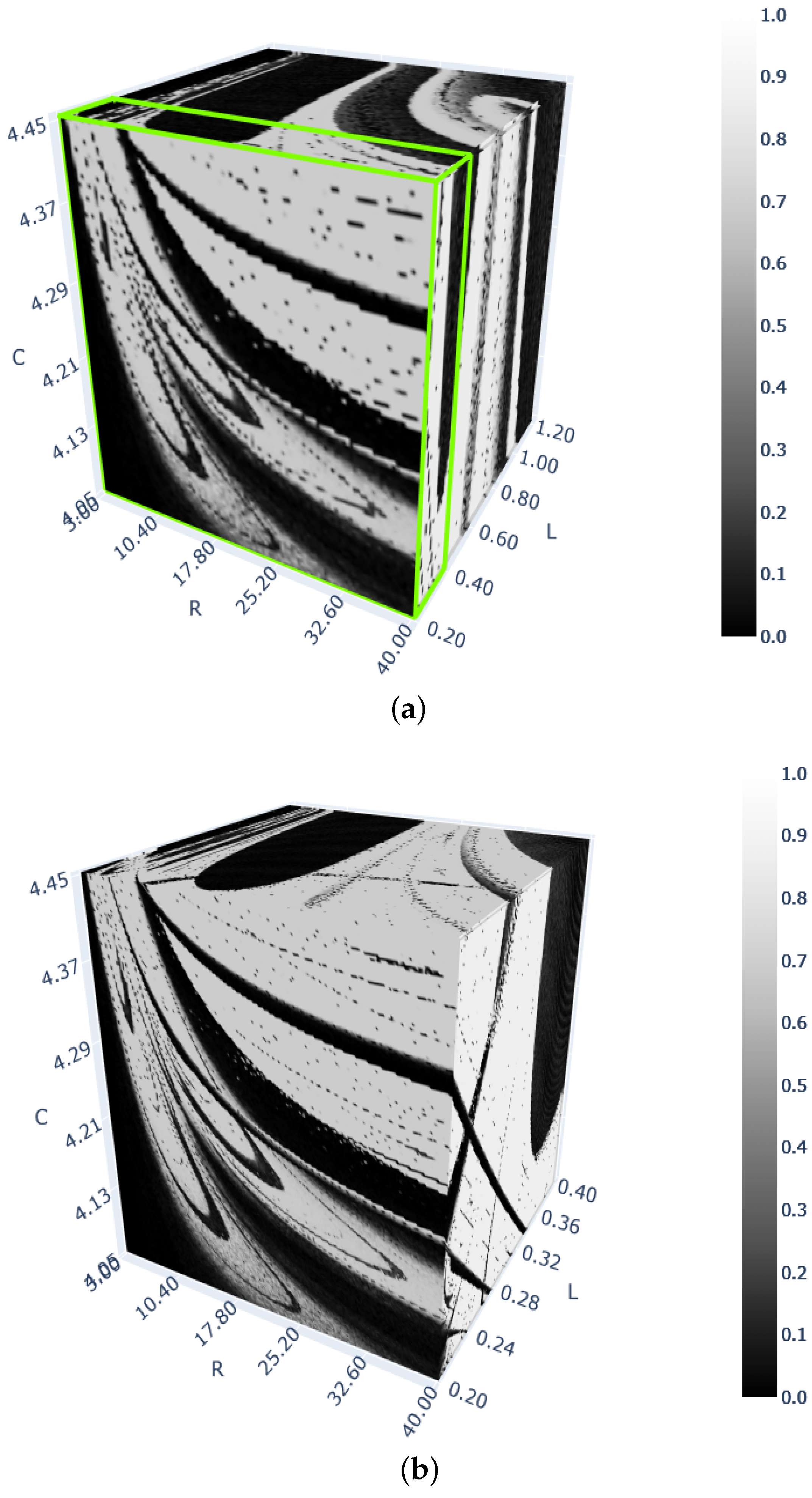
- Figure 7a, the 0–1 test diagram with points: 28,275 s.
- Figure 7b, the sample entropy method with points: 65,212 s.
- Figure 7c, the sample entropy method with points: 477,603 s.
References
- Zhou, S.; Wang, X.Y. Simple estimation method for the largest Lyapunov exponent of continuous fractional-order differential equations. Phys. A Stat. Mech. Its Appl. 2021, 653, 125478. [Google Scholar] [CrossRef]
- Gottwald, G.A.; Melbourne, I. A new test for chaos in deterministic systems. Proc. R. Soc. Lond. 2003, 460, 603–611. [Google Scholar] [CrossRef]
- Gottwald, G.A.; Melbourne, I. Testing for chaos in deterministic systems with noise. Phys. D Nonlinear Phenom. 2005, 212, 100–110. [Google Scholar] [CrossRef]
- Gottwald, G.A.; Melbourne, I. On the implementation of the 0–1 test for chaos. SIAM J. Appl. Dyn. Syst. 2009, 8, 129–145. [Google Scholar] [CrossRef]
- Melosik, M.; Marszalek, W. On the 0–1 test for chaos in continuous systems. Bull. Pol. Acad. Sci. Tech. Sci. 2016, 64, 521–528. [Google Scholar] [CrossRef]
- Walczak, M.; Marszalek, W.; Sadecki, J. Using the 0–1 test for chaos in nonlinear continuous systems with two varying parameters: Parallel computations. IEEE Access 2019, 7, 154375–154385. [Google Scholar] [CrossRef]
- Richman, J.S.; Lake, D.E.; Moorman, J.R. Sample entropy. Methods Enzymol. 2005, 384, 172–184. [Google Scholar]
- Marszalek, W.; Walczak, M.; Sadecki, J. Time series identification in the oscillatory calcium models: The 0–1 test approach with two varying parameters. In Proceedings of the 2020 59th IEEE Conference on Decision and Control, CDC, Jeju Island, Republic of Korea, 14–18 December 2020; pp. 5125–5132. [Google Scholar]
- Marszalek, W.; Walczak, M.; Sadecki, J. Two-parameter 0–1 test for chaos and sample entropy bifurcation diagrams for nonlinear oscillating systems. IEEE Access 2021, 9, 22679–22687. [Google Scholar] [CrossRef]
- Costa, M.; Goldberger, A.L.; Peng, C.-K. Multiscale entropy analysis of biological signals. Phys. Rev. E Stat. Phys. Plasmas Fluids Relat. Interdiscip. Top. 2005, 71, 021906. [Google Scholar] [CrossRef]
- Bhavsar, R.; Helian, N.; Sun, T.; Davey, N.; Steffert, T.; Mayor, D. Efficient methods for calculating sample entropy in time series data analysis. Procedia Comput. Sci. 2018, 145, 97–104. [Google Scholar] [CrossRef]
- Martinez-Cagigal, V. Sample Entropy. Mathworks. Available online: https://www.mathworks.com/matlabcentral/fileexchange/69381-sample-entropy (accessed on 15 February 2024).
- Laut, I.; Räth, C. Surrogate-assisted network analysis of nonlinear time series. Chaos 2016, 26, 103108. [Google Scholar] [CrossRef] [PubMed]
- Marszalek, W.; Hassona, S. New bifurcation diagrams based on hypothesis testing: Pseudo-periodic surrogates with correlation dimension as discriminating statistic. Mech. Syst. Signal Process. 2023, 138, 109879. [Google Scholar] [CrossRef]
- Schreiber, T.; Schmitz, A. Surrogate time series. Phys. D Nonlinear Phenom. 2000, 142, 346–382. [Google Scholar] [CrossRef]
- Lancaster, G.; Iatsenko, D.; Pidde, A.; Ticcinelli, V.; Stefanovska, A. Surrogate data for hypothesis testing of physical systems. Phys. Rep. 2018, 748, 1–60. [Google Scholar] [CrossRef]
- Small, M.; Yu, D.; Harrison, R.G. Surrogate test for pseudoperiodic time series data. Phys. Rev. Lett. 2001, 87, 188101. [Google Scholar] [CrossRef]
- Hassona, S.; Marszalek, W.; Sadecki, J. Time series classification and creation of 2D bifurcation diagrams in nonlinear dynamical systems using supervised machine learning methods. Appl. Soft Comput. 2021, 113, 107874. [Google Scholar] [CrossRef]
- Pentegov, I.V.; Sydorets, V.N. Comparative analysis of models of dynamic welding arc. Paton Weld. J. 2015, 12, 45–48. [Google Scholar] [CrossRef]
- Marszalek, W.; Sadecki, J. 2D bifurcations and chaos in nonlinear circuits: A parallel computational approach. In Proceedings of the 15th International Conference on Synthesis, Modeling, Analysis and Simulation Methods and Applications to Circuit Design (SMACD), Prague, Czech Republic, 2–5 July 2018; pp. 297–300. [Google Scholar]
- Marszalek, W.; Sadecki, J. Parallel computing of 2-D bifurcation diagrams in circuits with electric arcs. IEEE Trans. Plasma Sci. 2019, 47, 706–713. [Google Scholar] [CrossRef]
- Melosik, W.; Marszalek, W. Trojan attack on the initialization of pseudo-random bit generators using synchronization of chaotic input sources. IEEE Access 2021, 9, 161846–161853. [Google Scholar] [CrossRef]
- Marhl, M.; Haberichter, T.; Brumen, M.; Heinrich, R. Complex calcium oscillations and the role of mitochondria and cytosolic proteins. BioSystems 2000, 57, 75–86. [Google Scholar] [CrossRef]
- Grubelnick, V.; Larseb, A.Z.; Kummer, U.; Olsenb, L.F.; Marhl, M. Mitochondria regulate the amplitude of simple and complex calcium oscillations. Biophys. Chem. 2001, 94, 59–74. [Google Scholar] [CrossRef] [PubMed]
- Ji, Q.-B.; Lu, Q.-S.; Yang, Z.-Q.; Duan, L.-X. Bursting Ca2+ oscillations and synchronization in coupled cells. Chin. Phys. Lett. 2008, 25, 3879–3882. [Google Scholar]
- Li, X.; Zhanga, S.; Liu, X.; Wang, X.; Zhou, A.; Liu, P. Dynamic analysis on the calcium oscillation model considering the influences of mitochondria. BioSystems 2018, 163, 36–46. [Google Scholar] [CrossRef] [PubMed]
- Lampartová, A.; Lampart, M. Exploring diverse trajectory patterns in nonlinear dynamic systems. Chaos Solitons Fractals 2024, 182, 114863. [Google Scholar] [CrossRef]
- Marszalek, W.; Walczak, M.; Sadecki, J. Testing deterministic chaos: Incorrect results of the 0–1 test and how to avoid them. IEEE Access 2019, 7, 183245–183251. [Google Scholar] [CrossRef]


Disclaimer/Publisher’s Note: The statements, opinions and data contained in all publications are solely those of the individual author(s) and contributor(s) and not of MDPI and/or the editor(s). MDPI and/or the editor(s) disclaim responsibility for any injury to people or property resulting from any ideas, methods, instructions or products referred to in the content. |
© 2024 by the authors. Licensee MDPI, Basel, Switzerland. This article is an open access article distributed under the terms and conditions of the Creative Commons Attribution (CC BY) license (https://creativecommons.org/licenses/by/4.0/).
Share and Cite
Marszalek, W.; Walczak, M. Bifurcation Diagrams of Nonlinear Oscillatory Dynamical Systems: A Brief Review in 1D, 2D and 3D. Entropy 2024, 26, 770. https://doi.org/10.3390/e26090770
Marszalek W, Walczak M. Bifurcation Diagrams of Nonlinear Oscillatory Dynamical Systems: A Brief Review in 1D, 2D and 3D. Entropy. 2024; 26(9):770. https://doi.org/10.3390/e26090770
Chicago/Turabian StyleMarszalek, Wieslaw, and Maciej Walczak. 2024. "Bifurcation Diagrams of Nonlinear Oscillatory Dynamical Systems: A Brief Review in 1D, 2D and 3D" Entropy 26, no. 9: 770. https://doi.org/10.3390/e26090770