
Improving Transmission Line Fault Diagnosis Based on EEMD and Power Spectral Entropy


Abstract
1. Introduction
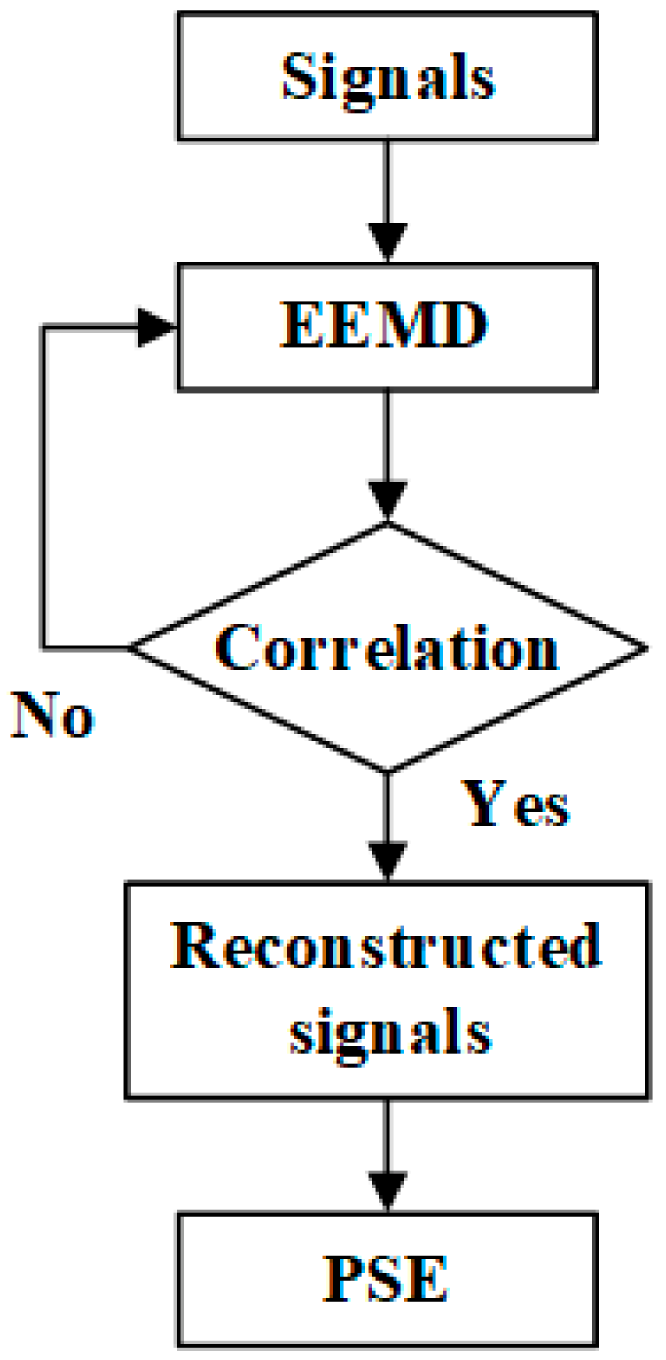
2. Method
2.1. Ensemble Empirical Mode Decomposition
- (a)
- The target data is added to the white noise sequence.
- (b)
- The target data with added white noise is decomposed into intrinsic mode functions (IMFs). Each IMF is expressed as
- (c)
- A different white noise sequence is added each time and repeats steps (a) and (b).
- (d)
- The mean of each IMF obtained by decomposition is taken as the final result defined as
2.2. Power Spectral Entropy
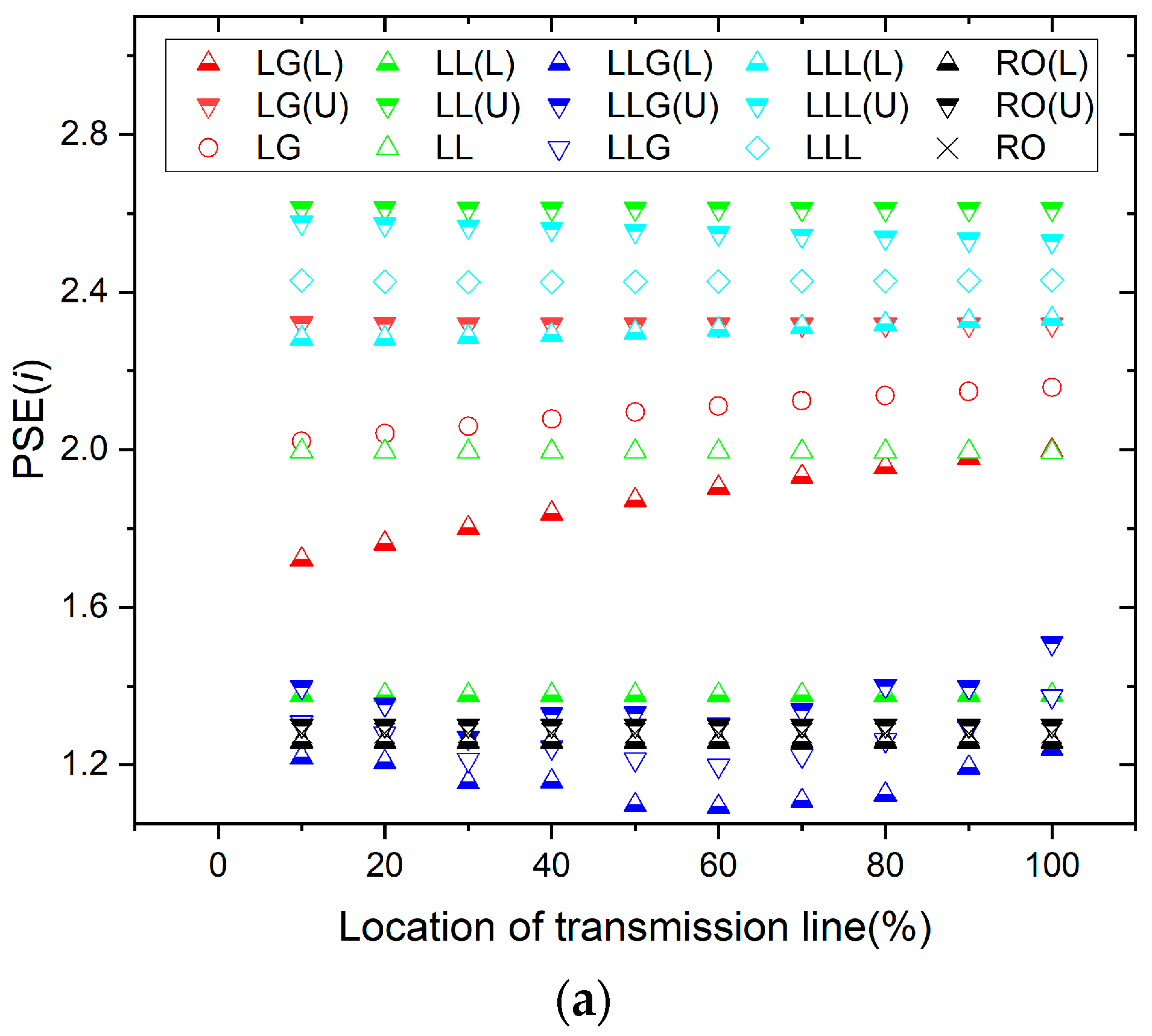
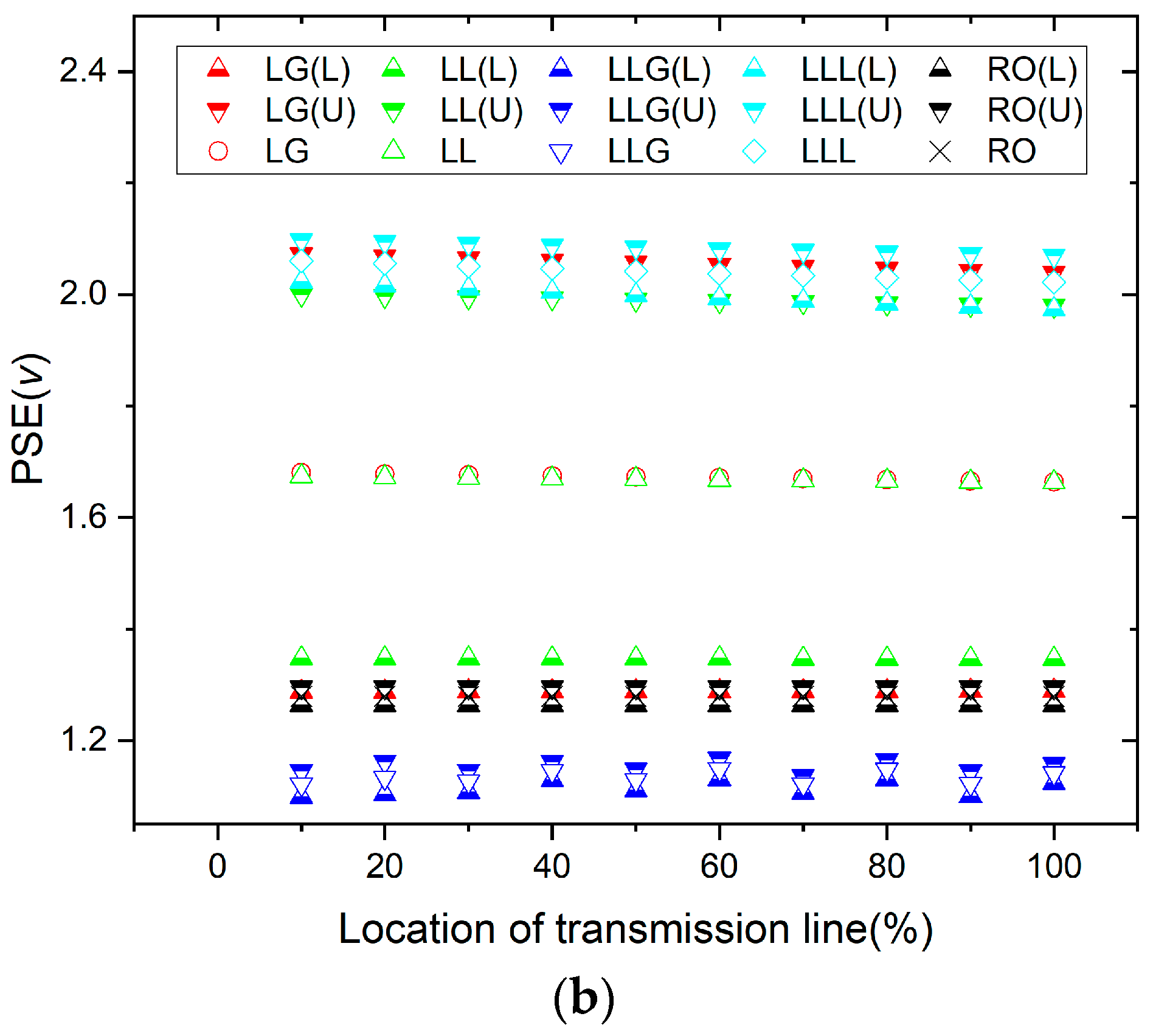
3. Results
3.1. LG Fault
3.2. LL Fault
3.3. LLG Fault
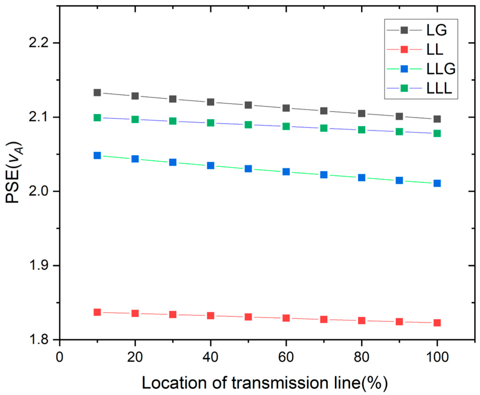
3.4. LLL Fault
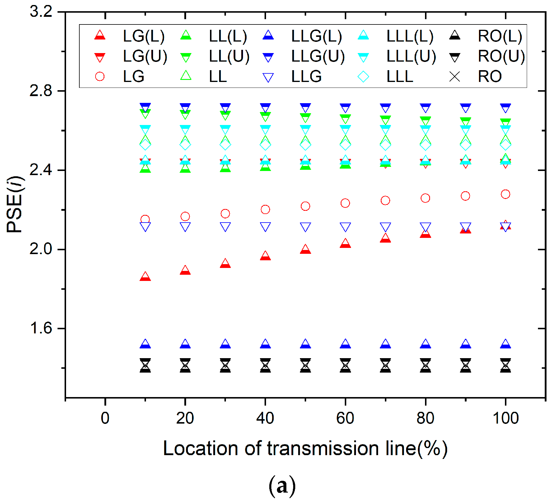
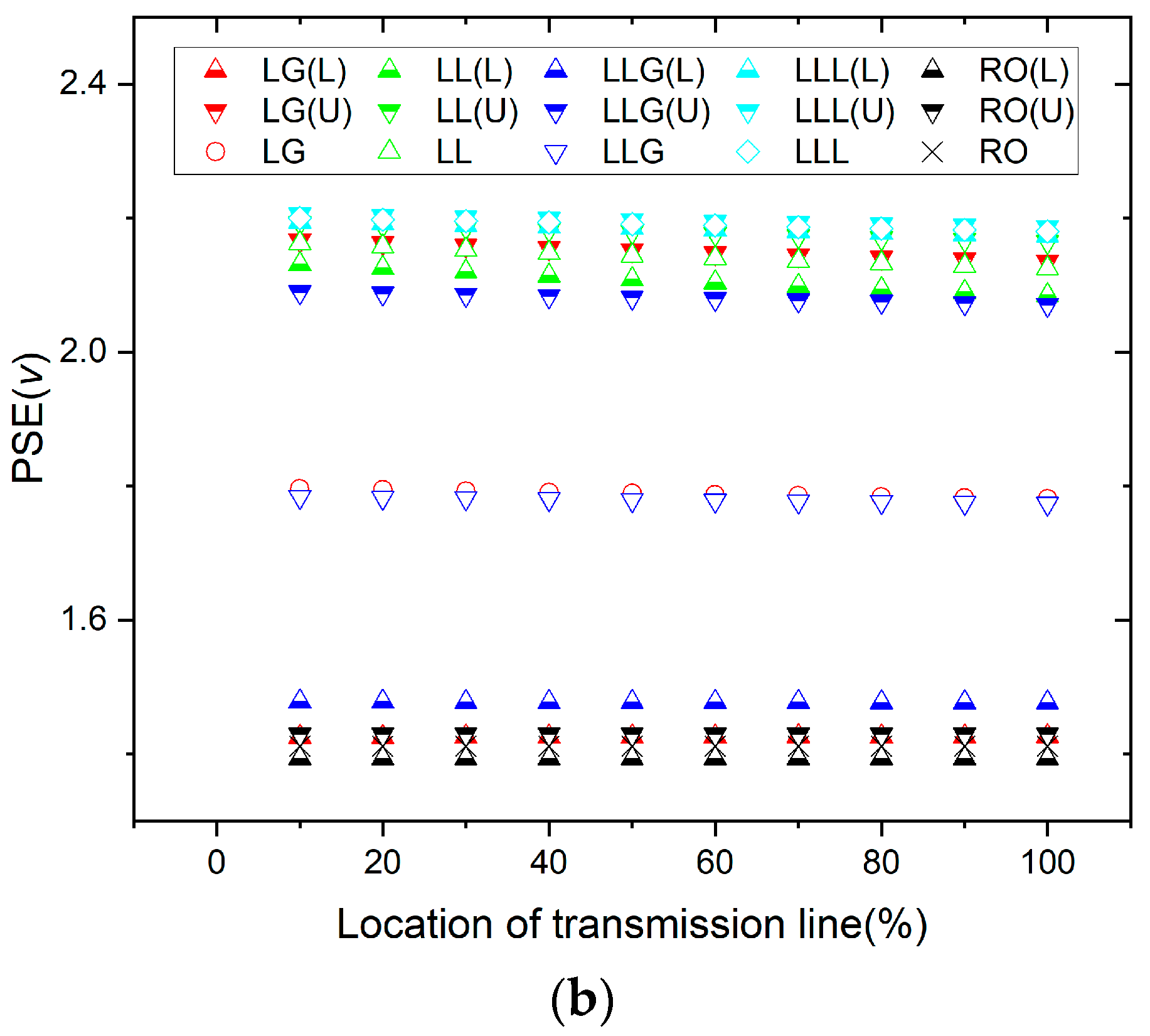
4. Discussion
5. Conclusions
Author Contributions
Funding
Institutional Review Board Statement
Data Availability Statement
Conflicts of Interest
References
- Tleis, N. Power Systems Modelling and Fault Analysis, 2nd ed.; Academic Press: New York, NY, USA, 2019; pp. 1–14. [Google Scholar]
- Demirci, M.; Gözde, H. Improvement of power transformer fault diagnosis by using sequential Kalman filter sensor fusion. Int. J. Elect. Power & Energy Syst. 2023, 149, 109038. [Google Scholar]
- Chowdhury, T.; Chakrabarti, A. Power Transmission System Analysis Against Faults and Attacks; CRC Press: Boca Raton, FL, USA, 2019. [Google Scholar]
- Geng, Q.; Sun, H. A Storage-Based Fixed-Time Frequency Synchronization Method for Improving Transient Stability and Resilience of Smart Grid. IEEE Trans. Smart Grid 2023, 14, 4799–4815. [Google Scholar] [CrossRef]
- Hsu, W.T.; Huang, C.W. Analysis of Symmetrical and Unsymmetrical Faults Using the EEMD and Scale-Dependent Intrinsic Entropies. Fluct. Noise Lett. 2022, 21, 1–14. [Google Scholar] [CrossRef]
- Yang, N.C.; Yang, J.M. Fault Classification in Distribution Systems Using Deep Learning with Data Preprocessing Methods Based on Fast Dynamic Time Warping and Short-Time Fourier Transform. IEEE Access 2023, 11, 63612–63622. [Google Scholar] [CrossRef]
- Altaie, A.S.; Majeed, A.A. Fault Detection on Power Transmission Line Based on Wavelet Transform and Scalogram Image Analysis. Energies 2023, 16, 7914. [Google Scholar] [CrossRef]
- Priyadarshini, M.S.; Krishna, D. Significance of Harmonic Filters by Computation of Short-Time Fourier Transform-Based Time–Frequency Representation of Supply Voltage. Energies 2023, 16, 2194. [Google Scholar] [CrossRef]
- Li, Q.; Luo, H. Incipient Fault Detection in Power Distribution System: A Time–Frequency Embedded Deep-Learning-Based Approach. IEEE Trans. Instrum. Meas. 2023, 72, 2507914. [Google Scholar] [CrossRef]
- Ribeiro, P.F.; Duque, C.A. Power Systems Signal Processing for Smart Grids; John Wiley & Sons: Hoboken, NJ, USA, 2015. [Google Scholar]
- Yang, Y.; Zhang, Q. Fault Location Method of Multi-Terminal Transmission Line Based on Fault Branch Judgment Matrix. Appl. Sci. 2023, 13, 1174. [Google Scholar] [CrossRef]
- Shakiba, F.M.; Azizi, S.M. Application of machine learning methods in fault detection and classification of power transmission lines: A survey. Artif. Intell. Rev. 2023, 56, 5799–5836. [Google Scholar] [CrossRef]
- Xi, Y.; Zhang, W. Transmission line fault detection and classification based on SA-MobileNetV3. Energy Rep. 2023, 9, 955–968. [Google Scholar] [CrossRef]
- Grainger, J.J.; Stevenson, W.D. Power System Analysis, 2nd ed.; McGraw-Hill: New York, NY, USA, 2021. [Google Scholar]
- Huang, N.E.; Zhang, J.; Wu, Z.H. Adaptive Analysis Method for Nonlinear and Non-Stationary Data; China Science Publishing & Media Ltd.: Beijing, China, 2024. (In Chinese) [Google Scholar]
- Huang, N.E.; Shen; Samuel, S.P. Hilbert-Huang Transform and ITS Applications, 2nd ed.; World Scientific: Singapore, 2014. [Google Scholar]
- Zhao, S.; Ma, L.; Xu, L.; Liu, M.; Chen, X. A Study of Fault Signal Noise Reduction Based on Improved CEEMDAN-SVD. Appl. Sci. 2023, 13, 10713. [Google Scholar] [CrossRef]
- Ding, S.F.; Zhang, Z.C.; Guo, L.L.; Sun, Y.T. An optimized twin support vector regression algorithm enhanced by ensemble empirical mode decomposition and gated recurrent unit. Inf. Sci. 2022, 598, 101–125. [Google Scholar] [CrossRef]
- Zhao, Y.; Cheng, X. Cross-entropy based importance sampling for composite systems reliability evaluation with consideration of multivariate dependence. Int. J. Elect. Power & Energy Syst. 2023, 157, 109874. [Google Scholar]
- Zheng, Z.; Xin, G. Fault Feature Extraction of Hydraulic Pumps Based on Symplectic Geometry Mode Decomposition and Power Spectral Entropy. Entropy 2019, 21, 476. [Google Scholar] [CrossRef] [PubMed]
- Dong, J.; Song, Z. Identification of Critical Links Based on Electrical Betweenness and Neighborhood Similarity in Cyber-Physical Power Systems. Entropy 2024, 26, 85. [Google Scholar] [CrossRef]
- Ribeiro, M.; Henriques, T.; Castro, L.; Souto, A.; Antunes, L.; Costa-Santos, C.; Teixeira, A. The Entropy Universe. Entropy 2021, 23, 222. [Google Scholar] [CrossRef]
- Tsallis, C. Entropy. Encyclopedia 2022, 2, 264–300. [Google Scholar] [CrossRef]
- Mittal, M.; Shah, R.R.; Roy, S. Cognitive Computing for Human-Robot Interaction Principles and Practices; Academic Press: San Diego, CA, USA, 2021. [Google Scholar]
- Helakari, H.; Kananen, J.; Huotari, N.; Raitamaa, L.; Tuovinen, T.; Borchardt, V.; Rasila, A.; Raatikainen, V.; Starck, T.; Hautaniemi, T.; et al. Spectral entropy indicates electrophysiological and hemodynamic changes in drug-resistant epilepsy—A multimodal MREG study. Neuroimage Clin. 2019, 22, 101763. [Google Scholar] [CrossRef]
- Kokes, M.G.; Gibson, J.D. Frontiers in Entropy Across the Disciplines Panorama of Entropy: Theory, Computation, and Applications; World Scientific Publishing: Singapore, 2022; pp. 331–351. [Google Scholar]
- Acharya, U.R.; Fujita, H.; Sudarshan, V.K.; Bhat, S.; Koh, J.E.W. Application of entropies for automated diagnosis of epilepsy using EEG signals: A review. Knowl.-Based Syst. 2015, 88, 85–96. [Google Scholar] [CrossRef]
- Dai, Y.; Zhang, H. Complexity–entropy causality plane based on power spectral entropy for complex time series. Phys. A 2018, 509, 501–514. [Google Scholar] [CrossRef]
- Zeng, X.; Xiong, X. Grid Fault Diagnosis Based on Information Entropy and Multi-source Information Fusion. Intl. J. Electron. Telecommun. 2021, 67, 143–148. [Google Scholar] [CrossRef]
- Wu, Z.H.; Huang, N.E. Ensemble Empirical Mode Decomposition: A Noise-Assisted Data Analysis Method. Adv. Adapt. Data Anal. 2009, 1, 1–41. [Google Scholar] [CrossRef]
- Huang, N.E.; Wu, Z.H.; Pinzon, J.E. Reductions of noise and uncertainty in annual global surface temperature anomaly data. Adv. Adapt. Data Anal. 2009, 1, 447–460. [Google Scholar] [CrossRef]
- Li, M.; Liu, X. Infrasound signal classification based on spectral entropy and support vector machine. Appl. Acoust. 2016, 113, 116–120. [Google Scholar] [CrossRef]
- Cao, C.; Liu, M. Mechanical Fault Diagnosis of High Voltage Circuit Breakers Utilizing VMD Based on Improved Time Segment Energy Entropy and a New Hybrid Classifier. IEEE Access 2020, 8, 177767–177781. [Google Scholar] [CrossRef]
- Yan, J.; Peng, M. Fault Diagnosis of Grounding Grids Based on Information Entropy and Evidence Fusion. Proc. CSU-EPSA 2017, 29, 8–13. [Google Scholar]
- Rucco, M.; Gonzalez-Diaz, R. A new topological entropy-based approach for measuring similarities among piecewise linear functions. Signal Process 2017, 134, 130–138. [Google Scholar] [CrossRef]


| PSE | iA | iB | iC | vA | vB | vC |
|---|---|---|---|---|---|---|
| 10% | 2.46468 | 1.88660 | 2.09875 | 2.22387 | 1.59409 | 1.57016 |
| 20% | 2.46321 | 1.91518 | 2.11969 | 2.21987 | 1.59319 | 1.56947 |
| 30% | 2.46224 | 1.95834 | 2.12055 | 2.21554 | 1.59228 | 1.56901 |
| 40% | 2.46121 | 1.98945 | 2.15431 | 2.21150 | 1.59163 | 1.56854 |
| 50% | 2.46029 | 2.02206 | 2.17150 | 2.20763 | 1.59080 | 1.56764 |
| 60% | 2.45941 | 2.05131 | 2.18770 | 2.20382 | 1.59006 | 1.56720 |
| 70% | 2.45858 | 2.07753 | 2.20272 | 2.20017 | 1.58961 | 1.56676 |
| 80% | 2.45778 | 2.10094 | 2.21650 | 2.19641 | 1.58863 | 1.56616 |
| 90% | 2.45702 | 2.12179 | 2.22905 | 2.19321 | 1.58793 | 1.56558 |
| 100% | 2.45630 | 2.14043 | 2.24043 | 2.18952 | 1.58724 | 1.56534 |
| RO | 1.42620 | 1.39136 | 1.42516 | 1.39867 | 1.40357 | 1.43162 |
| PSE | iA | iB | iC | vA | vB | vC |
|---|---|---|---|---|---|---|
| 10% | 2.63014 | 2.63275 | 2.38153 | 2.14312 | 2.19759 | 2.14543 |
| 20% | 2.62584 | 2.62981 | 2.38130 | 2.13863 | 2.19416 | 2.13908 |
| 30% | 2.62171 | 2.62702 | 2.38553 | 2.13424 | 2.19076 | 2.13324 |
| 40% | 2.61779 | 2.62439 | 2.39203 | 2.12995 | 2.18758 | 2.12716 |
| 50% | 2.61414 | 2.62185 | 2.39975 | 2.12557 | 2.18487 | 2.12131 |
| 60% | 2.61064 | 2.61946 | 2.40797 | 2.12121 | 2.18209 | 2.11674 |
| 70% | 2.60730 | 2.61720 | 2.41631 | 2.11747 | 2.17894 | 2.11127 |
| 80% | 2.60412 | 2.61501 | 2.42458 | 2.11378 | 2.17626 | 2.10608 |
| 90% | 2.60108 | 2.61291 | 2.43249 | 2.11025 | 2.17356 | 2.10163 |
| 100% | 2.59817 | 2.61091 | 2.44001 | 2.10642 | 2.17044 | 2.09671 |
| RO | 1.42620 | 1.39136 | 1.42516 | 1.39867 | 1.40357 | 1.43162 |
| PSE | iA | iB | iC | vA | vB | vC |
|---|---|---|---|---|---|---|
| 10% | 2.47218 | 2.46368 | 1.42445 | 1.93754 | 1.98244 | 1.43166 |
| 20% | 2.47196 | 2.46345 | 1.42444 | 1.93591 | 1.98043 | 1.43162 |
| 30% | 2.47173 | 2.46322 | 1.42443 | 1.93435 | 1.97870 | 1.43164 |
| 40% | 2.47151 | 2.46299 | 1.42442 | 1.93278 | 1.97732 | 1.43168 |
| 50% | 2.47128 | 2.46276 | 1.42440 | 1.93139 | 1.97517 | 1.43169 |
| 60% | 2.47106 | 2.46254 | 1.42440 | 1.92984 | 1.97354 | 1.43166 |
| 70% | 2.47084 | 2.46232 | 1.42439 | 1.92828 | 1.97158 | 1.43175 |
| 80% | 2.47061 | 2.46209 | 1.42439 | 1.92662 | 1.96983 | 1.43167 |
| 90% | 2.47038 | 2.46187 | 1.42438 | 1.92517 | 1.96805 | 1.43167 |
| 100% | 2.47014 | 2.46164 | 1.42437 | 1.92360 | 1.96601 | 1.43164 |
| RO | 1.42620 | 1.39136 | 1.42516 | 1.39867 | 1.40357 | 1.43162 |
| PSE | iA | iB | iC | vA | vB | vC |
|---|---|---|---|---|---|---|
| 10% | 2.43759 | 2.55454 | 2.59627 | 2.19564 | 2.19793 | 2.20611 |
| 20% | 2.43744 | 2.55432 | 2.59616 | 2.19327 | 2.19553 | 2.20389 |
| 30% | 2.43731 | 2.55411 | 2.59605 | 2.19085 | 2.19335 | 2.20176 |
| 40% | 2.43717 | 2.55388 | 2.59594 | 2.18862 | 2.19149 | 2.19966 |
| 50% | 2.43701 | 2.55368 | 2.59584 | 2.18638 | 2.18901 | 2.19778 |
| 60% | 2.43687 | 2.55346 | 2.59575 | 2.18405 | 2.18708 | 2.19566 |
| 70% | 2.43671 | 2.55323 | 2.59564 | 2.18174 | 2.18456 | 2.19362 |
| 80% | 2.43656 | 2.55300 | 2.59555 | 2.17934 | 2.18218 | 2.19150 |
| 90% | 2.43643 | 2.55279 | 2.59545 | 2.17732 | 2.17973 | 2.18954 |
| 100% | 2.43629 | 2.55257 | 2.59534 | 2.17516 | 2.17741 | 2.18740 |
| RO | 1.42620 | 1.39136 | 1.42516 | 1.39867 | 1.40357 | 1.43162 |
Disclaimer/Publisher’s Note: The statements, opinions and data contained in all publications are solely those of the individual author(s) and contributor(s) and not of MDPI and/or the editor(s). MDPI and/or the editor(s) disclaim responsibility for any injury to people or property resulting from any ideas, methods, instructions or products referred to in the content. |
© 2024 by the authors. Licensee MDPI, Basel, Switzerland. This article is an open access article distributed under the terms and conditions of the Creative Commons Attribution (CC BY) license (https://creativecommons.org/licenses/by/4.0/).
Share and Cite
Chen, Y.-B.; Cui, H.-S.; Huang, C.-W.; Hsu, W.-T. Improving Transmission Line Fault Diagnosis Based on EEMD and Power Spectral Entropy. Entropy 2024, 26, 806. https://doi.org/10.3390/e26090806
Chen Y-B, Cui H-S, Huang C-W, Hsu W-T. Improving Transmission Line Fault Diagnosis Based on EEMD and Power Spectral Entropy. Entropy. 2024; 26(9):806. https://doi.org/10.3390/e26090806
Chicago/Turabian StyleChen, Yuan-Bin, Hui-Shan Cui, Chia-Wei Huang, and Wei-Tai Hsu. 2024. "Improving Transmission Line Fault Diagnosis Based on EEMD and Power Spectral Entropy" Entropy 26, no. 9: 806. https://doi.org/10.3390/e26090806
APA StyleChen, Y.-B., Cui, H.-S., Huang, C.-W., & Hsu, W.-T. (2024). Improving Transmission Line Fault Diagnosis Based on EEMD and Power Spectral Entropy. Entropy, 26(9), 806. https://doi.org/10.3390/e26090806