
Dynamical Complexity in Geomagnetically Induced Current Activity Indices Using Block Entropy

 , ,
, ,  , , and
Abstract
:1. Introduction
2. Materials and Methods
2.1. GIC Index
2.2. Block Entropy
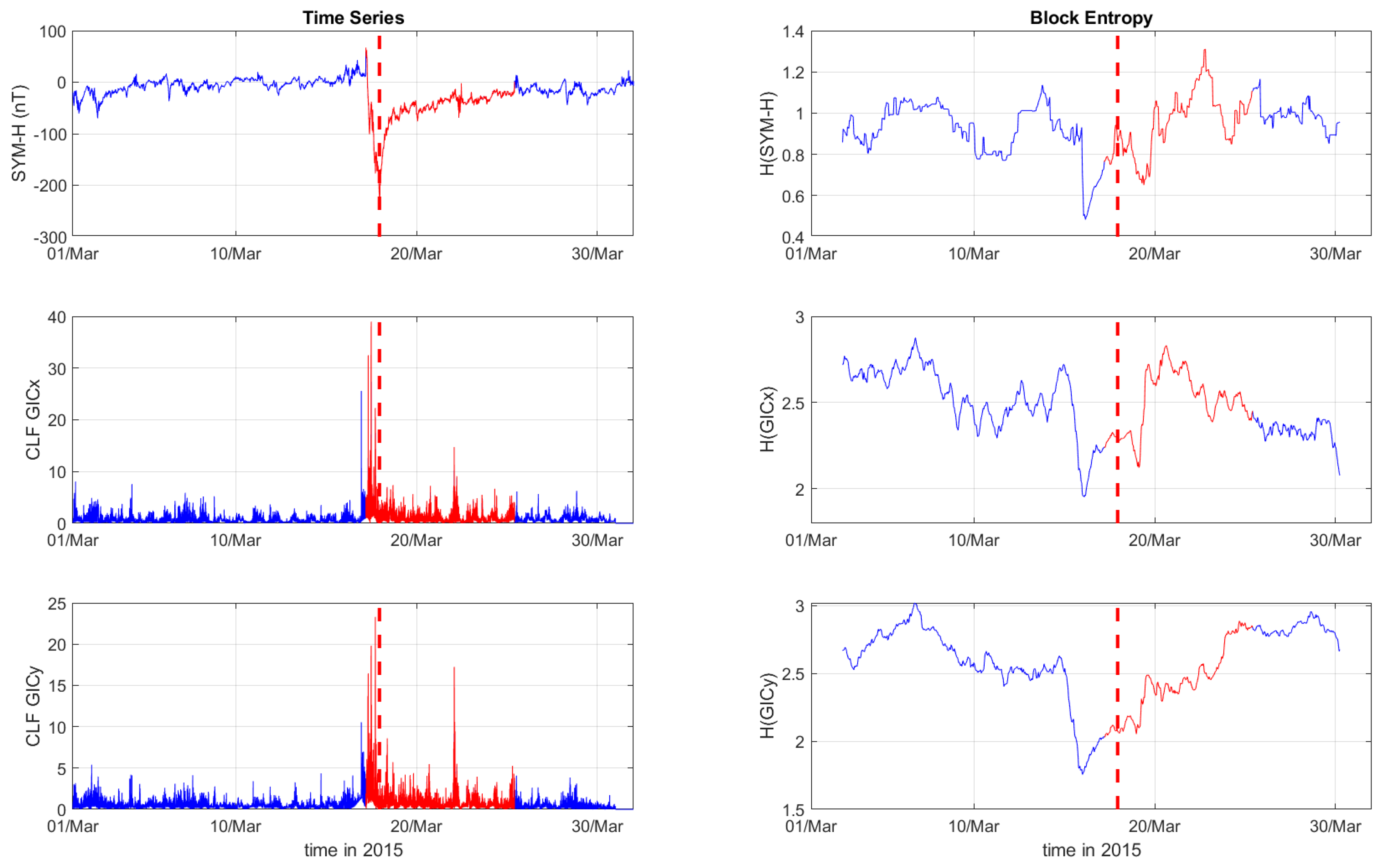
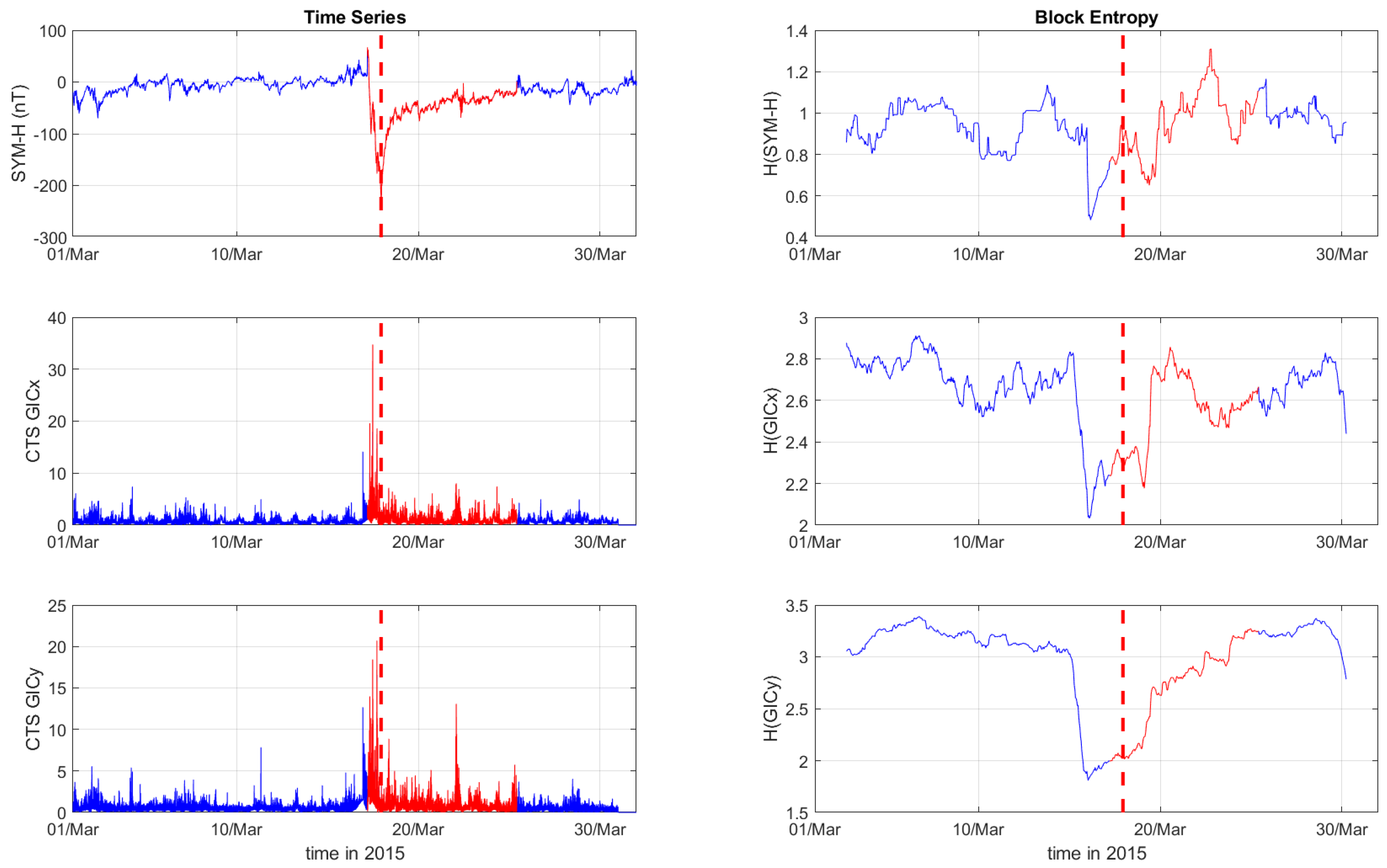
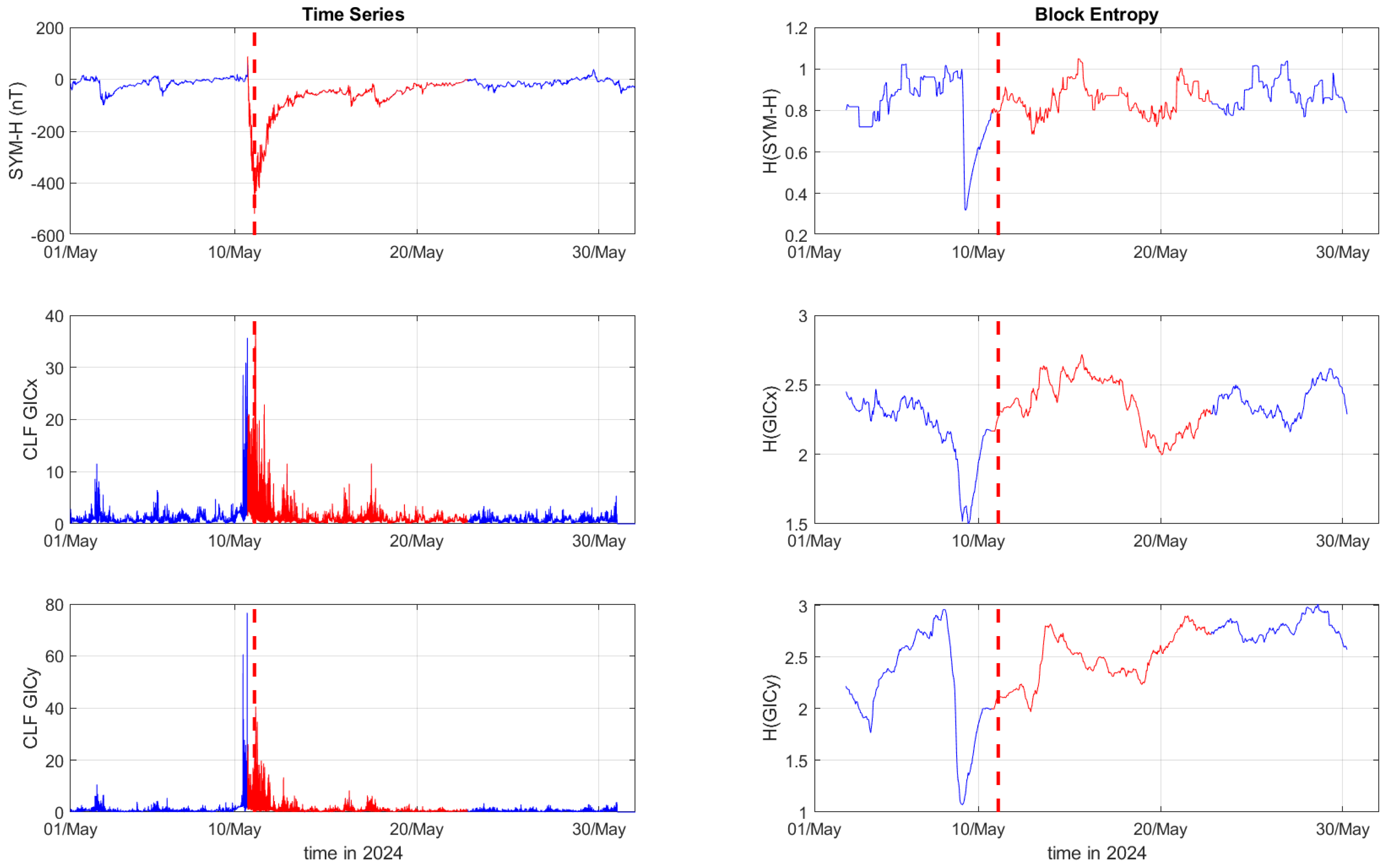
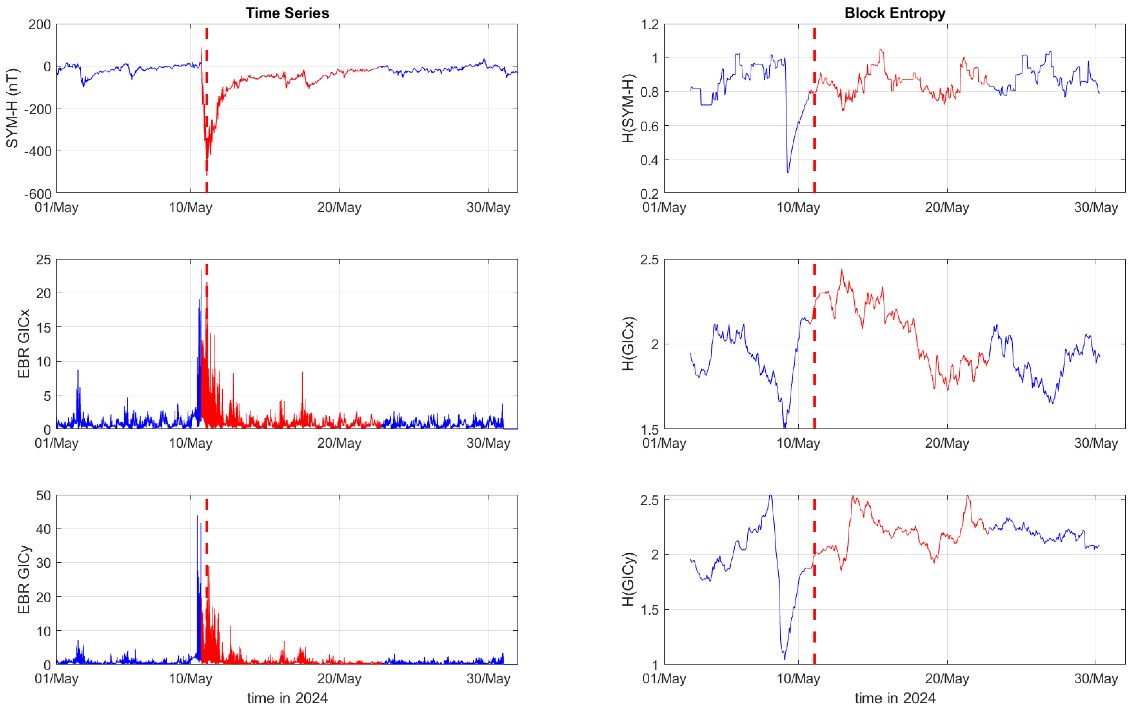
3. Results
4. Discussion
5. Conclusions
Author Contributions
Funding
Institutional Review Board Statement
Informed Consent Statement
Data Availability Statement
Acknowledgments
Conflicts of Interest
References
- Pirjola, R. Geomagnetically induced currents during magnetic storms. IEEE Trans. Plasma Sci. 2000, 28, 1867–1873. [Google Scholar] [CrossRef]
- Daglis, I.A.; Baker, D.N.; Galperin, Y.; Kappenman, J.G.; Lanzerotti, L.J. Technological impacts of space storms: Outstanding issues. Eos Trans. Am. Geophys. Union 2001, 82, 585, 591–592. [Google Scholar] [CrossRef]
- Daglis, I.A. Geospace storm dynamics. In Effects of Space Weather on Technology Infrastructure. NATO Science Series II: Mathematics, Physics and Chemistry; Daglis, I.A., Ed.; Springer: Dordrecht, The Netherlands, 2004; pp. 27–42. [Google Scholar] [CrossRef]
- Baker, D.N.; Daly, E.; Daglis, I.A.; Kappenman, J.G.; Panasyuk, M. Effects of Space Weather on Technology Infrastructure. Space Weather 2004, 2. [Google Scholar] [CrossRef]
- Ngwira, C.M.; Pulkkinen, A.; McKinnell, L.A.; Cilliers, P.J. Improved modeling of geomagnetically induced currents in the South African power network. Space Weather. 2008, 6, S11004. [Google Scholar] [CrossRef]
- Matandirotya, E.; Cilliers, P.J.; Van Zyl, R.R. Modeling geomagnetically induced currents in the South African power transmission network using the finite element method. Space Weather 2015, 13, 185–195. [Google Scholar] [CrossRef]
- Viljanen, A.; Pirjola, R. Geomagnetically induced currents in the Finnish high-voltage power system. Surv. Geophys. 1994, 15, 383–408. [Google Scholar] [CrossRef]
- Pirjola, R.; Pulkkinen, A.; Viljanen, A. Studies of space weather effects on the Finnish natural gas pipeline and on the Finnish high-voltage power system. Adv. Space Res. 2003, 31, 795–805. [Google Scholar] [CrossRef]
- Torta, J.M.; Marsal, S.; Quintana, M. Assessing the hazard from geomagnetically induced currents to the Spanish entire high-voltage power network in Spain. Earth Planets Space 2014, 66, 87. [Google Scholar] [CrossRef]
- Tozzi, R.; De Michelis, P.; Coco, I.; Giannattasio, F. A preliminary risk assessment of geomagnetically induced currents over the Italian territory. Space Weather 2019, 17, 46–58. [Google Scholar] [CrossRef]
- Balasis, G.; Balikhin, M.A.; Chapman, S.C.; Consolini, G.; Daglis, I.A.; Donner, R.V.; Kurths, J.; Paluš, M.; Runge, J.; Tsurutani, B.T.; et al. Complex Systems Methods Characterizing Nonlinear Processes in the Near-Earth Electromagnetic Environment: Recent Advances and Open Challenges. Space Sci. Rev. 2023, 219, 38. [Google Scholar] [CrossRef]
- Wing, S.; Balasis, G. Preface: Information theory and machine learning for geospace research. Adv. Space Res. 2024, 74, 6249–6251. [Google Scholar] [CrossRef]
- Papadimitriou, C.; Balasis, G.; Boutsi, A.Z.; Daglis, I.A.; Giannakis, O.; Anastasiadis, A.; De Michelis, P.; Consolini, G. Dynamical Complexity of the 2015 St. Patrick’s Day Magnetic Storm at Swarm Altitudes Using Entropy Measures. Entropy 2020, 22, 574. [Google Scholar] [CrossRef] [PubMed]
- De Michelis, P.; Pignalberi, A.; Consolini, G.; Coco, I.; Tozzi, R.; Pezzopane, M.; Giannattasio, F.; Balasis, G. On the 2015 St. Patrick’s Storm Turbulent State of the Ionosphere: Hints From the Swarm Mission. J. Geophys. Res. Space Phys. 2020, 125, e2020JA027934. [Google Scholar] [CrossRef]
- Marshall, R.A.; Waters, C.L.; Sciffer, M.D. Spectral analysis of pipe-to-soil potentials with variations of the Earth’s magnetic field in the Australian region. Space Weather 2010, 8, S05002. [Google Scholar] [CrossRef]
- Boteler, D.H.; Pirjola, R.J.; Nevanlinna, H. The effects of geomagnetic disturbances on electrical systems at the earth’s surface. Adv. Space Res. 1998, 22, 17–27. [Google Scholar] [CrossRef]
- Kappenman, J.G. An introduction to power grid impacts and vulnerabilities from space weather. In Space Storms and Space Weather Hazards. NATO Science Series (Series II: Mathematics, Physics and Chemistry; Daglis, I.A., Ed.; Springer: Dordrecht, The Netherlands, 2001; pp. 335–361. [Google Scholar] [CrossRef]
- Mayaud, P.N. Derivation, Meaning, and Use of Geomagnetic Indices. In Geophysical Monograph Series; American Geophysical Union (AGU): Washington, DC, USA, 1980. [Google Scholar] [CrossRef]
- Matzka, J.; Stolle, C.; Yamazaki, Y.; Bronkalla, O.; Morschhauser, A. The geomagnetic Kp index and derived indices of geomagnetic activity. Space Weather 2021, 19, e2020SW002641. [Google Scholar] [CrossRef]
- Tozzi, R.; Coco, I.; De Michelis, P.; Giannattasio, F. Latitudinal dependence of geomagnetically induced currents during geomagnetic storms. Ann. Geophys. 2019, 62, 448. [Google Scholar] [CrossRef]
- Boutsi, A.Z.; Balasis, G.; Dimitrakoudis, S.; Daglis, I.A.; Tsinganos, K.; Papadimitriou, C.; Giannakis, O. Investigation of the geomagnetically induced current index levels in the Mediterranean region during the strongest magnetic storms of solar cycle 24. Space Weather 2023, 21, e2022SW003122. [Google Scholar] [CrossRef]
- Pulkkinen, A.; Bernabeu, E.; Eichner, J.; Viljanen, A.; Ngwira, C. Regional-scale high-latitude extreme geoelectric fields pertaining to geomagnetically induced currents. Earth Planets Space 2015, 67, 93. [Google Scholar] [CrossRef]
- Astafyeva, E.; Zakharenkova, I.; Förster, M. Ionospheric response to the 2015 St. Patrick’s Day storm: A global multi-instrumental overview. J. Geophys. Res. Space Physics 2015, 120, 9023–9037. [Google Scholar] [CrossRef]
- Nayak, C.; Tsai, L.-C.; Su, S.-Y.; Galkin, I.A.; Tan, A.T.K.; Nofri, E.; Jamjareegulgarn, P. Peculiar features of the low-latitude and midlatitude ionospheric response to the St. Patrick’s Day geomagnetic storm of 17 March 2015. J. Geophys. Res. Space Physics 2016, 121, 7941–7960. [Google Scholar] [CrossRef]
- D’Angelo, G.; Piersanti, M.; Alfonsi, L.; Spogli, L.; Clausen, L.B.N.; Coco, I.; Li, G.; Baiqi, N. The response of high latitude ionosphere to the 2015 St. Patrick’s day storm from in situ and ground based observations. Adv. Space Res. 2018, 62, 638–650. [Google Scholar] [CrossRef]
- Tulasi Ram, S.; Veenadhari, B.; Dimri, A.P.; Bulusu, J.; Bagiya, M.; Gurubaran, S.; Parihar, N.; Remya, B.; Seemala, G.; Singh, R.; et al. Super-intense geomagnetic storm on 10–11 May 2024: Possible mechanisms and impacts. Space Weather 2024, 22, e2024SW004126. [Google Scholar] [CrossRef] [PubMed]
- Hayakawa, H.; Ebihara, Y.; Mishev, A.; Koldobskiy, S.; Kusano, K.; Bechet, S.; Yashiro, S.; Iwai, K.; Shinbori, A.; Mursula, K.; et al. The solar and geomagnetic storms in may 2024: A flash data report. Astrophys. J. 2025, 979, 49. [Google Scholar] [CrossRef]
- Spogli, L.; Alberti, T.; Bagiacchi, P.; Cafarella, L.; Cesaroni, C.; Cianchini, G.; Coco, I.; Di Mauro, D.; Ghidoni, R.; Giannattasio, F.; et al. The effects of the May 2024 Mother’s Day superstorm over the Mediterranean sector: From data to public communication. Ann. Geophys. 2024, 67, PA218. [Google Scholar] [CrossRef]
- Dungey, J.W. Interplanetary magnetic field and the auroral zones. Phys. Rev. Lett. 1961, 6, 47–48. [Google Scholar] [CrossRef]
- Papitashvili, N.E.; King, J.H. OMNI 1-min Data [SYM-H]. NASA Space Physics Data Facility. 2020. Available online: https://hpde.io/NASA/NumericalData/OMNI/HighResolutionObservations/Version1/PT1M (accessed on 8 November 2024).
- Consolini, G.; De Michelis, P.; Alberti, T.; Coco, I.; Giannattasio, F.; Tozzi, R.; Carbone, V. Intermittency and passive scalar nature of electron density fluctuations in the high-latitude ionosphere at Swarm altitude. Geophys. Res. Lett. 2020, 47, e2020GL089628. [Google Scholar] [CrossRef]
- Cagniard, L. Basic theory of the magneto-telluric method of geophysical prospecting. Geophysics 1953, 18, 605–635. [Google Scholar] [CrossRef]
- Marshall, R.A.; Smith, E.A.; Francis, M.J.; Waters, C.L.; Sciffer, M.D. A preliminary risk assessment of the Australian region power network to space weather. Space Weather 2011, 9, S10004. [Google Scholar] [CrossRef]
- Shannon, C.E. A mathematical theory of communication. Bell Syst. Tech. J. 1948, 27, 379–423. [Google Scholar] [CrossRef]
- Ebeling, W.; Nicolis, G. Word frequency and entropy of symbolic sequences: A dynamical perspective. Chaos Solitons Fractals 1992, 2, 635–650. [Google Scholar] [CrossRef]
- Nicolis, G.; Gaspard, P. Toward a probabilistic approach to complex systems. Chaos Solitons Fractals 1994, 4, 41–57. [Google Scholar] [CrossRef]
- Kappenman, J.G. An overview of the impulsive geomagnetic field disturbances and power grid impacts associated with the violent Sun-Earth connection events of 29–31 October 2003 and a comparative evaluation with other contemporary storms. Space Weather 2005, 3, S08C01. [Google Scholar] [CrossRef]
- Kappenman, J.G. Storm sudden commencement events and the associated geomagnetically induced current risks to ground-based systems at low-latitude and midlatitude locations. Space Weather 2003, 1, 1016. [Google Scholar] [CrossRef]
- Gosling, J.; Pizzo, V. Formation and evolution of corotating interaction regions and their three dimensional structure. Space Sci. Rev. 1999, 89, 21–52. [Google Scholar] [CrossRef]
- Hejda, P.; Bochníček, J. Geomagnetically induced pipe-to-soil voltages in the Czech oil pipelines during October-November 2003. Ann. Geophys. 2005, 23, 3089–3093. [Google Scholar] [CrossRef]
- Juusola, L.; Vanhamäki, H.; Viljanen, A.; Smirnov, M. Induced currents due to 3D ground conductivity play a major role in the interpretation of geomagnetic variations. Ann. Geophys. 2020, 38, 983–998. [Google Scholar] [CrossRef]
- Pirjola, R. Practical model applicable to investigating the coast effect on the geoelectric field in connection with studies of geomagnetically induced currents. Adv. Appl. Phys. 2013, 1, 9–28. [Google Scholar] [CrossRef]
- Balasis, G.; Daglis, I.A.; Papadimitriou, C.; Kalimeri, M.; Anastasiadis, A.; Eftaxias, K. Investigating dynamical complexity in the magnetosphere using various entropy measures. J. Geophys. Res. Space Phys. 2009, 114, A00D06. [Google Scholar] [CrossRef]
- Balasis, G.; Boutsi, A.Z.; Papadimitriou, C.; Potirakis, S.M.; Pitsis, V.; Daglis, I.A.; Anastasiadis, A.; Giannakis, O. Investigation of dynamical complexity in Swarm-derived geomagnetic activity indices using information theory. Atmosphere 2023, 14, 890. [Google Scholar] [CrossRef]
- Balasis, G.; Daglis, I.A.; Kapiris, P.; Mandea, M.; Vassiliadis, D.; Eftaxias, K. From pre-storm activity to magnetic storms: A transition described in terms of fractal dynamics. Ann. Geophys. 2006, 24, 3557–3567. [Google Scholar] [CrossRef]
- McGranaghan, R.M. Complexity Heliophysics: A Lived and Living History of Systems and Complexity Science in Heliophysics. Space Sci. Rev. 2024, 220, 52. [Google Scholar] [CrossRef]
- Balasis, G.; Donner, R.V.; Potirakis, S.M.; Runge, J.; Papadimitriou, C.; Daglis, I.A.; Eftaxias, K.; Kurths, J. Statistical mechanics and information-theoretic perspectives on complexity in the earth system. Entropy 2013, 15, 4844–4888. [Google Scholar] [CrossRef]
- Stumpo, M.; Consolini, G.; Alberti, T.; Quattrociocchi, V. Measuring Information Coupling between the Solar Wind and the Magnetosphere–Ionosphere System. Entropy 2020, 22, 276. [Google Scholar] [CrossRef]
- Johnson, J.R.; Wing, S. A solar cycle dependence of nonlinearity in magnetospheric activity. J. Geophys. Res. 2005, 110, A04211. [Google Scholar] [CrossRef]
- Johnson, J.R.; Wing, S. External versus internal triggering of substorms: An information-theoretical approach. Geophys. Res. Lett. 2014, 41, 5748–5754. [Google Scholar] [CrossRef]
- Wing, S.; Johnson, J.R.; Camporeale, E.; Reeves, G.D. Information theoretical approach to discovering solar wind drivers of the outer radiation belt. J. Geophys. Res. Space Phys. 2016, 121, 9378–9399. [Google Scholar] [CrossRef]
- Wing, S.; Johnson, J.R.; Turner, D.L.; Ukhorskiy, A.Y.; Boyd, A.J. Untangling the solar wind and magnetospheric drivers of the radiation belt electrons. J. Geophys. Res. Space Phys. 2022, 127, e2021JA030246. [Google Scholar] [CrossRef]
- Johnson, J.R.; Wing, S.; Camporeale, E. Transfer entropy and cumulant-based cost as measures of nonlinear causal relationships in space plasmas: Applications to Dst. Ann. Geophys. 2018, 36, 945–952. [Google Scholar] [CrossRef]
- Osmane, A.; Savola, M.; Kilpua, E.; Koskinen, H.; Borovsky, J.E.; Kalliokoski, M. Quantifying the non-linear dependence of energetic electron fluxes in the Earth’s radiation belts with radial diffusion drivers. Ann. Geophys. 2022, 40, 37–53. [Google Scholar] [CrossRef]
- Consolini, G.; Tozzi, R.; De Michelis, P. Complexity in the sunspot cycle. Astron. Astrophys. 2009, 506, 1381–1391. [Google Scholar] [CrossRef]
- Wing, S.; Johnson, J.; Vourlidas, A. Information theoretic approach to discovering causalities in the solar cycle. Astrophys. J. 2018, 854, 85. [Google Scholar] [CrossRef]
- Snelling, J.M.; Johnson, J.R.; Willard, J.; Nurhan, Y.; Homan, J.; Wing, S. Information theoretical approach to understanding flare waiting times. Astrophys. J. 2020, 899, 148. [Google Scholar] [CrossRef]
- Johnson, J.R.; Wing, S.; O’ffill, C.; Neupane, B. Information horizon of solar active regions. Astrophys. J. Lett. 2023, 947, L8. [Google Scholar] [CrossRef]
- Wing, S.; Johnson, J.R.; Dikpati, M.; Nurhan, Y.I. Information-theory-based System-level Babcock–Leighton Flux Transport Model–Data Comparisons. Astrophys. J. Lett. 2024, 977, L15. [Google Scholar] [CrossRef]
- Wyner, A.D. A definition of conditional mutual information for arbitrary ensembles. Info. Control 1978, 38, 51–59. [Google Scholar] [CrossRef]
- Wing, S.; Johnson, J.R. Applications of information theory in solar and space physics. Entropy 2019, 2, 140. [Google Scholar] [CrossRef]
- Manshour, P.; Papadimitriou, C.; Balasis, G.; Paluš, M. Causal inference in the outer radiation belt: Evidence for local acceleration. Geophys. Res. Lett. 2024, 51, e2023GL107166. [Google Scholar] [CrossRef]


| Case | Storm Date | Storm Time (UT) | SYM-H (nT) |
|---|---|---|---|
| #1 | 17 March 2015 | 22:47:00 | −234 |
| #2 | 11 May 2024 | 02:14:00 | −518 |
| Observatory | GLat (°N) | GLon (°E) | Alt. (m) | MLat (°N) | MLon (°E) | L () |
|---|---|---|---|---|---|---|
| Chambon la Forêt (CLF) | 48.025 | 2.260 | 145 | 42.801 | 78.884 | 1.909 |
| Castello Tesino (CTS) | 46.047 | 11.649 | 1175 | 40.404 | 86.434 | 1.758 |
| Ebro (EBR) | 40.957 | 0.333 | 531.5 | 33.399 | 75.867 | 1.472 |
| March 2015 | May 2024 | |||
|---|---|---|---|---|
| Observatory | GICy | GICx | GICy | GICx |
| Risk Level | Risk Level | Risk Level | Risk Level | |
| CLF | 23.3 | 39.0 | 76.6 | 38.5 |
| Very Low | Low | Low | Low | |
| CTS | 20.7 | 34.7 | 56.6 | 51.9 |
| Very Low | Low | Low | Moderate | |
| EBR | 16.2 | 21.9 | 44.0 | 23.4 |
| Very Low | Very Low | Very Low | Very Low | |
Disclaimer/Publisher’s Note: The statements, opinions and data contained in all publications are solely those of the individual author(s) and contributor(s) and not of MDPI and/or the editor(s). MDPI and/or the editor(s) disclaim responsibility for any injury to people or property resulting from any ideas, methods, instructions or products referred to in the content. |
© 2025 by the authors. Licensee MDPI, Basel, Switzerland. This article is an open access article distributed under the terms and conditions of the Creative Commons Attribution (CC BY) license (https://creativecommons.org/licenses/by/4.0/).
Share and Cite
Boutsi, A.Z.; Papadimitriou, C.; Balasis, G.; Brinou, C.; Zampa, E.; Giannakis, O. Dynamical Complexity in Geomagnetically Induced Current Activity Indices Using Block Entropy. Entropy 2025, 27, 172. https://doi.org/10.3390/e27020172
Boutsi AZ, Papadimitriou C, Balasis G, Brinou C, Zampa E, Giannakis O. Dynamical Complexity in Geomagnetically Induced Current Activity Indices Using Block Entropy. Entropy. 2025; 27(2):172. https://doi.org/10.3390/e27020172
Chicago/Turabian StyleBoutsi, Adamantia Zoe, Constantinos Papadimitriou, Georgios Balasis, Christina Brinou, Emmeleia Zampa, and Omiros Giannakis. 2025. "Dynamical Complexity in Geomagnetically Induced Current Activity Indices Using Block Entropy" Entropy 27, no. 2: 172. https://doi.org/10.3390/e27020172
APA StyleBoutsi, A. Z., Papadimitriou, C., Balasis, G., Brinou, C., Zampa, E., & Giannakis, O. (2025). Dynamical Complexity in Geomagnetically Induced Current Activity Indices Using Block Entropy. Entropy, 27(2), 172. https://doi.org/10.3390/e27020172