4.1. Taguchi Analysis
Taguchi’s technique is a powerful statistical method utilized to optimize designs, in which the results are influenced by different parameters or control factors. Each of these control factors is assigned a number of numerical values at different levels. Taguchi’s method is then applied in order to find a minimal number of test cases required to determine the optimal values of the control factors. This is more efficient than performing all the possible tests, which presents a high cost in time and resources and can be practically very difficult to implement.
In the present study, the key parameters of the problem are the volume fraction of the nanoadditives (
), the amplitude of the wavy wall (
), the period of the wavy wall (
). These parameters represent the control factors, and each is assigned four levels.
Table 3 summarizes the control factors of the problem and their correspondent levels. If all the possible combinations of the control factors and their levels were to be tested, 4
3 tests would be required.
The L16 orthogonal array is then used, and Taguchi’s algorithm is applied in order to reduce to16 the number of required tests. The range of the control factors and their levels corresponding to these 16 tests are listed in
Table 4. In this study, the computation continued until the unit reaches full melting, i.e., MVF = 1.
As previously mentioned, the aim of Taguchi’s method is to determine the values of the control factors that would lead to an optimal result. In this regard, based on the desired result, one of the following three approaches can be used: the larger—the better, the nominal—the better, and the smaller—the better. In the present study, the time required for complete PCM melting is considered as the optimization result. As the objective is to reduce the full melting time, then the smaller—the better approach is adopted. The signal to noise ratio, SNR, is analyzed for each test. SNR represents the advantage of wanted or desired results to the undesired results. Moreover, a linear regression model is developed in order to relate the full melting time to the control factors:
After determining the combination of parameters that lead to the lowest full melting time among the tests, the optimal values of the control factors can be defined. These values are presented in
Table 5: ω
na = 0.06 (level 4),
A = 0 (level 1), and
N = 4 (level 4) with a full melting time of 22,709 s. Since
A = 0, the value of
N is meaningless, and indeed, the Taguchi method shows that a plane tube with no wave could lead to better performance compared to a wavy tube.
The next step is to define which control factors have the most influence and the results. To do so, the SNR of the tests are analyzed. The mean values of the SNR for each test are plotted in
Figure 4, while
Table 6 list the values of
Δ indicating the difference between the maximum and minimum of the mean SNR in each case. It is evident from
Figure 4 that the optimal values previously obtained lead to the highest mean value of SNR among the tested parameters.
Δ is an indicator of the degree of influence of each control factor, i.e., the higher the value of
Δ, the greater the influence of the corresponding parameter on the target-parameter. Thus, based on
Table 6, the various control factors can be classified in the order of their influence:
A >
ωna > N.
To further confirm the design optimization with the previously determined values, nine more tests are conducted with combinations of the design parameters around the optimal values. In each group test, two of the three control factors are kept constant at their optimal value, while the third is varied among three different values. The results show that the full melting time in all the test cases is greater than 22,709 s, which corresponds to the optimal values. This confirms that the design is optimized for the values of the control factors previously found: ωna = 0.06, A = 0, and N = 4.
4.2. Parametric Investigation
As the optimal values are determined, the next step is to analyze the flow and thermal patterns in the domain in order to provide physical insights explaining the aforementioned outcomes.
Table 7 shows nine selected designs around the optimum case. Cases 1–3, 4–6, and 7–9 aim to investigate the impact of concentration of nanoparticles, wave amplitude, and wave number on the melting process, respectively.
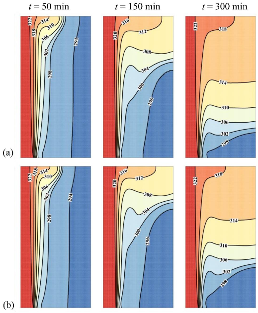
Figure 5 and
Figure 6 depict the isothermal contours and the streamlines in the cavity for two values of the nanoparticle volume fraction, ω
na = 0.06 corresponding to the optimal case and ω
na = 0 corresponding to pure PCM without nanoparticles. The presence of streamlines indicates that the PCM is in the liquid phase; i.e., it has melted in that region. Initially, the PCM starts to melt near the heated tube at the left. In that region, the conductive effects are important. As time goes, the hot melted PCM circulates upwards due to the density difference, and free convection takes place.
A clockwise vortex is created in the domain. The hot PCM impinging in the top region transfers its heat to the melting front so that the convective effects, and consequently PCM melting, are very weak in the bottom part of the cavity compared to its upper part. It can be seen that PCM melting occurs faster in the case ω
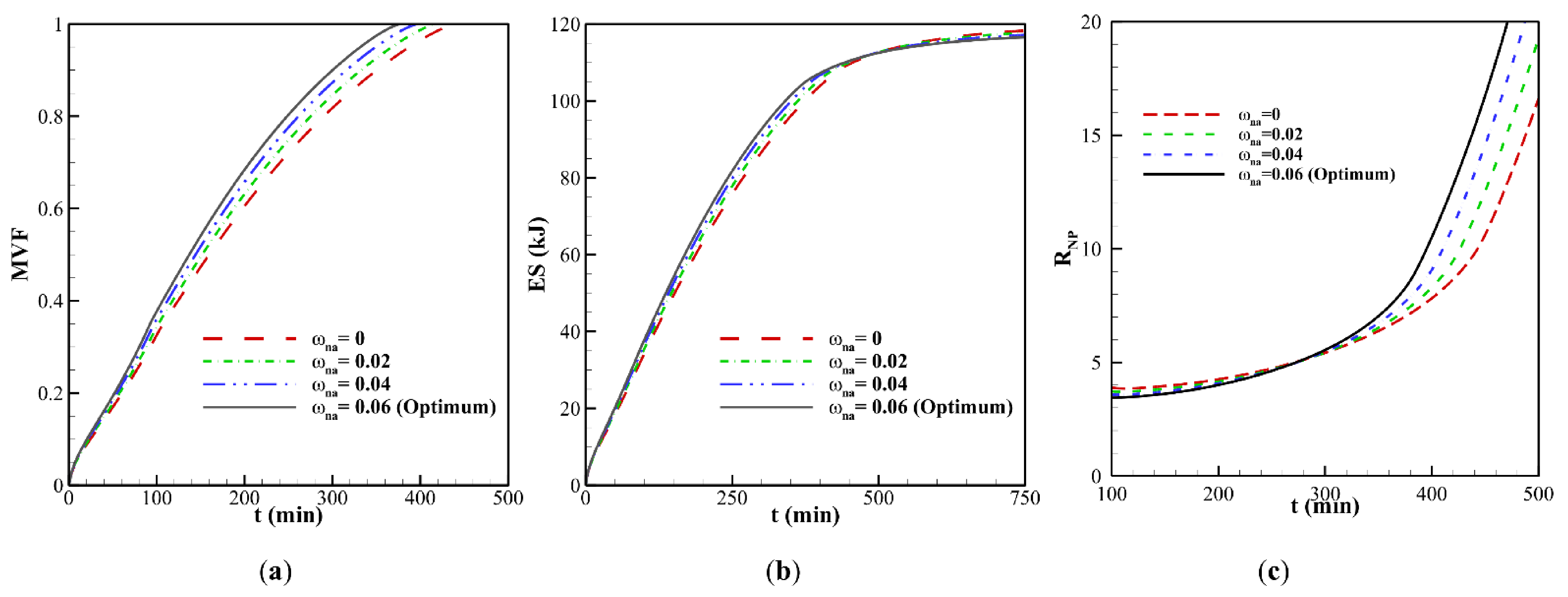
na = 0.06, which is due to conduction heat transfer enhancement at the early stage of melting. It should be noted that the presence of nanoparticles increases the dynamic viscosity of liquid PCM and reduces the strength of natural convection flows at the final stages of melting. This observation is further confirmed in
Figure 7, which illustrates the evaluation of the melted volume fraction MVF and the stored energy ES as functions of time for different values of ω
na. In the charging process, both the MVF and the ES increase for higher values of ω
na. Moreover, full melting (MVF = 1) is achieved faster when ω
na is increased. This is due, as previously explained, to the enhanced thermal conductivity when nanoparticles are added to the PCM, and the growth of dynamic viscosity. The stored energy at 750 min is slightly larger for pure PCM compared to NePCM, which is mainly due to the higher overall latent heat of pure PCM. The presence of nanoparticles reduces PCM’s overall latent heat since they cannot store latent heat. They also slightly increase the heat capacity of the PCM. However, the increase of heat capacity contributing to the sensible heat is much lower than the change in the latent heat. Thus, by using nanoparticles, the ultimate value of stored energy can be reduced slightly.
Figure 7c displays the thermal resistance (
RNP) at the NePCM side for various nanoparticle concentrations. Generally,
RNP increases as the melting advances. By the advancement of melting, the distance of the cold surface (melting front) increases from the heated surface (wavy surface). The increase of distance increases the thermal resistance. This figure shows that at the beginning of melting, where the heat transfer is conduction dominant, the increase of volume fraction of nanoparticles decreases the thermal resistance,
RNP. About 300 min, there is a turning point that the thermal resistance grows as the volume fraction of nanoparticles rises.
Figure 7a shows about 80% melting at 300 min. Thus, at 300 min, a significant amount of liquid PCM exists in the enclosure, and the natural convection heat transfer is significant (see
Figure 6). Therefore, nanoparticle presence increases the dynamic viscosity and reduces the strength of natural convection leading to the growth of thermal resistance.
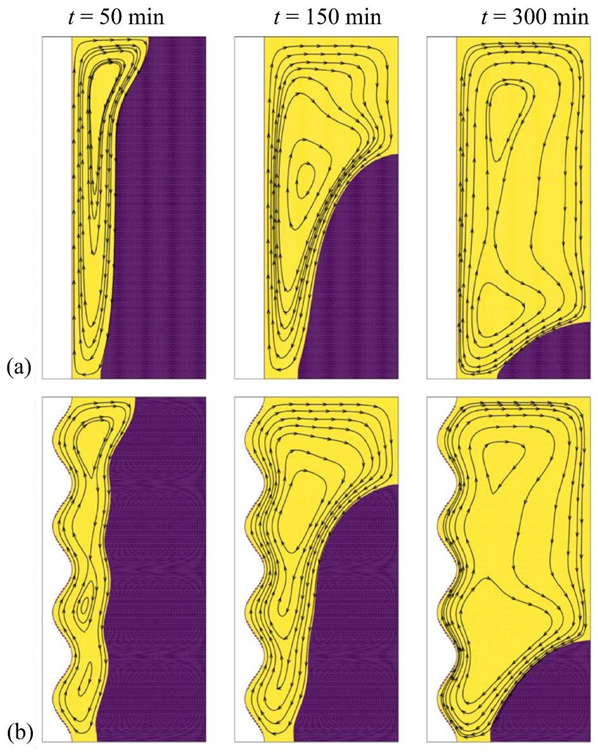
The effect of the hot tube amplitude on the temperature distribution and on the flow-patterns is illustrated in
Figure 8 and
Figure 9. Two amplitudes are considered:
A = 0 (flat tube), which corresponds to the optimal case, and
A = 0.06. It is clear that the streamlines mimic the wavy tube profile in the left portion, where heat is mainly transmitted by conduction. This behavior remains when time passes. However, it is more apparent in the bottom part of the cavity, as convective effects dominate the PCM behavior in the upper part. For Cases 4–6, the steady-state pressure drop was computed as 2.01 × 10
−4 Pa (
A = 1 mm), 6.63 × 10
−3 Pa (
A = 2 mm), and 6.53 10
−2 Pa (
A = 3 mm). The pressure drop of the optimum case is 3.55 × 10
−5 Pa (
A = 0 mm). As seen, there is an exponential pressure drop by the increase of undulation amplitude.
For a fixed N and A, the values of RHTF were changed minimally during the phase change. This is since the HTF fluid-flow is independent of the melting process. The slight changes are from the local variation of the average temperature of the tube during the phase change. The average values of RHTF were found as 0.63 K/W (A = 1 mm), 0.73 K/W (A = 2 mm), 0.65 K/W (A = 3 mm). The RHTF resistance for the optimum design (straight tube) was 0.5 K/W, which is smaller than all wavy cases.
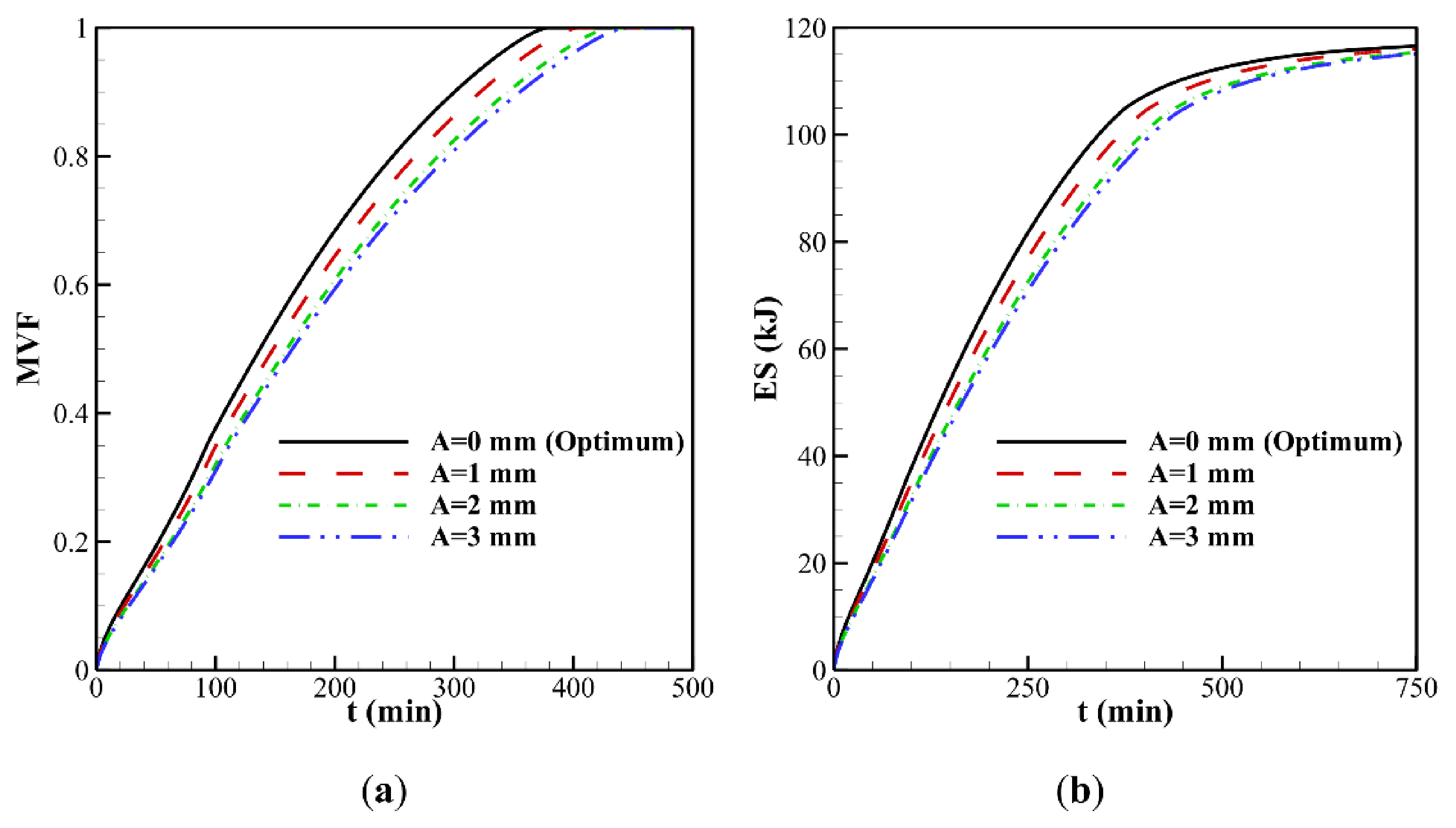
The waviness of the tube increases the distance between the heated line and the PCM and slows down its melting compared to a flat tube. Moreover, the waves act as obstacles that trap the convective flows in the molten region of the enclosure. Thus, the increase of surface contact is not as effective as the suppression of natural convection flow. This appears in the size of the thermal layer near the tube, which is greater for
A = 0. In the upper part of the cavity, this behavior is less effective as the convective effects are dominant. On the other hand, PCM melts faster in the bottom part in the case of a flat-tube. This results in an overall faster PCM melting and a greater volume of liquid PCM for
A = 0. For these reasons, it is clear that reducing
A shows a positive effect on both MVF and ES as indicated in
Figure 10.
The last control factor to be assessed is the number of undulations
N of the wavy tube. The thermal and flow patterns of the PCM in the enclosure are shown in
Figure 11 and
Figure 12 for two values of
N,
N = 4 (the optimal value) and
N = 1, and for the highest wave amplitude of 3 mm. The flow streamlines mimic the wall profile near the hot tube, as the number of oscillations of the streamlines is equal to that of the tube. The volume of melted PCM, as well as the temperature in different zones of the cavity, are larger for
N = 4 compared to
N = 1, which can be attributed to the increase of surface contact between the PCM and the hot tube when the same amplitude is considered. This results in an increase of the MVF and the ES when
N is raised, as observed in
Figure 13. However, the presence of undulation entraps the fluid flow at the tube side and reduces the heat transfer. Thus, on the one hand, the presence of
N contributes to the increase of surface heat transfer, and on the other hand, it reduces the temperature gradients and the intensity of heat transfer.
The analysis of the flow patterns and the isotherms in the enclosure, as well as of the MVF and ES time evolution, confirm the optimization of the design for the determined values of the control factors. For Cases 7–9, the steady state pressure drop was computes as 0.082 Pa (N = 1), 0.080 Pa (N = 2), and 0.072 Pa (N = 3), 3.55 × 10⁻⁵ Pa (the optimum case N = 0). As seen, there is a sharp pressure drop in the presence of undulation compared to the case of a straight tube. The pressure drop reduces as the number of undulations increases. The average values of RHTF were found as 0.64 K/W (N = 1), 0.72 K/W (N = 2), 0.70 K/W (N = 3).


 ,
, 


