Abstract
Nonlinear dimensionality reduction (NLDR) methods such as t-Distributed Stochastic Neighbour Embedding (t-SNE) and Uniform Manifold Approximation and Projection (UMAP) have been widely used for biological data exploration, especially in single-cell analysis. However, the existing methods have drawbacks in preserving data’s geometric and topological structures. A high-dimensional data analysis method, called Panoramic manifold projection (Panoramap), was developed as an enhanced deep learning framework for structure-preserving NLDR. Panoramap enhances deep neural networks by using cross-layer geometry-preserving constraints. The constraints constitute the loss for deep manifold learning and serve as geometric regularizers for NLDR network training. Therefore, Panoramap has better performance in preserving global structures of the original data. Here, we apply Panoramap to single-cell datasets and show that Panoramap excels at delineating the cell type lineage/hierarchy and can reveal rare cell types. Panoramap can facilitate trajectory inference and has the potential to aid in the early diagnosis of tumors. Panoramap gives improved and more biologically plausible visualization and interpretation of single-cell data. Panoramap can be readily used in single-cell research domains and other research fields that involve high dimensional data analysis.
1. Introduction
Recent years have witnessed tremendous interest in single-cell RNA-sequencing (scRNA-seq) or single-cell transcriptomics because scRNAseq makes it possible to investigate transcriptomic variation and regulation at the individual cell level, which may reveal minor but vital changes or cellular heterogeneity that can be easily masked by bulk analysis. The increases in resolution and in big data volume bring about more challenges in data analysis.
While mass cytometry data contain up to 50 parameters or dimensions per single cell [1], a typical scRNAseq analysis task involves a dataset composed of tens of thousands of cells, each expressed as a vector of twenty to thirty thousands of gene expression values or dimensions [2]. However, single-cell data are inherently of much lower dimensionality because many genes may contain zero counts, the genes are not of equal importance and the genes are generally correlated. Therefore, we could develop a dimensionality reduction algorithm to find a low-dimensional representation of biological manifolds on which cellular gene expression profiles lie [3].
The projection from the high-dimensional data space to a low-dimensional one, for downstream tasks such as visualization and data exploration, needs to be conducted in a nonlinear way to reveal the complex structure of the single-cell data [2,3,4,5,6,7]. Manifold learning-based NLDR methods aim to find a lower dimensional representation in which manifold structures are best preserved in terms of some objective criteria.
Numerous manifold learning-based NLDR methods have been used in single-cell data analysis. In particular, t-Distributed Stochastic Neighbor Embedding (t-SNE) [4,5] and Uniform Manifold Approximation and Projection (UMAP) [2,8] are the two most popular ones. UMAP has the ability to better preserve large-scale structures than t-SNE and t-SNE has better performance in visualizing discrete clusters than UMAP [2,7]. Others include locally linear embedding (LLE) [9,10], diffusion map [11], scvis [12], variational autoencoder (VAE) [13,14], scalable deep-learning-based approach (scScope) [15], local tangent space alignment (LTSA) [16,17], isometric mapping (ISOMAP) [17,18,19], GrandPrix [20] and deep count autoencoder network (DCA) [21]. A recent article [22] comparing ten dimensionality reduction methods found that t-SNE and UMAP have the overall best performance. In another study [17], UMAP was found to have good performance for lineage inference analysis.
However, the above leading NLDR methods can suffer from problems in that they may violate the geometrical and topological structures of data [23]. This can result in a low-dimensional embedding that may give misleading information for downstream data exploration tasks.
To address this problem, we applied our recently developed deep learning-based method, called Panoramic manifold projection (Panoramap), by which deep learning of NLDR neural networks is enhanced to have a better ability to preserve the geometrical and topological structures of data. Panoramap achieves this goal by imposing cross-layer structure-preserving constraints [24] on transforms of an encoder neural network to best preserve the structures (Figure 1).
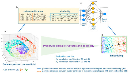
Figure 1.
Schematic overview for Panoramap. The 3-dimensional (high dimensional) Swiss roll residing in 2-dimensional (low dimensional) space is frequently used in machine learning to illustrate the topology-preserving dimensionality reduction algorithm. The rainbow color on the Swiss roll denotes coordinates or positions of the points. A perfect dimension reduction method can unfold the Swiss roll and retain the relationships of the coordinates (preserve the structures). (a) The gene expression data (the blue, green and orange points are shown as illustration) are high dimensional data residing on low dimensional biological manifolds. Each point represents one cell with multiple genes. Cells from one cell type can form a cell cluster (e.g., the blue points form a cluster with high heterogeneity; the green points form a more uniform cluster). (b) The pairwise distances between all the data points (the collection of D1 on (a) are converted to similarity). (c) The similarity matrix is processed in an encoder neural network. (d) The output (two-dimensional embedding) of the Panoramap. We use the correlation coefficient R1 (pairwise distances from all data points) and R2 (from cluster centroids) as evaluation metrics. The pairwise distances between all data points and between cluster centroids on the embedding are well correlated with the original high dimensional space, just as the Swiss roll is unfolded, indicating that the global structures and topology of the original data are preserved. Note that the manifold, the cell data points, the distance lines, etc., are just for illustration purposes, not the real-world depiction. For details of the Panoramap algorithm, please see Section 4.
We evaluated Panoramap across a range of single-cell datasets in comparison with the most popular methods of t-SNE and UMAP. The results demonstrate advantages of Panoramap over both t-SNE and UMAP in several ways: (1) Panoramap reveals the relationships of cell clusters in a better way than t-SNE or UMAP and it is relatively more robust to preprocessing procedures, (2) it excels at demonstrating cell type lineage, (3) it facilitates the discovery of delicate cell types and (4) it helps distinguish premalignant/malignant lesions from other tissues.
2. Results
2.1. Panoramap Preserves Topological and Geometrical Structures of Gene Expression Data
To illustrate the structure preserving property of Panoramap, we used a synthetic dataset (Figure 2a). The original two-dimensional image inspired from reference [25] consists of seven clusters of clouds, spirals and circles plus grey-colored scatter noises and bridge-like noises. The two-dimensional coordinates were mapped to a 20-dimensional space by linear, trigonometric, exponential and logarithmic transformations (see Section 4) inspired by reference [6]. Then, the 20-dimensional data were used as inputs to t-SNE, UMAP and Panoramap, respectively. The results demonstrate that Panoramap keeps the topological and geometrical structures of the clusters better than t-SNE and UMAP. The circles and spirals remain intact in Panoramap, while they are broken or form artificial structures in t-SNE and UMAP. The relative spatial positions of clusters in Panoramap are most similar to those on the original image, indicating the inter-cluster distances are preserved best in Panoramap. Additionally, the grey-colored scattered noises are visible in Panoramap while they are hidden in other bigger clusters in t-SNE and UMAP embeddings. Panoramap also has some limitations. The bridge-like noise dots are “broken” in Panoramap as they are in t-SNE and UMAP.
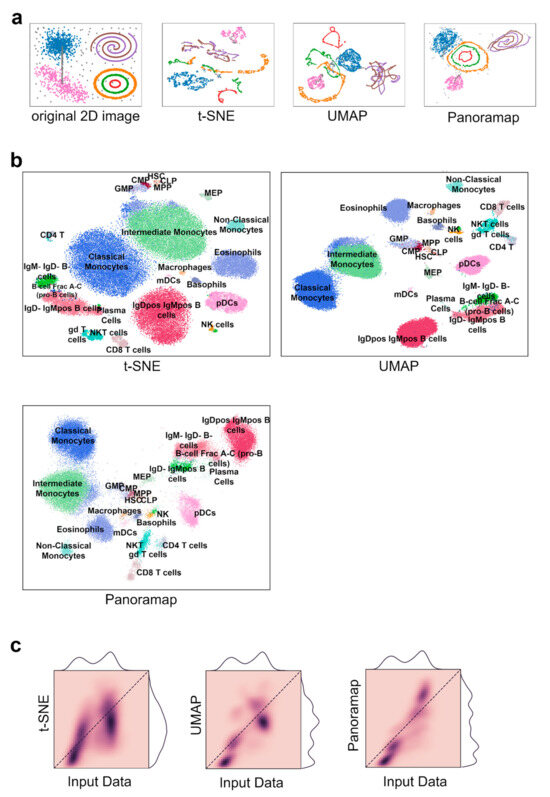
Figure 2.
Panoramap best preserves topological and geometrical structures of input data. (a) A mixture of 7 distinct manifolds and ambient noise (grey color) in 2-dimensional (2D) are transformed to 20-dimensional space nonlinearly and then used as the inputs to Panoramap, t-SNE and UMAP. From left to right shows the original image and the resulting embeddings. Topological structures are violated in the t-SNE and UMAP embeddings but preserved in the Panoramap embedding. (b) Embeddings from t-SNE, UMAP and Panoramap on the Samusik01 dataset, colored by cell type. HSC, hematopoietic stem cells; MPP, multipotent progenitors; CLP, common lymphoid progenitors; CMP, common myeloid progenitors; GMP, granulocyte-myeloid progenitors; MEP, myeloid-erythroid progenitors; pDCs, plasmacytoid dendritic cells; mDCs, myeloid dendritic cells; gd T cells, γδ T cells; NK cells, natural killer cells; NKT cells, natural killer T cells. (c) Two-dimensional histograms representing correlation between pairwise distances in high dimensional input space and 2D embedding space for the Samusik01 dataset. Pairwise distances in Euclidean distances in 50 bins from both the high dimensional space and the embedding space are plotted and colored according to the normalized density of the binned distances. A perfect correlation is that all dark points are on the diagonal and that the distance distribution curves on the top (for input data) and on the right (for embedding space) are identical.
The structure-preserving properties of Panoramap displayed on the synthetic dataset can have positive implications in single-cell data analysis. The topology of gene expression patterns has been used to study continuous cell developmental trajectory and transcriptional repertoires [26]. Topology studies the relationships of nearness or proximity qualitatively without using distances, whereas geometrical structure can be studied with quantitative distance metric functions [27]. Therefore, the geometry of gene expression has been studied to characterize the similarity and diversity of the cells and classify biological phenotypes [28]. Previous studies have shown that unsupervised dimensionality reduction could suggest the relevant landmark genes to establish a preliminary input spatial map and that gene expression patterns from scRNAseq can be inferred to spatial geometric structures [29].
Because Panoramap better preserves the topological structures (e.g., Panoramap preserves intact circles in Figure 2a) and the geometrical structures (e.g., Panoramap preserves global structures and retains the spatial positions of clusters in Figure 2a) in the synthetic dataset, it is plausible that Panoramap can better reveal the relationships of cell clusters, which is the basis to determine the hierarchy of cells or to depict the continuous cell states. Because Panoramap discloses noise points in the synthetic dataset which are concealed in bigger clusters in t-SNE or UMAP (Figure 2a), it is feasible that Panoramap can uncover rare cell types.
We used mass cytometry dataset and scRNAseq datasets to verify our hypothesis. The single cells used for comparison in this study are from various tissues and from both human and mouse (Supplementary Table S1). The cell numbers range from thousands to tens of thousands. The packages of t-SNE and UMAP integrated in the Scanpy [30] toolkit were used for comparison. For all the compared NLDR methods, we used as the input data 50 principal components (PCs) for the scRNAseq datasets and all the original 38 dimensions for the mass cytometry dataset, which is consistent with the default settings of t-SNE and UMAP in Scanpy.
The Samusik01 dataset [1] reflects murine bone marrow hematopoiesis. As is shown in Figure 2b, the embedding from Panoramap is quite similar to that of UMAP with hematopoietic stem cells (HSCs) in the center and mature cells in the peripheral. Myeloid cells are grouped on one side and lymphoid cells are arranged on the other side. The two subgroups of CD8 T cells which are divided by CD44 and Ly6C (a marker of central memory cells [1,31]) are more distinct in Panoramap, as are the subgroups of plasmacytoid dendritic cells (pDCs) (Figure S1). Cell clusters on t-SNE embedding seem not follow the clear pattern that cells of the same origin are grouped together. The phenomenon is consistent with the features of the algorithms, with UMAP and Panoramap preserving global structures better than t-SNE. To quantify the global structure preservation of embeddings, we performed 2D histogram using the methods from reference [32], which show that Panoramap has the best correlation of unique cell–cell distances between the high-dimensional space and embedding space (Figure 2c).
To further assess quantitively the preservation of global structures, we used the following metrics:
R1: Pearson correlation coefficient between pairwise distances of all sample points in the high-dimensional space and in the embedding.
R2: Pearson correlation coefficient between pairwise distances of cluster centers in the high-dimensional space and in the embedding.
R = (R1 + R2)/2: The averaged value providing an overall performance metric for the evaluation of structure preservation quality.
Table 1 shows the metrics from one experiment for all the datasets. Panoramap generally has the best performance in preserving global structures and inter-cluster relationships. With repeated experiments, the trend remains the same and the performance of Panoramap is stable (Figures S2 and S3).

Table 1.
Overview of evaluation metrics on the four datasets used in this study.
2.2. Panoramap Is More Robust to Preprocessing Methods
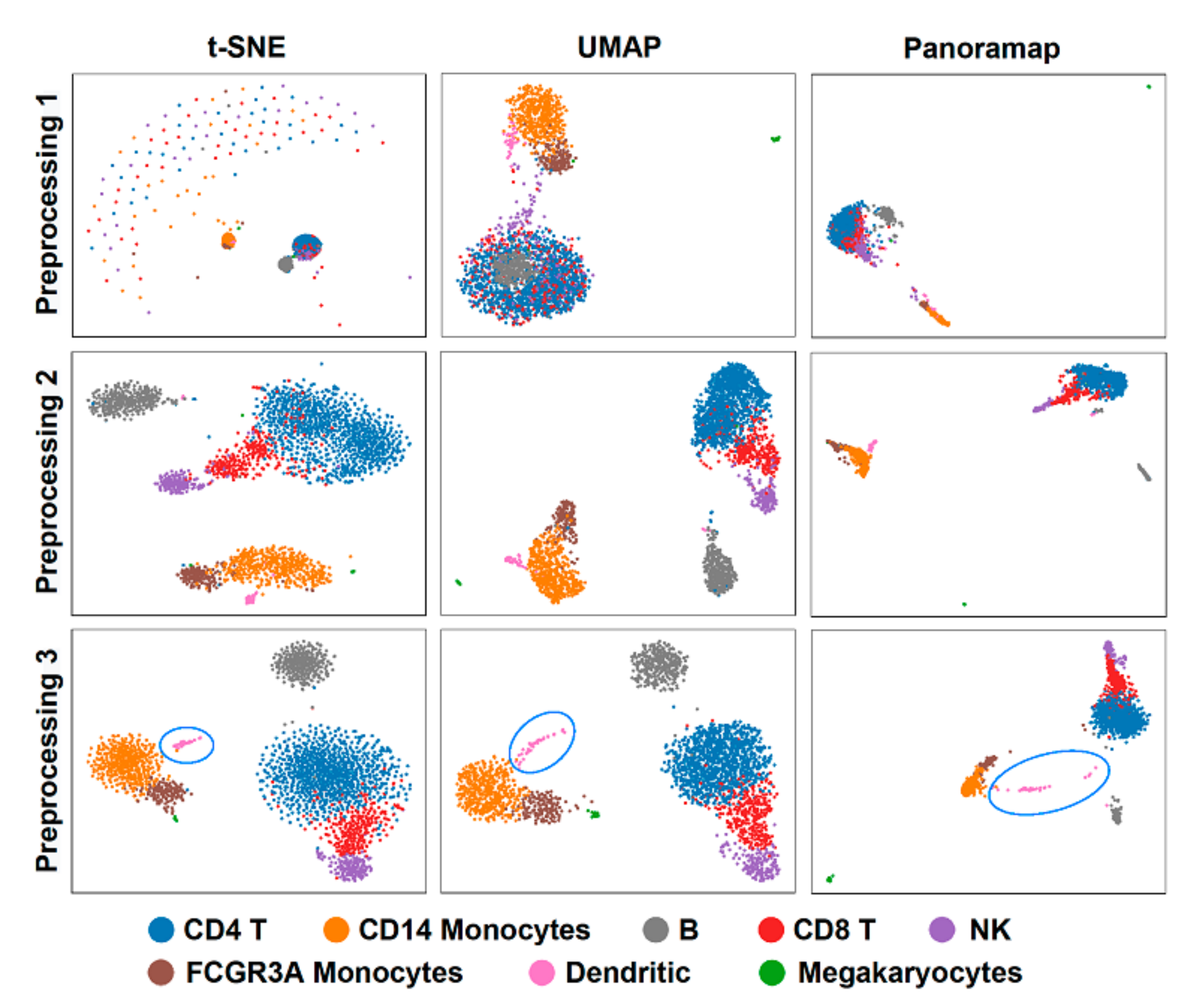
Data preprocessing is necessary in data analysis and sometimes different preprocessing methods can lead to contradictory results. To investigate the effect of preprocessing methods on embeddings, we compared the embeddings using dataset PBMC3k (peripheral blood from a healthy donor, downloaded from 10x website) [33] under three preprocessing procedures: (1) normalization + logarithm, (2) normalization + logarithm + Principal Component Analysis (PCA) and (3) normalization + logarithm + selection of highly variable genes + scale + PCA (standard pipeline in Scanpy [30] PBMC tutorial [34]). Then, we performed the clustering using Leiden [35] and cell type annotation according to the Scanpy tutorial. The results show that Panoramap is relatively more robust under different preprocessing procedures (Figure 3), while t-SNE and UMAP embeddings change more significantly; for example, t-SNE has crescent-like points and UMAP has B cell points inside the T cell points in the first preprocessing condition (Figure 3). The evaluation metrics R1, R2 and R with different preprocessing methods on the PBMC3k dataset (Table 2) also confirm that Panoramap best preserves intrinsic properties of the original high dimensional data in all the preprocessing conditions.
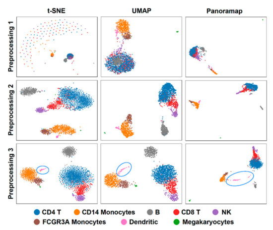
Figure 3.
Panoramap is stable and robust to preprocessing methods. t-SNE and UMAP may have artefacts or violate topological structures. Preprocessing 1: normalization + logarithm. Preprocessing 2: normalization + logarithm + PCA. Preprocessing 3: normalization + logarithm + selection of highly variable genes + scale + PCA. The blue circles highlight the dendritic cells in Preprocessing 3.
Table 2.
Effect of different preprocessing methods on the evaluation metrics for the PBMC3k dataset.
2.3. Panoramap Embedding Better Reveals Cell Lineage or Cell Hierarchy Quantification
For the PBMC3k dataset in Figure 3, there is a remarkable discrepancy between Panoramap embeddings and those of t-SNE and UMAP that relies on the position of megakaryocytes. Preprocessing 3 in Figure 3 is the standard preprocessing procedure in Scanpy or Seurat, and we analyze the embeddings under this condition in the following text. Panoramap separates PBMCs into three distinct groups: (1) megakaryocytes; (2) myeloid cells including monocytes and DC; and (3) lymphoid cells including T cells, B cells and NK cells, which is consistent with cell lineage. To explore the relationships between cell clusters in the original high dimensional space (refers to the native gene expression data space after normalization and logarithm preprocessing) and the embedding space, we made hierarchical dendrograms based on gene expression distances between cell clusters in both the high dimensional space and the embedding space. We found that the dendrogram derived from the high dimensional space is most in line with the blood cell lineage. Moreover, among the compared NLDR methods, the dendrogram from Panoramap embedding is closest to that from the high dimensional space, with the cluster of megakaryocytes deviating from other clusters in the dendrograms (Figure 4). By quantified comparison of hierarchical clusters using the element-centric clustering comparison method from reference [36], the dendrogram from Panoramap embedding is shown to rank the highest among the NLDR methods in terms of a similarity score [36] S (see Section 4).
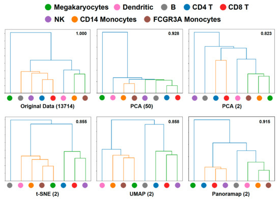
Figure 4.
Dendrogram confirms that Panoramap embedding is in accordance with cell lineage or hierarchy. Dendrograms from PBMC3k dataset in the original 13714-dimensional high dimensional space, the 50-dimensional PCA spaces, 2-dimensional PCA space, t-SNE, UMAP and Panoramap embedding spaces using Euclidean distances. The numbers on the upper right corner of each dendrogram denote similarity scores [36] compared with that from original space. Similarity score is between 0 and 1. High similarity score indicates more similarity between compared dendrograms.
2.4. Panoramap Better Reveals Delicate Cell Populations
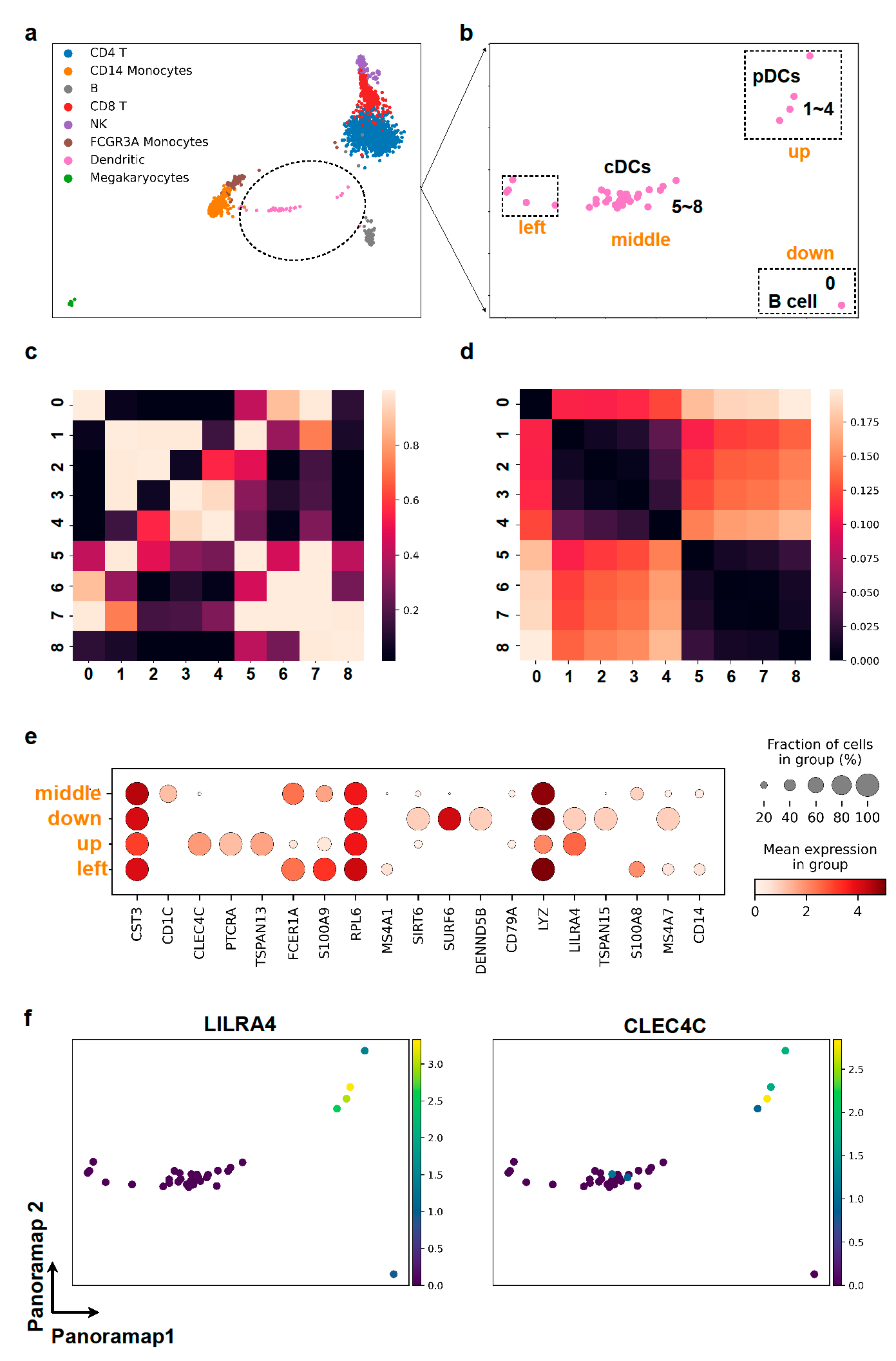
In the Panoramap embedding for the PBMC3k dataset, there appear some “out-of-distribution” data points, such as those between T cells and B cells that are colored by dendritic cells (DCs) (Figure 3 Preprocessing 3, Figure 5a,b). However, there are no such “out-of-distribution” points in t-SNE and UMAP (Figure 3 Preprocessing 3), because such points of small data size are attracted to the main dendritic cell cluster in the t-SNE and UMAP, as in the case of hidden noise points with the synthetic dataset shown in Figure 2a.
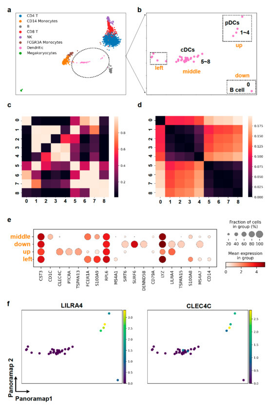
Figure 5.
Panoramap reveals delicate cell populations. (a,b) In Panoramap embedding for PBMC3k dataset, the dendritic cell population is separated into one major group in the middle (e.g., points 5–8) and several points (points 1–4) up between B cells and T cells, one point down which is very close to B cells (point 0) and several points on the left near the monocytes. (c) Heatmap from pairwise distance derived similarity in high dimensional space shows that points 1–4 are close to each other and points 5–8 are close to each other. Brighter color denotes more similarity or more proximity. (d) Heatmap from pairwise Euclidean distances in Panoramap embedding space shows that points 1–4 are close to each other and points 5–8 are close to each other. Darker color denotes less distance or more proximity. (e) Dot plot for selected gene expressions from the 4 subclusters in dendritic cell population. The color represents the mean expression within each of the subclusters and the dot size indicates the percentage of cells in the subcluster expressing a gene. (f) Scatter plots for gene expressions of LILRA4 and CLEC4C (pDC markers) in dendritic cell cluster. Yellow color represents high gene expression and dark blue denotes low gene expression.
To elucidate whether these points are meaningful in Panoramap embedding, we scrutinized the points closely. We subset the dendritic cells and conducted more analysis. From the differentially expressed genes, we found out that the points between B cells and T cells are plasmacytoid dendritic cells (pDCs) with high expression of CLEC4C, PTCRA, TSPAN13, LILRA4, etc. (Figure 5e,f). The pDCs are differentiated independently of the myeloid conventional DC (cDCs) lineage. They derive from common lymphoid progenitors and are close to lymphoid cells in lineage [37]. We also calculated the distance derived similarity in high dimensional space and the pairwise distances in Panoramap embedding for selected dendritic cells for quantification. The heatmap of similarity shows that the out-of-place points are indeed far from other dendritic cells in high dimensional space (Figure 5c), and that the proximity of data points in embedding (Figure 5d) corresponds well with the similarity of data points in high dimensional space (Figure 5c). Therefore, the Panoramap embedding best reflects the intrinsic property of original data and the distances between data points in Panoramap embedding are related to the discrepancy of cell types, enabling the discovery of delicate cell populations.
2.5. Panoramap better Displays Cell Types in Accordance with Cell Development
Trajectory inference can be used to simulate the cell development. However, the pseudotime estimated by algorithms is not always reliable and experimental data of “ground truth” are lacking [38]. Figure 6 shows cell trajectory analysis on the dataset from murine adipose tissue from reference [39]. Unsupervised Louvain [40] clustering was performed on the latent layer and cell types were determined according to markers from reference [39]. Apart from the cluster size in Panoramap being a bit smaller, there are several differences between Panoramap and UMAP embeddings. For example, the adipocyte (blue) cluster in UMAP is between two clusters of committed Icam1+ preadipocytes (Figure 6a). In Panoramap the pink Icam1+ preadipocyte clusters with more G2M cells reside closely to the brown Icam1+ preadipocyte cluster, and the blue adipocyte cluster is in clear distinction to preadipocytes (Figure 6d). Similarly, the purple cluster which is an interstitial progenitor with more G2M cells and is in proximity with the pink Icam1+ preadipocyte cluster in UMAP is close to the red interstitial progenitor cluster. Thus, Panoramap embedding provides more meaningful relationships among clusters and resembles that of UMAP with Partition-based graph abstraction (PAGA) [41] initialization (Figure 6c), indicating that the arrangement of clusters on Panoramap embedding is consistent with cell development. While using UMAP, one needs to perform PAGA for trajectory inference and then may visualize embedding using PAGA initialization; Panoramap can achieve a similar function with much simpler steps.
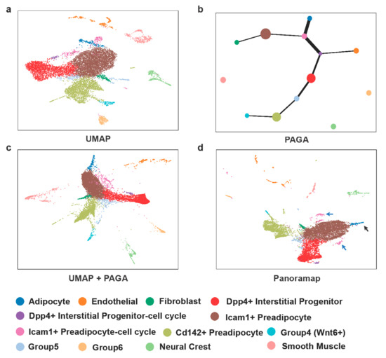
Figure 6.
Cell types displayed with Panoramap correlate well with cell development. (a) UMAP embedding of cells from murine adipose tissue. (b) Trajectory inference using PAGA. (c) UMAP with PAGA initialization. (d) Panoramap embedding for the murine adipose tissue. The black arrow points to adipocytes and the blue arrow points to the interstitial progenitors with more G2M cells.
2.6. Panoramap better Distinguishes Premalignant/Malignant Lesions from other Tissues
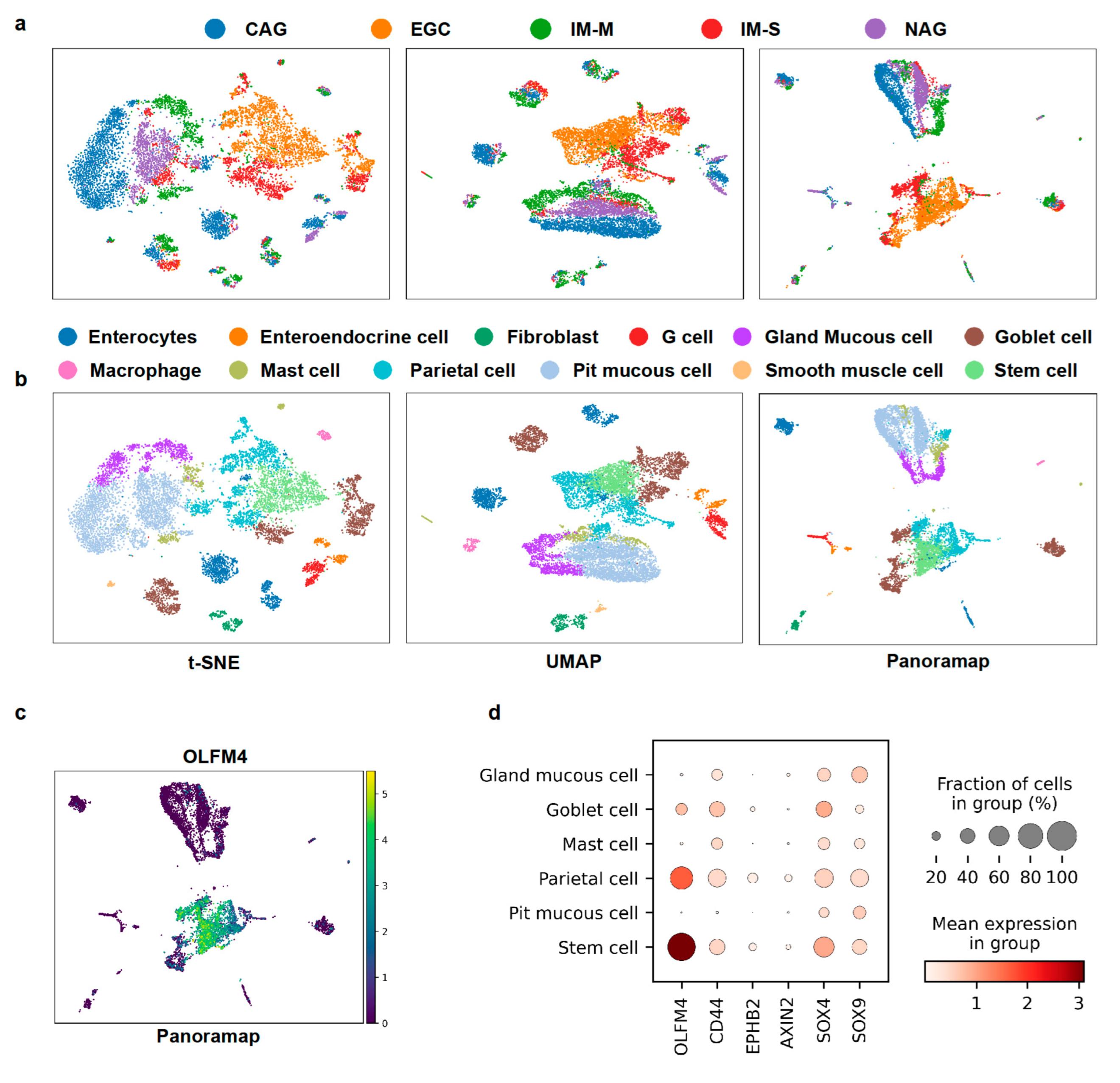
Because Panoramap can reveal cell lineage or hierarchy and unveil rare cell types, we wondered whether Panoramap can facilitate early tumor detection. Atrophic gastritis and intestinal metaplasia are premalignant conditions which can lead to gastric cancer. The annual incidence of gastric cancer is 0.1% for patients with atrophic gastritis, and 0.25% for intestinal metaplasia [42]. Among intestinal metaplasia (IM), the severe type of intestinal metaplasia is a significant risk factor for gastric cancer, because the age-adjusted early gastric cancer rate per 100,000 person-years with severe intestinal metaplasia is more than 5-fold that with moderate intestinal metaplasia and more than 20-fold that with mild intestinal metaplasia. Moreover, patients with severe intestinal metaplasia have shorter time intervals between the time at baseline endoscopy and the onset of subsequent early gastric cancer [43]. The gastric cancer dataset from references [44,45] contains cells from patients with early gastric cancer (EGC), intestinal metaplasia with severe level (IM-S), chronic atrophic gastritis (CAG), non-atrophic gastritis (NAG) and intestinal metaplasia with mild level (IM-M). After preprocessing, the dataset contained 10638 cells and 1457 genes. We used the default settings for Louvain [40] clustering and annotated cell types using the marker genes from reference [44]. In Panoramap and UMAP embeddings there are two distinct groups: (1) the early gastric cancer and severe intestinal metaplasia and (2) the CAG, NAG and IM-M (Figure 7a). Gastric cancer is usually surrounded by severe intestinal metaplasia in pathological images in the real world and patients with severe intestinal metaplasia have the greatest risk for developing gastric cancer. The two distinct groups are more predominant in Panoramap embedding. Another discrepancy between Panoramap and UMAP or t-SNE embeddings is that in UMAP the mild intestinal metaplasia cluster is closest to the gastric cancer/severe intestinal metaplasia group. In Panoramap the CAG, NAG and IM-M seem to have similar distance with the gastric cancer/severe intestinal metaplasia group, with the gland mucous cell cluster closest to the gastric cancer/severe intestinal metaplasia group. The gastric mucous cells are composed of pit mucous cells and gland mucous cells (GMCs) with different gene expression patterns. The intestinal stem cell marker OLFM4 is mainly expressed in GMCs compared with pit mucous cells [44]. The expression of OLFM4 increases from CAG to IM to early gastric cancer. OLFM4-expressing GMCs were rarely detected in the CAG lesion (0.4%), while their number remarkably increased in the mild IM lesion (8%) and reached a peak in the severe IM lesion (26%) [44]. The proportion of OLFM4-expressing cells reached the peak in the early gastric cancer lesion, although GMCs disappeared in the early gastric cancer lesion [44]. This suggest that GMCs that tend to acquire the intestinal-like stem cell phenotype might be the crucial cellular characteristics for gastric IM and gastric tumorigenesis [44]. Moreover, the close relationship between GMCs and the gastric cancer/severe intestinal metaplasia group is echoed in Panoramap embedding with the increasing intestinal stem cell gene expressions from pit mucous cells to GMCs to parietal cells and stem cells (Figure 7b–d), suggesting that Panoramap embedding is more consistent with the development of cancer and has the potential to aid in early tumor detection.
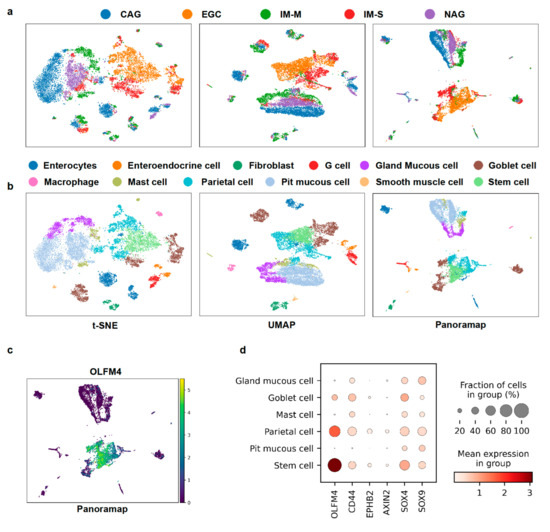
Figure 7.
Panoramap helps distinguish premalignant/malignant lesions from other tissues. (a) For the gastric cancer dataset, embeddings from t-SNE, UMAP and Panoramap are colored according to the histological diagnosis provided in reference [44]. In Panoramap embedding, early gastric cancer lesion (EGC, orange color) and intestinal metaplasia (IM-S, red color) lesion of severe level are clearly separated from CAG, NAG and IM-M. (b) For the gastric cancer dataset, embeddings from t-SNE, UMAP and Panoramap are colored by cell types. (c) Scatter plot of gene expression for OLFM4. (d) Dot plot for intestinal stem cell gene expressions. The color represents the mean expression within each of the cell clusters and the dot size indicates the percentage of cells in the cluster expressing a gene. CAG, chronic atrophic gastritis; NAG, non atrophic gastritis; IM-M, intestinal metaplasia with mild level.
3. Discussion
In this work, we applied Panoramap for dimensionality reduction and visualization for single-cell data analysis and demonstrated advantages of Panoramap over t-SNE and UMAP. Panoramap better preserves topological and global geometrical structures during NLDR. Therefore, Panoramap can be used when t-SNE and UMAP fail to reveal rare cell types or hierarchical relationships. Panoramap can facilitate cell development trajectory inference, rare cell type discovery, and has the potential to distinguish tumor cells from normal cells.
In single-cell data analysis, the gene expression count data during preprocessing are usually normalized to make them comparable between cells. After normalization, data matrices are typically log(x+1) transformed. The log transformation reduces the skewness of the data to approximate the assumption of many downstream analysis tools, including Panoramap, that the data are normally distributed [3]. Panoramap gives preliminary results in line with blood cell lineage after normalization and logarithmic transformation as shown in Preprocessing 1 in Figure 3, while t-SNE and UMAP need more preprocessing steps. Panoramap could handle input data with distributions other than normal distribution when the appropriate is assigned in the input layer. More work needs to be done in the future to explore the relationship between the distribution of the input data and the optimization of Panoramap.
The Panoramap embedding reveals more meaningful structures than the compared methods. For example, the cDCs and pDCs clusters can be separated clearly in Panoramap as in Figure 5. Similarly, the CD8 T cells are subdivided into two groups in Panoramap (Figure 2b) with central memory CD8 T cells (CD44+Ly6C+) in one group and CD44-Ly6C- cells in another (Figure S1). Thus, another future direction would be to explore the possibility to combine dimensionality reduction and clustering together so that the processing pipeline for single-cell data analysis can be further refined and the time for data analysis can be shortened.
Finally, the embeddings of Panoramap demonstrate consistency with cell type lineage or hierarchy. It would be interesting to investigate whether this phenomenon can help identify novel genetic biomarkers or gene expression patterns linked with certain phenotypes.
We hope that with the merit of well preserving global structures and delineating cell type lineage or hierarchy, Panoramap can help make new discoveries in single-cell research for cancer diagnosis, cell lineage determination, cell development and other research fields.
4. Materials and Methods
4.1. Panoramic Manifold Projection (Panoramap) and Geometry-Preserving Loss
Panoramap is a deep learning neural network framework enhanced by geometry-preserving constraints [23,24]. The major differences between t-SNE/UMAP and Panoramap are that Panoramap is a learnable and reusable neural network transformation, and Panoramap uses a different definition of similarity. Different from t-SNE/UMAP, which compute similarity in data space and embedding space using distinct formulae, we unified the definition of similarity in data space and embedding space. We also introduced a hyperparameter , the continuous change of which modulates the balance between attractive forces and repulsive forces, resulting in a better preservation of global structures while keeping a similar performance of preservation of local structures. For details, please refer to [23,24].
In short, Panoramap is an abridged form of autoencoder, which by itself is suitable for dimensionality reduction, but without the reconstruction part. Panoramap is composed of an input layer, several dense layers of neurons and an output layer.
The geometry-preserving loss function is used in Panoramap to train the network, which is originated from the cost function of LargeVis and UMAP, the cross entropy [8]:
where and are the undirectional similarities between point and point at the input layer and the output layer , respectively. We simplified the cost function by removing the and the on top of the fractions because they are fixed values given a dataset. The undirectional similarities are defined as follows [2,4,23]:
where is a directional similarity based on a normalized squared t-distribution, which converted from the Euclidean distance between point and point [4,23] is
where is the degrees of freedom in the t-distribution, and
is the normalizing function of which sets the limit .
The is used to calibrate locally about at the input layer, where is the nearest neighbor set. The scaling parameter is estimated from the data by best fitting to the following equation [2,4,23]:
where is a given perplexity-like hyper-parameter. In the input layer, we assume that the input layer data distance satisfies a normal distribution and use a t-distribution with to approximate it. will be determined by binary search, and, from algorithmic efficiency considerations, we set . In the original paper of reference [23], a threshold for distance standard deviation was defined to force individual to be identical by averaging all data points.
Panoramap takes a random initialization which is different from t-SNE, UMAP, etc. whose performances are highly dependent on their initialization [46] (Figure S4).
Panoramap is based on manifold learning and manifold assumption. Manifolds are locally Euclidean; thus, Euclidean distance is used. We also tested the algorithm with other distance metrics, such as the geodesic distance, and the performance was similar (Table S2). More discussions about the choice of metrics or other versions of the algorithm are beyond the scope of this manuscript.
The training time for Panoramap is dependent on the number of epochs and samples. The time consumed for training Panoramap is comparable to other neural network algo-rithm [47]. As for test run time, Panoramap is the shortest, even shorter than t-SNE and UMAP (Figure S5).
4.2. Visualization
Similar to t-SNE and UMAP, the Panoramap module can be integrated in Scanpy [30] (https://github.com/theislab/Scanpy, accessed on 1 November 2020) for dimensionality reduction and visualization. The default settings in Scanpy were used for t-SNE, UMAP and PCA unless specified in the text. For Panoramap, we used default settings (perplexity = 50, batch size = 2000, learning rate = 0.001. We used two types of network structures: network structure [500,500,2] and epoch 1700 for mass cytometry data (Samusik01 dataset); network structure [500,300,100,2] and epoch 1200 for scRNAseq datasets (PBMC3k, Adipose_tissue, Gastric_cancer datasets). Although it is possible to optimize the hyper-parameters for best performance, we used the fixed default settings for fair comparison with t-SNE and UMAP in this article. For scatter plots, dot plots and PAGA, we used the integrated methods in Scanpy.
The heatmap in Figure 5 was plotted using the Seaborn package in Python using pairwise distances in embedding space or pairwise similarities in high dimensional space (after normalization and logarithm, with 13,714 dimensions).
4.3. Data Preprocessing
We used 3 preprocessing methods in Figure 3 to test the robustness of Panoramap, t-SNE and UMAP. Preprocessing was done using Scanpy [30]. The tutorial of Scanpy for preprocessing can be found in Preprocessing and clustering 3k PBMCs—Scanpy documentation (https://scanpy-tutorials.readthedocs.io/en/latest/pbmc3k.html, accessed on 1 November 2020). In short, for Preprocessing 1 (normalization + logarithm) in Figure 3, the gene expression matrix is used to construct the AnnData object. Then, basic filtering is conducted to filter out genes that are detected in less than 3 cells and to filter out cells that contain less than 200 genes. After that, cells that have more than 5% counts in mitochondrial genes are removed. Then, the total count of the data matrix is normalized to 10,000 reads per cell, so that counts become comparable among cells, and the data are logarithmized. The data matrix contains 13714 genes after normalization and logarithm. The matrix data are used as inputs to NLDR. The “.raw” attribute of the AnnData object is set to the normalized and logarithmized raw gene expression for later use, e.g., the high dimensional data for calculating the correlation coefficient or dendrogram or heatmap are the raw matrix data after normalization and logarithm.
For Preprocessing 2 (normalization + logarithm + PCA), after Preprocessing 1, we reduce the dimensionality of the matrix data by running principal component analysis (PCA). The first 50 principal components are then used as inputs to NLDR.
For Preprocessing 3 (normalization + logarithm + selection of highly variable genes + scale + PCA), after Preprocessing 1, highly variable genes are identified and selected. The matrix is sliced to filter out genes that are not highly variable. Then, the effects of total counts per cell and the percentage of mitochondrial genes expressed are regressed out. The data are scaled to unit variance. Values exceeding standard deviation 10 are clipped. Then, the dimensionality of the data is reduced by running PCA. The first 50 PCs are used as inputs to NLDR. This Preprocessing 3 is the standard preprocessing in Scanpy and is mostly used in this manuscript unless otherwise stated.
4.4. Datasets
Synthetic dataset: The synthetic dataset was inspired by reference [25] and https://github.com/deric/clustering-benchmark, accessed on 1 November 2020. The two-dimensional coordinates were mapped to a 20-dimensional space by the transformation , , , , , , , , , , , , , , , , , , , inspired by reference [6]. Then, the 20-dimensional data, after fit transform using StandardScaler in sklearn, were used as the input to Panoramap, t-SNE and UMAP, respectively.
For Panoramap, we used a perplexity of 50, -start of 0.01, trace from 0.01 to 0.5 from epoch 400 to 800, and a network structure [200,2] with a batch size of 1000. For t-SNE and UMAP, default settings in Scanpy were used.
PBMC3k dataset: The PBMC3k dataset was downloaded from 10x company (https://support.10xgenomics.com/single-cell-gene-expression/datasets/1.1.0/pbmc3k, accessed on 1 November 2020). Preprocessing followed the procedure in Preprocessing and clustering 3k PBMCs—Scanpy documentation (https://scanpy-tutorials.readthedocs.io/en/latest/pbmc3k.html, accessed on 1 November 2020). After preprocessing, 2638 cells x 1838 highly variable genes were used for dimension reduction and visualization.
Samusik01 dataset: We used the Samusik01 dataset matrix and annotation from reference [1,2]. This dataset is from mouse bone marrow cells. An arcsinh transformation with a cofactor of 1 was used [2]. Ungated cells were removed before analysis and we obtained 53,173 cells × 38 genes for dimension reduction.
Adipose_tissue dataset: We used the murine adipose tissue dataset, with the GSM3717977_SCmurinep12 data from GSE128889_RAW data [39]. After preprocessing using the methods from reference [39], we obtained 11420 cells × 1415 highly variable genes.
Gastric_cancer dataset: We used the data with GSE 134,520 from reference [44,45]. We used all the cells from sample CAG1, EGC, IMS3, IMW1 and NAG3 to cover all the histological types and to reduce data size. After preprocessing using the methods from reference [44], we obtained 10,638 cells × 1457 highly variable genes.
A summary of single-cell datasets can be found in Supplementary Table S1. Processed datasets in h5ad form can be found at https://doi.org/10.6084/m9.figshare.20010545.v1, accessed on 1 November 2020.
4.5. Evaluation Metrics
Two-dimensional histogram: Heiser et al. presented a quantitative framework for evaluating single-cell data structure preservation [32] and we used the 2D histogram to compare the preservation of global structure of Panoramap, t-SNE and UMAP on the Samusik01 dataset. Pairwise cell–cell distances in the native gene space and embedding space were calculated. Then, a 2D histogram was built using correlated binned distances from the native space and embedding space. For details, please refer to reference [32].
R1: The gene expression matrix is represented as an (cells/rows/observations) × (genes/columns/features) matrix. A pairwise distance (between cells) matrix was calculated for high dimensional space (using the raw data after normalization and logarithm) and for embedding space, respectively, using Euclidean_distances in sklearn. Then, the upper triangular part of the symmetric matrix excluding the diagonal 0 was used to calculate the Pearson R between high dimensional space and embedding space.
The formulae are as follows:
where is the Pearson correlation function, is the Euclidean distance, is the observation/cell, is the number of the observations/cells, denotes high dimensional space and represents embedding space.
R2: The gene expression matrix is represented as an (cells/rows/observations) × (genes/columns/features) matrix. The centroid of each cell cluster was calculated using the average of gene expression values across columns, so that each centroid was a vector of elements ( equals to dimensions of the raw data after normalization and logarithm for high dimensional space, or equals to two for embedding space). Pairwise distances between the centroids were calculated using Euclidean_distances in sklearn. Then, the Pearson R of distances between high dimensional space and embedding space was calculated using the upper triangular part excluding the diagonal.
The formulae are as follows:
where is the centroid (mean of the data across columns/features/genes) of cluster in high dimensional space and represents the centroid (mean of the data across columns/features/genes) of cluster in embedding space. is the number of clusters.
R: This is an overall performance metric calculated as R = (R1 + R2)/2.
For scRNAseq datasets, the high-dimensional data used in this article unless specified otherwise in the text were after preprocessing by normalization and logarithm (which are the raw data or adata.raw in AnnData using Scanpy). These data have not undergone the process of selecting for highly variable genes, scaling or principal component analysis (PCA). The advantage is that these native data are not influenced by preprocessing methods or analysis toolkits, leading to a more fair comparison among different methods.
We tested using geodesic distances in high dimensional space and Euclidean distances in embedding to calculate R1 (Supplementary Table S2) and found that the results were quite similar to those with Euclidean distances in both high dimensional space and embedding space. Thus, we used Euclidean distance in high dimensional space in this manuscript to simplify the calculations.
S: Similarity score [36] denotes the similarity between compared dendrograms, ranging from 0 and 1. A high similarity score indicates more similarity between compared dendrograms. Please see Section 4.6 and similarity score for details.
The formula is as follows (see reference [36]):
where is the average of the element-wise similarities between and dendrograms and is the number of clusters. Element here denotes cluster centroid. For detailed formulae, please see reference [36].
4.6. Dendrogram
In the PBMC3k dataset, we used Euclidean distances in both high dimensional space and embedding space between clusters to construct dendrograms. For the original high dimensional space, we used the raw data space after normalization and logarithm which is the same as calculating R1 and R2. For all the spaces, we calculated the centroid for each cluster (we used the Leiden cluster and cell type labels from the Scanpy tutorial) to make the matrix of 8 × N (the dimensions of the data space or embedding space). Then, the dendrogram was constructed using the dendrogram package in Scipy.cluster.hierarchy with the linkage method “single”.
For comparison of dendrogram similarity, we used the CluSim [36] Python package with default settings. The dendrogram from the original high dimensional space was the first graph to compare with. All other dendrograms were compared with the original space dendrogram to get the similarity score (see reference [36] for details).
Supplementary Materials
The following supporting information can be downloaded at: https://www.mdpi.com/1422-0067/23/14/7775/s1. Refs. [2,46,47] is cited in the supplementary materials.
Author Contributions
Conceptualization, Z.L. and Y.W.; methodology, Y.X. and Y.W.; software, Y.X., Z.Z. and L.W.; validation, Y.W. and Y.X.; formal analysis, Y.W.; investigation, Y.W.; resources, Z.L.; data curation, Y.W. and Y.X.; writing—original draft preparation, Y.W.; writing—review and editing, Y.W.; visualization, Y.W. and Y.X.; supervision, Y.W. and Z.L.; project administration, Y.W. and Z.L.; funding acquisition, Z.L. and Y.W. All authors have read and agreed to the published version of the manuscript.
Funding
This research received no external funding.
Institutional Review Board Statement
Not applicable.
Informed Consent Statement
Not applicable.
Data Availability Statement
All datasets used in this manuscript come from previously published articles. Please see Supplementary Table S1 for details. Processed data can be downloaded at https://doi.org/10.6084/m9.figshare.20010545.v1, accessed on 1 November 2020.
Acknowledgments
We thank Heping Xu, Lijia Ma, Yunlai Zhou and Xiaoqi Wu for helpful discussions on this work.
Conflicts of Interest
The authors declare no conflict of interest.
References
- Samusik, N.; Good, Z.; Spitzer, M.H.; Davis, K.L.; Nolan, G.P. Automated mapping of phenotype space with single-cell data. Nat. Methods 2016, 13, 493–496. [Google Scholar] [CrossRef] [PubMed]
- Becht, E.; McInnes, L.; Healy, J.; Dutertre, C.-A.; Kwok, I.W.; Ng, L.G.; Ginhoux, F.; Newell, E.W. Dimensionality reduction for visualizing single-cell data using UMAP. Nat. Biotechnol. 2019, 37, 38–44. [Google Scholar] [CrossRef] [PubMed]
- Luecken, M.D.; Theis, F.J. Current best practices in single-cell RNA-seq analysis: A tutorial. Mol. Syst. Biol. 2019, 15, e8746. [Google Scholar] [CrossRef] [PubMed]
- Van der Maaten, L.; Hinton, G. Visualizing data using t-SNE. J. Mach. Learn. Res. 2008, 9, 2579–2605. [Google Scholar]
- Kobak, D.; Berens, P. The art of using t-SNE for single-cell transcriptomics. Nat. Commun. 2019, 10, 5416. [Google Scholar] [CrossRef]
- Szubert, B.; Cole, J.E.; Monaco, C.; Drozdov, I. Structure-preserving visualisation of high dimensional single-cell datasets. Sci. Rep. 2019, 9, 8914. [Google Scholar] [CrossRef]
- Andrews, T.S.; Kiselev, V.Y.; McCarthy, D.; Hemberg, M. Tutorial: Guidelines for the computational analysis of single-cell RNA sequencing data. Nat. Protoc. 2021, 16, 1–9. [Google Scholar] [CrossRef]
- McInnes, L.; Healy, J.; Melville, J. Umap: Uniform manifold approximation and projection for dimension reduction. arXiv 2018, arXiv:180203426. [Google Scholar]
- Roweis, S.T.; Saul, L.K. Nonlinear dimensionality reduction by locally linear embedding. Science 2000, 290, 2323–2326. [Google Scholar] [CrossRef]
- Welch, J.D.; Hartemink, A.J.; Prins, J.F. SLICER: Inferring branched, nonlinear cellular trajectories from single cell RNA-seq data. Genome Biol. 2016, 17, 106. [Google Scholar] [CrossRef]
- Angerer, P.; Haghverdi, L.; Büttner, M.; Theis, F.J.; Marr, C.; Buettner, F. Destiny: Diffusion maps for large-scale single-cell data in R. Bioinformatics 2016, 32, 1241–1243. [Google Scholar] [CrossRef]
- Ding, J.; Condon, A.; Shah, S.P. Interpretable dimensionality reduction of single cell transcriptome data with deep generative models. Nat. Commun. 2018, 9, 2002. [Google Scholar] [CrossRef] [PubMed]
- Hu, Q.; Greene, C.S. Parameter tuning is a key part of dimensionality reduction via deep variational autoencoders for single cell RNA transcriptomics. In BIOCOMPUTING 2019, Proceedings of the Pacific Symposium; World Scientific: Singapore, 2018; pp. 362–373. [Google Scholar]
- Kingma, D.P.; Welling, M. Auto-encoding variational bayes. arXiv 2013, arXiv:13126114. [Google Scholar]
- Deng, Y.; Bao, F.; Dai, Q.; Wu, L.F.; Altschuler, S.J. Scalable analysis of cell-type composition from single-cell transcriptomics using deep recurrent learning. Nat. Methods 2019, 16, 311–314. [Google Scholar] [CrossRef] [PubMed]
- Zhang, Z.; Zha, H. Principal manifolds and nonlinear dimensionality reduction via tangent space alignment. SIAM J. Sci. Comput. 2004, 26, 313–338. [Google Scholar] [CrossRef]
- Sun, S.; Zhu, J.; Ma, Y.; Zhou, X. Accuracy, robustness and scalability of dimensionality reduction methods for single-cell RNA-seq analysis. Genome Biol. 2019, 20, 269. [Google Scholar] [CrossRef] [PubMed]
- Tenenbaum, J.B.; De Silva, V.; Langford, J.C. A global geometric framework for nonlinear dimensionality reduction. Science 2000, 290, 2319–2323. [Google Scholar] [CrossRef]
- Liu, J.; Fan, Z.; Zhao, W.; Zhou, X. Machine Intelligence in Single-Cell Data Analysis: Advances and New Challenges. Front. Genet. 2021, 12, 655536. [Google Scholar] [CrossRef]
- Ahmed, S.; Rattray, M.; Boukouvalas, A. GrandPrix: Scaling up the Bayesian GPLVM for single-cell data. Bioinformatics 2019, 35, 47–54. [Google Scholar] [CrossRef]
- Eraslan, G.; Simon, L.M.; Mircea, M.; Mueller, N.S.; Theis, F.J. Single-cell RNA-seq denoising using a deep count autoencoder. Nat. Commun. 2019, 10, 390. [Google Scholar] [CrossRef]
- Xiang, R.; Wang, W.; Yang, L.; Wang, S.; Xu, C.; Chen, X. A comparison for dimensionality reduction methods of single-cell RNA-seq data. Front. Genet. 2021, 12, 646936. [Google Scholar] [CrossRef]
- Li, S.Z.; Zang, Z.; Wu, L. Deep Manifold Transformation for Dimension Reduction. arXiv 2020, arXiv:201014831v2. [Google Scholar]
- Li, S.Z.; Zang, Z.; Wu, L. Markov-Lipschitz Deep Learning. arXiv 2020, arXiv:200608256. [Google Scholar]
- Jain, A.K. Data Clustering: 50 Years Beyond K-means. In Joint European Conference on Machine Learning and Knowledge Discovery in Databases; Springer: Berlin/Heidelberg, Germany, 2008. [Google Scholar]
- Rizvi, A.H.; Camara, P.G.; Kandror, E.K.; Roberts, T.J.; Schieren, I.; Maniatis, T.; Rabadan, R. Single-cell topological RNA-seq analysis reveals insights into cellular differentiation and development. Nat. Biotechnol. 2017, 35, 551–560. [Google Scholar] [CrossRef] [PubMed]
- Václav, S.J.N.; Fatos, X.; Leonard, B. Geometrical and topological approaches to Big Data. Future Gener. Comput. Syst. 2017, 67, 286–296. [Google Scholar]
- Hie, B.; Cho, H.; DeMeo, B.; Bryson, B.; Berger, B. Geometric Sketching Compactly Summarizes the Single-Cell Transcriptomic Landscape. Cell Syst. 2019, 8, 483–493.e7. [Google Scholar] [CrossRef]
- Satija, R.; Farrell, J.A.; Gennert, D.; Schier, A.F.; Regev, A. Spatial reconstruction of single-cell gene expression data. Nat. Biotechnol. 2015, 33, 495–502. [Google Scholar] [CrossRef]
- Wolf, F.A.; Angerer, P.; Theis, F.J. SCANPY: Large-scale single-cell gene expression data analysis. Genome Biol. 2018, 19, 15. [Google Scholar] [CrossRef]
- Hanninen, A.; Maksimow, M.; Alam, C.; Morgan, D.J.; Jalkanen, S. Ly6C supports preferential homing of central memory CD8+ T cells into lymph nodes. Eur. J. Immunol. 2011, 41, 634–644. [Google Scholar] [CrossRef]
- Heiser, C.N.; Lau, K.S. A Quantitative Framework for Evaluating Single-Cell Data Structure Preservation by Dimensionality Reduction Techniques. Cell Rep. 2020, 31, 107576. [Google Scholar] [CrossRef]
- PBMC3k Dataset. Available online: https://support.10xgenomics.com/single-cell-gene-expression/datasets/1.1.0/pbmc3k (accessed on 1 November 2020).
- Preprocessing and Clustering 3k PBMCs. Available online: https://scanpy-tutorials.readthedocs.io/en/latest/pbmc3k.html, (accessed on 1 November 2020).
- Traag, V.A.; Waltman, L.; van Eck, N.J. From Louvain to Leiden: Guaranteeing well-connected communities. Sci. Rep. 2019, 9, 5233. [Google Scholar] [CrossRef] [PubMed]
- Gates, A.J.; Wood, I.B.; Hetrick, W.P.; Ahn, Y.Y. Element-centric clustering comparison unifies overlaps and hierarchy. Sci. Rep. 2019, 9, 8574. [Google Scholar] [CrossRef] [PubMed]
- Dress, R.J.; Dutertre, C.A.; Giladi, A.; Schlitzer, A.; Low, I.; Shadan, N.B.; Tay, A.; Lum, J.; Kairi, M.; Hwang, Y.Y.; et al. Plasmacytoid dendritic cells develop from Ly6D(+) lymphoid progenitors distinct from the myeloid lineage. Nat. Immunol. 2019, 20, 852–864. [Google Scholar] [CrossRef] [PubMed]
- Tang, L. Integrating lineage tracing and single-cell analysis. Nat. Methods 2020, 17, 359. [Google Scholar] [CrossRef]
- Merrick, D.; Sakers, A.; Irgebay, Z.; Okada, C.; Calvert, C.; Morley, M.P.; Percec, I.; Seale, P. Identification of a mesenchymal progenitor cell hierarchy in adipose tissue. Science 2019, 364, eaav2501. [Google Scholar] [CrossRef]
- Levine, J.H.; Simonds, E.F.; Bendall, S.C.; Davis, K.L.; El-ad, D.A.; Tadmor, M.D.; Litvin, O.; Fienberg, H.G.; Jager, A.; Zunder, E.R.; et al. Data-Driven Phenotypic Dissection of AML Reveals Progenitor-like Cells that Correlate with Prognosis. Cell 2015, 162, 184–197. [Google Scholar] [CrossRef]
- Wolf, F.A.; Hamey, F.K.; Plass, M.; Solana, J.; Dahlin, J.S.; Gottgens, B.; Rajewsky, N.; Simon, L.; Theis, F.J. PAGA: Graph abstraction reconciles clustering with trajectory inference through a topology preserving map of single cells. Genome Biol 2019, 20, 59. [Google Scholar] [CrossRef] [PubMed]
- De Vries, A.C.; van Grieken, N.C.; Looman, C.W.; Casparie, M.K.; de Vries, E.; Meijer, G.A.; Kuipers, E.J. Gastric cancer risk in patients with premalignant gastric lesions: A nationwide cohort study in the Netherlands. Gastroenterology 2008, 134, 945–952. [Google Scholar] [CrossRef] [PubMed]
- Lee, J.W.; Zhu, F.; Srivastava, S.; Tsao, S.K.; Khor, C.; Ho, K.Y.; Fock, K.M.; Lim, W.C.; Ang, T.L.; Chow, W.C. Severity of gastric intestinal metaplasia predicts the risk of gastric cancer: A prospective multicentre cohort study (GCEP). Gut 2021, 71, 854–863. [Google Scholar] [CrossRef] [PubMed]
- Zhang, P.; Yang, M.; Zhang, Y.; Xiao, S.; Lai, X.; Tan, A.; Du, S.; Li, S. Dissecting the Single-Cell Transcriptome Network Underlying Gastric Premalignant Lesions and Early Gastric Cancer. Cell Rep. 2019, 27, 1934–1947.e5. [Google Scholar] [CrossRef]
- Zhang, M.; Feng, C.; Zhang, X.; Hu, S.; Zhang, Y.; Min, M.; Liu, B.; Ying, X.; Liu, Y. Susceptibility Factors of Stomach for SARS-CoV-2 and Treatment Implication of Mucosal Protective Agent in COVID-19. Front. Med. 2020, 7, 597967. [Google Scholar] [CrossRef] [PubMed]
- Kobak, D.; Linderman, G.C. Initialization is critical for preserving global data structure in both t-SNE and UMAP. Nat. Biotechnol. 2021, 39, 156–157. [Google Scholar] [CrossRef] [PubMed]
- Tim, S.L.M.; Timothy, Q.G. Parametric UMAP: Learning embeddings with deep neural networks for representation and semi-supervised learning. arXiv 2020, arXiv:200912981. [Google Scholar]


Publisher’s Note: MDPI stays neutral with regard to jurisdictional claims in published maps and institutional affiliations. |
© 2022 by the authors. Licensee MDPI, Basel, Switzerland. This article is an open access article distributed under the terms and conditions of the Creative Commons Attribution (CC BY) license (https://creativecommons.org/licenses/by/4.0/).