Abstract
Genomic selection (GS) accelerates plant breeding by predicting complex traits using genomic data. This study compares genomic best linear unbiased prediction (GBLUP), quantile mapping (QM)—an adjustment to GBLUP predictions—and four outlier detection methods. Using 14 real datasets, predictive accuracy was evaluated with Pearson’s correlation (COR) and normalized root mean square error (NRMSE). GBLUP consistently outperformed all other methods, achieving an average COR of 0.65 and an NRMSE reduction of up to 10% compared to alternative approaches. The proportion of detected outliers was low (<7%), and their removal had minimal impact on GBLUP’s predictive performance. QM provided slight improvements in datasets with skewed distributions but showed no significant advantage in well-distributed data. These findings confirm GBLUP’s robustness and reliability, suggesting limited utility for QM when data deviations are minimal.
1. Introduction
Genomic selection (GS) has changed plant breeding over the past decade, fundamentally transforming genetic evaluation and selection. By integrating genomic data into predictive models, GS has accelerated breeding cycles, improved selection precision, and enhanced genetic gains [,]. Unlike traditional methods reliant on extensive phenotypic evaluations, GS leverages genome-wide markers to predict genotype performance, reducing the costs and time associated with field trials []. This innovation has been pivotal in addressing global challenges such as food security and climate change by enabling the rapid development of high-yielding, resilient crop varieties []. Today, GS is a cornerstone of modern plant breeding, integrating cutting-edge technologies and big data analytics to drive sustainability and innovation.
GS has been successfully applied across diverse crops, enhancing yield potential and disease resistance in maize and wheat [], accelerating the development of stress-tolerant rice varieties [], and shortening breeding cycles in perennials like sugarcane and oil palm []. Its ability to predict genetic potential using genome-wide markers has significantly reduced the need for extensive phenotypic evaluations. Additionally, GS has improved genetic gains for complex traits such as drought tolerance and nutrient use efficiency, underscoring its transformative impact on modern agriculture [].
The GBLUP (genomic best linear unbiased prediction) statistical model remains one of the most popular and widely used approaches in genomic prediction due to its simplicity, robustness, and interpretability. Despite the emergence of modern machine learning methods, GBLUP is preferred in many cases because it is computationally efficient and provides reliable predictions, especially for traits controlled by many small-effect loci []. Its linear mixed-model framework accounts for genetic relationships using genomic relationship matrices, making it particularly suitable for plant and animal breeding programs []. While machine learning methods like random forests and deep learning can capture complex non-linear interactions, they often require large datasets, extensive hyperparameter tuning, and are prone to overfitting when data are limited []. In contrast, GBLUP provides a balance between accuracy and simplicity, ensuring stable performance across a variety of traits and environments [,]. Its widespread adoption by GS underscores its reliability and practical advantages, particularly in agricultural contexts where interpretability and computational feasibility are critical.
Given the computational efficiency and widespread use of GBLUP in genomic prediction, there is significant interest in exploring strategies to enhance its predictive power. Combining GBLUP with quantile mapping (QM) and outlier detection techniques offers a promising avenue for improvement. Quantile mapping can address biases in the distribution of predicted values by aligning them more closely with the observed data, thereby increasing prediction accuracy and ensuring a better calibration []. Outlier detection, on the other hand, enhances the robustness of the model by identifying and removing data points that disproportionately influence predictions, which is especially crucial in genomic datasets prone to noise and inconsistencies []. Together, these methods can, in theory, synergistically improve GBLUP by refining its inputs and outputs, ultimately leading to more reliable predictions. This combined approach not only leverages the interpretability and computational advantages of GBLUP but also integrates advanced techniques to address limitations inherent to genomic datasets, making it a powerful tool for plant and animal breeding.
QM is widely utilized across disciplines for bias correction and improving data alignment. In climate science, QM adjusts biases in model outputs, enhancing the accuracy of temperature and precipitation projections for reliable climate assessments []. In hydrology, it refines streamflow and rainfall-runoff predictions, crucial for flood and drought evaluations []. In remote sensing, QM harmonizes satellite-derived data with ground-based observations, improving environmental dataset utility []. Beyond environmental sciences, QM is applied in genomics for aligning predicted values with observed data, enhancing prediction accuracy, and in economics for bias correction in income and risk assessments. Its versatility makes QM a critical tool across multiple fields.
Outlier detection plays a critical role in improving predictions in machine learning by identifying and mitigating the impact of anomalous data points that can distort model performance. By detecting and removing outliers, models achieve a better generalization, reduced bias, and enhanced accuracy, especially in regression and classification tasks. Methods such as statistical thresholds, clustering, and advanced algorithms like isolation forests are commonly applied to detect outliers in diverse datasets. Outlier detection has shown effectiveness in applications such as genomic prediction, fraud detection, and environmental modeling, where precise predictions are essential for decision-making []. These approaches refine training data quality and ultimately lead to more robust and reliable machine learning models [,]. These studies underscore the importance of addressing outliers to enhance the reliability of genomic prediction models.
As already mentioned, previous studies have shown that quantile mapping (QM) and outlier detection can enhance GBLUP for genomic predictions, which motivated this study. QM improves calibration by aligning predicted values with observed distributions, addressing biases from GBLUP’s normality assumptions. Outlier detection enhances robustness by mitigating the impact of extreme values that could distort variance estimates and bias predictions. Given these prior findings, this study aimed to further evaluate their effectiveness. To strengthen the rationale, it is important to explicitly reference previous studies, clarify how these methods theoretically improve predictions, and demonstrate their impact through comparative analyses.
By leveraging QM for bias correction and four outlier detection methods (Invchi, Logit, Meanp, and SumZ) to refine the training set, this study aims to maximize the predictive potential of GBLUP across diverse datasets. The benchmark analysis, conducted on 14 real datasets, evaluates predictive accuracy using Pearson’s correlation (COR) and normalized mean square error (NRMSE), showcasing the synergistic effects of combining these complementary methods. However, for simplicity, we present full results below for three datasets, Disease, EYT_1, and Wheat_1, as well as results across datasets. We studied GBLUP alone and GBLUP in combination with quantile mapping (QM) and four outlier detection models (Invchi, Logit, Meanp, and SumZ) making a total of 10 genomic prediction models. Several results for datasets are shown in Appendix A, Appendix B and Appendix C.
2. Results
The results are presented in four sections. Section 1, Section 2 and Section 3 present the results for the datasets Disease, EYT_1, and Wheat_1. Section 4 provides the results across datasets. Appendix A provides the tables of results corresponding to datasets Disease, EYT_1, Wheat_1, and across datasets. Appendix B and Appendix Cprovide the figures and tables of results for the other datasets included in the study: Maize, Japonica, Indica, Groundnut, EYT_2, EYT_3, Wheat_2, Wheat_3, Wheat_4, Wheat_5, and Wheat_6. The results are provided in terms of the metrics of Pearson’s correlation (COR) and normalized mean square error (NRMSE). The assignment of datasets to the appendices was random, that is, not based on any specific criteria.
As described in the Section 4 below, we compared the genomic prediction accuracy of 10 different model options: GBLUP alone; GBLUP combined only with quantile mapping (QM); GBLUP combined with the four outlier detection methods (Invchi, Logit, Meanp, and SumZ); and GBLUP combined with the four combinations of quantile mapping (QM) with the four outlier detection methods (QM_Invchi, QM_Logit, QM_Meanp, and QM_SumZ).
2.1. Disease
Figure 1 presents the results for the Disease dataset under a comparative analysis of the GBLUP, Invchi, Logit, Meanp, Sumz, QM, QM_Invchi, QM_Logit, QM_Meanp, QM_Sumz, and Sumz models in terms of their predictive efficiency measured by COR and NRMSE. For more details, see Table A1 (in Appendix A).
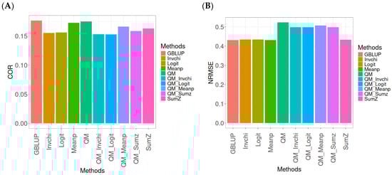
Figure 1.
Comparative performance of genomic prediction methods in terms of Pearson’s correlation (COR) (A) and normalized root mean square error (NRMSE) (B) for Disease dataset.
The analysis of Pearson’s correlation between observed and predicted values (Figure 1A) for the Disease dataset reveals that the GBLUP method stands out as the most effective approach, achieving a correlation of 0.1766, which is 0.8567% greater than QM’s correlation of 0.1751. In comparison to other methods, GBLUP significantly outperforms Meanp (0.1728, 2.1991% less effective), QM_Meanp (0.1661, 6.3215% less effective), SumZ (0.1630, 8.3436% less effective), QM_Sumz (0.1586, 11.3493% less effective), Logit (0.1559, 13.2777% less effective), Invchi (0.1552, 13.7887% less effective), QM_Invchi (0.1530, 15.4248% less effective), and QM_Logit (0.1528, 15.5759% less effective).
Regarding the NRMSE metric between observed and predicted values (Figure 1B) for the Disease dataset, the results indicate that the GBLUP method achieves the lowest average NRMSE, making it the most effective option. GBLUP yields a value of 0.4313, which is 0.1159% better than Meanp (0.4318) and 0.5565% better than SumZ (0.4337). Additionally, GBLUP outperforms Logit (0.4345) by 0.7419% and Invchi (0.4346) by 0.7651%. Notably, GBLUP also shows significant advantages over QM_Logit (0.4984) by 15.5576%, QM_Invchi (0.4986) by 15.604%, QM_Sumz (0.4987) by 15.6272%, QM_Meanp (0.5072) by 17.598%, and QM (0.5234) by 21.354%.
Overall, the analysis of the Disease dataset indicates that the GBLUP method is the most effective approach, demonstrating a higher Pearson’s correlation compared to other methods, including QM and Meanp. This trend is also reflected in the NRMSE metric, where GBLUP achieves the lowest average NRMSE, confirming its superior performance. Its advantages over a range of alternative methods, including various quantile mapping strategies, further solidify the reliability and effectiveness of GBLUP for predictive tasks in this context.
2.2. EYT_1
The results for the models evaluated on the EYT_1 dataset (Figure 2) were assessed using the same metrics, COR and NRMSE. For more details, see Table A2 (in Appendix A).
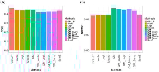
Figure 2.
Comparative performance of genomic prediction methods in terms of Pearson’s correlation (COR) (A) and normalized root mean square error (NRMSE) (B) for EYT_1 dataset.
The evaluation of Pearson’s correlation between observed and predicted values (Figure 2A) for the EYT_1 dataset indicates that the GBLUP method emerges as the most effective strategy, attaining a correlation of 0.4659, which is 3.9955% greater than Meanp’s correlation of 0.4480. In relation to other approaches, GBLUP significantly surpasses QM (0.4429, 5.193% less effective), Invchi (0.4417, 5.4788% less effective), Logit (0.4414, 5.5505% less effective), SumZ (0.4389, 6.1517% less effective), QM_Meanp (0.4273, 9.0335% less effective), QM_Sumz (0.4270, 9.1101% less effective), QM_Logit (0.4257, 9.4433% less effective), and QM_Invchi (0.4193, 11.1138% less effective).
Regarding the NRMSE metric between observed and predicted values (Figure 2B) for the EYT_1 dataset, the findings reveal that the GBLUP method achieves the lowest average NRMSE, establishing it as the most effective choice. GBLUP has a value of 0.0450, which is 0.8889% greater than Meanp (0.0454) and 1.1111% better than Invchi (0.0455). Additionally, GBLUP outperforms Logit (0.0456) and SumZ (0.0456) by 1.3333%. Notably, GBLUP also exhibits significant advantages over QM_Sumz (0.0512) by 13.7778%, QM_Logit (0.0519) by 15.3333%, QM_Invchi (0.0533) by 18.4444%, QM_Meanp (0.0534) by 18.6667%, and QM (0.0545) by 21.1111%.
Overall, the analysis of the EYT_1 dataset indicates that the GBLUP method consistently outperforms other strategies, displaying both the highest Pearson’s correlation and the lowest NRMSE. This establishes GBLUP as the most effective choice compared to Meanp, Invchi, and the various quantile mapping methods. Its superior performance across both metrics underscores its reliability and potential for the enhancement of predictive accuracy in related applications.
2.3. Wheat_1
This section presents the results of the genomic prediction models evaluated on the Wheat_1 data, considering the same metrics as before. For more details, see Table A3 (in Appendix A).
The assessment of Pearson’s correlation between observed and predicted values (Figure 3A) for the Wheat_1 dataset shows that the GBLUP method emerges as the most effective strategy, achieving a correlation of 0.4682, which is 3.8598% greater than Meanp’s correlation of 0.4406. In comparison to other methods, GBLUP significantly outperforms QM (0.4508, 6.2642% less effective), SumZ (0.4400, 6.4091% less effective), Logit (0.4387, 6.7244% less effective), Invchi (0.4314, 8.5304% less effective), QM_Meanp (0.4299, 8.909% less effective), QM_Invchi (0.4256, 10.0094% less effective), QM_Sumz (0.4214, 11.1058% less effective), and QM_Logit (0.4187, 11.8223% less effective).
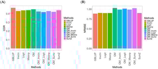
Figure 3.
Comparative performance of genomic prediction methods in terms of Pearson’s correlation (COR) (A) and normalized root mean square error (NRMSE) (B) for Wheat_1 dataset.
Regarding the NRMSE metric between observed and predicted values (Figure 3B) for the Wheat_1 dataset, the findings indicate that the GBLUP method achieves the lowest average NRMSE, establishing it as the most effective option. GBLUP has a value of 0.887, which is 1.5671% better than Logit (0.9009) and 1.6347% greater than Meanp (0.9015). Additionally, GBLUP outperforms SumZ (0.9016) by 1.646% and Invchi (0.9047) by 1.9955%. Notably, GBLUP also presents significant advantages over QM_Invchi (0.9866) by 11.2289%, QM_Meanp (0.9895) by 11.5558%, QM_Logit (1.0148) by 14.4081%, QM_Sumz (1.0238) by 15.4228%, and QM (1.0293) by 16.0428%.
The assessment of the Wheat_1 dataset reveals that the GBLUP method is the most effective strategy, achieving a higher Pearson’s correlation compared to other approaches, including Meanp and remaining methods. The performance of GBLUP is not only superior in correlation but also presents the lowest average NRMSE, further establishing its effectiveness. It significantly outperforms other methods, such as Logit and SumZ, as well as a range of quantile mapping strategies, indicating its reliability for predictive tasks. Overall, the consistent advantages of GBLUP reinforce its position as the preferred method in this context.
2.4. Across Data
In this section, the analysis of the results presented across datasets is given under the same model and metrics as before. For more details, see Table A4 (in Appendix A).
The assessment of Pearson’s correlation between observed and predicted values (Figure 4A) across datasets highlights the GBLUP method as the most effective strategy, achieving a correlation of 0.4834, which is 3.9794% greater than Meanp’s correlation of 0.4649. In comparison to other methods, GBLUP significantly outperforms QM (0.4659, 3.7562% less effective), SumZ (0.4584, 5.4538% less effective), Logit (0.4569, 5.8% less effective), and Invchi (0.4533, 6.6402% less effective). Notably, GBLUP also shows advantages over various quantile mapping methods, including QM_Meanp (0.4458, 8.4343% less effective), QM_Logit (0.4412, 9.5648% less effective), QM_Sumz (0.4405, 9.7389% less effective), and QM_Invchi (0.4355, 10.9989% less effective).
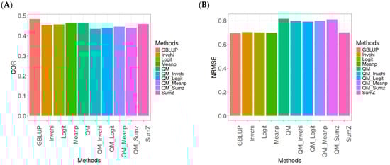
Figure 4.
Comparative performance of genomic prediction methods in terms of Pearson’s correlation (COR) (A) and normalized root mean square error (NRMSE) (B) across datasets, using quantile mapping.
The assessment of the NRMSE metric between observed and predicted values (Figure 4B) across datasets indicates that the GBLUP method achieves the lowest average NRMSE, establishing it as the most effective option. GBLUP has a value of 0.6954, which is 0.7046% better than Meanp (0.7003) and 0.9347% greater than SumZ (0.7019). Additionally, GBLUP outperforms Logit (0.7019) and Invchi (0.7043) by 0.9347% and 1.2798%, respectively. Notably, GBLUP also presents significant advantages over various quantile mapping methods, including QM_Logit (0.7928) by 14.0063%, QM_Meanp (0.7976) by 14.6966%, QM_Invchi (0.8018) by 15.3005%, QM_Sumz (0.8110) by 16.6235%, and QM (0.8160) by 17.3425%.
The assessment of Pearson’s correlation across datasets reveals that the GBLUP method is the most effective approach, achieving a higher correlation compared to other methods, including Meanp and various quantile mapping strategies. GBLUP not only excels in correlation but also records the lowest average NRMSE, solidifying its status as the most reliable option. Its performance surpasses that of Logit and SumZ, as well as several quantile mapping methods, indicating a clear advantage. Overall, GBLUP’s consistent effectiveness across both metrics reinforces its preference for predictive tasks in this context.
3. Discussion
The successful implementation of GS in plant breeding faces several challenges, including the need for high-quality genomic and phenotypic data, appropriate statistical models, and robust validation strategies. One key hurdle is the limited availability of large, diverse datasets required to capture the genetic architecture of complex traits and account for genotype-by-environment interactions, which are critical in breeding programs targeting multiple environments [,]. Additionally, computational demands increase significantly with the inclusion of high-dimensional genomic data, requiring advancements in algorithms and computational resources. Another challenge lies in translating GP predictions into actionable breeding decisions, demanding integration with traditional breeding practices and decision-support tools []. Addressing these issues involves interdisciplinary collaboration and significant investment in training, data curation, and infrastructure to fully leverage the potential of GP in enhancing genetic gains and breeding efficiency.
Improving the efficiency of GS in plant breeding relies on strategies that enhance prediction accuracy, optimize resource allocation, and integrate GS into breeding pipelines. One successful approach is the use of multi-environment trials (MET) to capture genotype-by-environment interactions, enabling better predictions across diverse target environments []. Sparse testing schemes, which involve phenotyping only a subset of genotypes in certain environments, are also effective in reducing costs while maintaining prediction accuracy when paired with robust statistical models [,]. Additionally, leveraging complementary data sources such as high-throughput phenotyping and environmental covariates can further enhance GS accuracy by providing insights into complex trait architectures []. Implementing these strategies requires investment in advanced data management systems and interdisciplinary collaboration to fully integrate GS into breeding programs and maximize genetic gains.
Despite its potential, the practical application of GS in plant breeding remains highly challenging due to complexities such as the need for high-quality genomic and phenotypic data, the variability in genotype-by-environment interactions, and the computational burden of analyzing large datasets. The effectiveness of GS often depends on the accuracy of prediction models, which can be hindered by limited training data, especially for less-studied traits or environments []. Furthermore, the integration of GS into breeding programs requires adapting existing workflows and overcoming economic and logistical barriers, such as the cost of genotyping and the need for skilled personnel []. To address these limitations, researchers are actively exploring novel approaches, including integrating environmental data, leveraging machine learning techniques, and developing strategies like sparse testing to improve the efficiency and scalability of GS []. These efforts aim to refine GS methodologies and make them more applicable to real-world breeding scenarios.
For this reason, this study explored the use of quantile mapping and the removal of outlier observations within a GBLUP framework to improve the predictive accuracy of the conventional GBLUP model. In theory, these combinations have the potential to enhance the prediction accuracy of GBLUP by addressing critical issues such as the influence of extreme values and non-normality in the data. Quantile mapping, by transforming the distribution of predictions to better align with observed values, can correct systematic biases that often undermine model performance. Simultaneously, outlier removal helps reduce noise and ensures that the model focuses on patterns representative of the majority of the data, which is particularly important when dealing with genomic data characterized by high dimensionality and complex interactions. These adjustments aim to refine the training dataset and statistical assumptions of the model, ultimately resulting in more robust and reliable predictions. Furthermore, integrating these strategies within the GBLUP framework offers an opportunity to adapt this widely used genomic prediction method to varying data qualities and environmental conditions, addressing persistent challenges in plant breeding programs.
However, our results combining the GBLUP method with quantile mapping and outlier detection techniques did not meet expectations. In terms of Pearson’s correlation, across all datasets and within each individual dataset, the GBLUP method proved to be the most effective, consistently achieving higher correlations than the alternative approaches. This superior performance of GBLUP is further supported by its ability to minimize errors, as evidenced by lower NRMSE values. Compared to other methods, including any outlier detection method, quantile mapping, and resulting combinations of quantile mapping with outlier detection techniques, GBLUP consistently delivers more accurate predictions, reaffirming its reliability and robustness in the context of breeding programs.
Our results emphasize the benefits and robustness of the GBLUP method, which remains one of the most popular approaches for genomic prediction. Its popularity stems from several key factors. Firstly, GBLUP is computationally efficient and relatively simple to implement, making it accessible for a wide range of breeding programs. Secondly, it leverages genomic relationships to predict breeding values, effectively capturing additive genetic effects, which are crucial for many quantitative traits. Additionally, GBLUP is grounded in a solid statistical framework, offering reliable and interpretable results. Its ability to handle high-dimensional genomic data without overfitting further contributes to its widespread use. Moreover, the compatibility of GBLUP with extensions, such as the incorporation of environmental covariates or non-additive effects, enhances its adaptability to complex breeding scenarios. These advantages collectively solidify the position of GBLUP as a cornerstone method in genomic prediction.
Finally, we want to emphasize that our results are specific to the datasets used in this study, which reflect genetic and environmental conditions. The observed lack of improvement in predictive accuracy when combining GBLUP with quantile mapping and outlier detection techniques may be influenced by the nature of the datasets, such as their size, genetic architecture, or level of noise. While these combinations did not outperform the conventional GBLUP method in this context, it is important to acknowledge that their effectiveness could vary under different circumstances. For instance, in datasets with pronounced outliers or non-normal distributions, quantile mapping and outlier removal may play a more significant role in improving model performance. Additionally, these techniques might offer advantages in scenarios in which specific traits exhibit strong non-linear patterns or in which genotype-by-environment interactions are highly complex. Therefore, while our findings reaffirm the robustness of the standard GBLUP method, they also suggest the need for further exploration of these combinations across diverse datasets to fully understand their potential.
This study evaluates the impact of quantile mapping and outlier detection on the accuracy of genomic predictions using GBLUP. However, confidence intervals for accuracy metrics, such as Pearson’s correlation and root means square error, were not computed, which limits the ability to assess the statistical uncertainty associated with the observed improvements. Additionally, formal hypothesis testing, such as paired statistical tests to compare GBLUP with and without these enhancements, was not conducted. While the study primarily focused on practical predictive improvements rather than statistical inference, future research should incorporate bootstrapping or cross-validation techniques to estimate confidence intervals and apply appropriate statistical tests, such as paired t-tests or Wilcoxon signed-rank tests, to determine whether the observed differences are statistically significant. Implementing these approaches would strengthen the robustness of the conclusions and provide a clearer understanding of the reliability and generalizability of the proposed methods across different datasets and breeding populations.
Furthermore, computational time was not systematically evaluated, which is an important factor when implementing these methods in large-scale genomic selection programs. Future studies should assess the trade-off between improved prediction accuracy and the additional computational cost associated with quantile mapping and outlier detection, particularly in large datasets where efficiency is a key consideration. Implementing these approaches would strengthen the robustness of the conclusions and provide a clearer understanding of the reliability, scalability, and generalizability of the proposed methods across different datasets and breeding populations.
4. Methods and Materials
4.1. Datasets
A detailed overview of the 14 datasets used in this study is provided in Table 1.

Table 1.
Brief data description. RCBD denotes randomized complete block design, while alpha-lattice denotes the alpha lattice experimental design.
4.2. Bayesian GBLUP Model
The GBLUP model implemented was:
where represents the best linear unbiased estimates (BLUE) for the i-th genotype. The grand mean is denoted by μ, and the random effects associated with genotypes (Lines), , is distributed as , where is the genomic relationship-matrix [] and is the genetic variance component. The residual errors, are assumed to be independent and normally distributed with mean 0 and variance . This model was implemented in R statistical software version 4.4.3 [] with the BGLR library of Pérez and de los Campos [].
4.3. Quantile Mapping (QM)
QM is a widely used bias adjustment technique for post-processing climate model simulations. It addresses the mismatch between the coarse spatial resolution of model outputs and finer spatial scales of interest []. QM achieves this by aligning the cumulative density function (CDF) of the modeled data with that of reference data for each target location. Specifically, it creates a quantile-dependent correction function to map simulated quantiles to their corresponding reference values. This correction function is then applied to the modeled time series, yielding bias-adjusted values that align with the distribution of the reference data. QM operates under the assumption that the CDF of a variable in the forecast and observational time series remains consistent in future periods []. Given variable x, QM minimizes discrepancies between the CDFs of model data and reference data over a calibration period. In practice, the algorithm maps the model output x to the observational output y using a transformation function ℎ, ensuring the two CDFs become equivalent []. In terms of equations, this results in:
where is the inverse function of the CDF. From Equation (1) it becomes clear that QM equates the cumulative distribution functions (CDFs) and respectively, of the observed data and modeled data , over a historical period, which results in the transfer function (1). The implemented QM scheme was based on the R package map version 3.4.2.1 [].
Since the QM method relies on the observed and predicted values from the training set to adjust predictions, it is important to emphasize that QM is specifically implemented to refine the predicted values generated by the GBLUP method. In other words, the conventional GBLUP results are enhanced through this QM adjustment process.
4.4. Outlier Detection Methods
The four methods used for the detection of influential measures are based on the p-value-based meta-analysis approach proposed by Budhlakoti and Mishra []. A brief description of these approaches is as follows. Let us assume there are K independent tests, and their corresponding p-values are , ,…,. Under , it is assumed that p-values from different methods (for individual observations) are uniformly distributed between 0 and 1 (i.e., ). To determine the overall statistical significance of the hypothesis under test ( i.e., null hypothesis vs. alternative hypothesis), individual p-values for each observation/genotype from different methods are combined. The specific methods used for this purpose are summarized in Table 2.
Table 2.
Outlier detection methods that combine p-values to calculate overall significance, where: denotes the statistical significance value from kth methods for an individual or genotype; K: different methods for which p-values can be combined; df: degrees of freedom; N: normal distribution; t: central t-distribution; χ2: central Chi-square distribution.
This approach (Table 2) was used to compute the final statistical significance values, specifically the combined p-values for the selected observations or genotypes. Influential observations were determined by applying a suitable p-value threshold. The methods were implemented using source code available from a GitHub repository at GitHub—BudhlakotiN/OGS: R/OGS: Outlier in Genomics Data.
It is important to note that these four outlier detection methods (Invchi, Logit, Meanp, SumZ) were applied to the training set of each fold. After implementation, any observations identified as outliers were removed from the training set. The reduced training set was then used to implement the GBLUP method, as described in Equation (1).
4.5. Combining Quantile Mapping with Outlier Detection Methods Using GBLUP
Combining the quantile mapping (QM) method with the four outlier detection methods (Invchi, Logit, Meanp, and SumZ) resulted in the development of four additional approaches, denoted as QM_Invchi, QM_Logit, QM_Meanp, and QM_SumZ. These methods were implemented as follows: first, each of the four outlier detection methods was applied as previously described. Subsequently, the QM method was applied using the observed and predicted values from the training set produced by each of the four outlier detection methods.
Therefore, a total of 10 models were employed in this study. These included: GBLUP alone; GBLUP combined with quantile mapping (QM); GBLUP combined with the four outlier detection methods, Invchi, Logit, Meanp, and SumZ; and, finally, GBLUP combined with the four combinations of quantile mapping (QM) with the outlier detection methods (QM_Invchi, QM_Logit, QM_Meanp, and QM_SumZ). Results are thus presented for a total of 10 combinations of GBLUP-based models, incorporating various combinations with QM and outlier detection methods.
4.6. Evaluation of Prediction Performance
To evaluate the proposed methods, we used cross-validation; more specifically, a 10-fold cross-validation approach. In each fold, 80% of the data were allocated for training and 20% for testing. For each testing set, prediction accuracy was assessed using two metrics: average Pearson’s correlation (COR) and normalized root mean square error (NRMSE) []. These metrics were selected because they facilitate comparisons across different traits, being independent of the trait’s scale. Both metrics were calculated using the observed values () and the predicted values [] from the testing set of each fold. The average performance over the 10 folds was reported. COR and NRMSE were selected not only for their utility in genomic prediction but also because they are widely used metrics for the evaluation of prediction performance.
5. Conclusions
Our benchmark analysis shows that the conventional GBLUP method outperforms quantile mapping, outlier detection techniques, and their combination in the context of genomic prediction. These findings reaffirm the effectiveness and robustness of GBLUP, which remains one of the most widely used techniques in plant and animal breeding for genomic selection. However, our results are not definitive, as substantial empirical evidence suggests that removing outliers from the training data can enhance prediction accuracy and quantile mapping can improve predictions in the testing set. Therefore, further empirical evaluations are essential to thoroughly assess the benefits and limitations of these alternative methods within the context of genomic selection. This will provide a more comprehensive understanding of their potential to complement or improve upon GBLUP.
Author Contributions
Conceptualization, O.A.M.-L. and A.M.-L.; methodology, O.A.M.-L. and A.M.-L.; validation and investigation, O.A.M.-L., A.M.-L., A.A. and J.C.; writing—original draft preparation and software, A.A. and R.B.-M.; writing—review and editing, A.C. Authors P.V., G.G., L.C.-H., S.D., C.S.P. and L.G.P. have read the first version. All authors have read and agreed to the published version of the manuscript.
Funding
This research was funded by SLU Grogrund grant number SLU.ltv.2020.1.1.1-654.
Institutional Review Board Statement
Not applicable.
Informed Consent Statement
Not applicable.
Data Availability Statement
The genomic and phenotypic data used in this study are available at the following link. https://github.com/osval78/Refaning_Penalized_Regression, accessed on 8 January 2025.
Conflicts of Interest
The authors declare no conflicts of interest.
Abbreviations
| GS | Genomic selection |
| GBLUP | Genomic best linear unbiased predictor |
| QM | Quantile mapping |
| CDF | Cumulative density function |
| COR | Correlation |
| NRMSE | Normalized root mean square error |
Appendix A
Results for datasets Disease (Table A1), EYT_1 (Table A2), Wheat_1 (Table A3), and across datasets (Table A4).
Table A1.
Performance comparison of genomic prediction methods in terms of Pearson’s correlation (COR) (A) and the normalized root mean square error (NRMSE) (B) for the Disease dataset, using quantile mapping.
Table A1.
Performance comparison of genomic prediction methods in terms of Pearson’s correlation (COR) (A) and the normalized root mean square error (NRMSE) (B) for the Disease dataset, using quantile mapping.
| Metric | Method | Min | Mean | Median | Max |
|---|---|---|---|---|---|
| COR | GBLUP | 0.0976 | 0.1766 | 0.1977 | 0.2344 |
| COR | Invchi | 0.0544 | 0.1552 | 0.1820 | 0.2293 |
| COR | Logit | 0.0506 | 0.1559 | 0.1829 | 0.2344 |
| COR | Meanp | 0.1008 | 0.1728 | 0.1755 | 0.2421 |
| COR | QM | 0.1018 | 0.1751 | 0.1882 | 0.2351 |
| COR | QM_Invchi | 0.0511 | 0.1530 | 0.1844 | 0.2234 |
| COR | QM_Logit | 0.0486 | 0.1528 | 0.1841 | 0.2258 |
| COR | QM_Meanp | 0.0842 | 0.1661 | 0.1735 | 0.2407 |
| COR | QM_Sumz | 0.0699 | 0.1586 | 0.1855 | 0.2204 |
| COR | SumZ | 0.0681 | 0.1630 | 0.1917 | 0.2291 |
| COR_SE | GBLUP | 0.0169 | 0.0234 | 0.0242 | 0.0290 |
| COR_SE | Invchi | 0.0276 | 0.0309 | 0.0323 | 0.0327 |
| COR_SE | Logit | 0.0221 | 0.0317 | 0.0341 | 0.0388 |
| COR_SE | Meanp | 0.0247 | 0.0272 | 0.0252 | 0.0318 |
| COR_SE | QM | 0.0206 | 0.0247 | 0.0228 | 0.0307 |
| COR_SE | QM_Invchi | 0.0303 | 0.0326 | 0.0323 | 0.0352 |
| COR_SE | QM_Logit | 0.0227 | 0.0320 | 0.0328 | 0.0407 |
| COR_SE | QM_Meanp | 0.0241 | 0.0267 | 0.0241 | 0.0318 |
| COR_SE | QM_Sumz | 0.0201 | 0.0282 | 0.0306 | 0.0340 |
| COR_SE | SumZ | 0.0200 | 0.0274 | 0.0295 | 0.0327 |
| NRMSE | GBLUP | 0.4055 | 0.4313 | 0.4127 | 0.4757 |
| NRMSE | Invchi | 0.4066 | 0.4346 | 0.4136 | 0.4837 |
| NRMSE | Logit | 0.4060 | 0.4345 | 0.4135 | 0.4840 |
| NRMSE | Meanp | 0.4044 | 0.4318 | 0.4149 | 0.4761 |
| NRMSE | QM | 0.4670 | 0.5234 | 0.5028 | 0.6005 |
| NRMSE | QM_Invchi | 0.4464 | 0.4986 | 0.4728 | 0.5767 |
| NRMSE | QM_Logit | 0.4439 | 0.4984 | 0.4750 | 0.5762 |
| NRMSE | QM_Meanp | 0.4464 | 0.5072 | 0.4954 | 0.5798 |
| NRMSE | QM_Sumz | 0.4463 | 0.4987 | 0.4741 | 0.5756 |
| NRMSE | SumZ | 0.4063 | 0.4337 | 0.4127 | 0.4820 |
| NRMSE_SE | GBLUP | 0.0032 | 0.0063 | 0.0065 | 0.0092 |
| NRMSE_SE | Invchi | 0.0039 | 0.0066 | 0.0064 | 0.0095 |
| NRMSE_SE | Logit | 0.0043 | 0.0065 | 0.0058 | 0.0093 |
| NRMSE_SE | Meanp | 0.0036 | 0.0062 | 0.0058 | 0.0093 |
| NRMSE_SE | QM | 0.0076 | 0.0091 | 0.0090 | 0.0107 |
| NRMSE_SE | QM_Invchi | 0.0077 | 0.0100 | 0.0105 | 0.0119 |
| NRMSE_SE | QM_Logit | 0.0069 | 0.0089 | 0.0099 | 0.0101 |
| NRMSE_SE | QM_Meanp | 0.0076 | 0.0102 | 0.0111 | 0.0118 |
| NRMSE_SE | QM_Sumz | 0.0059 | 0.0091 | 0.0098 | 0.0116 |
| NRMSE_SE | SumZ | 0.0043 | 0.0066 | 0.0062 | 0.0093 |
Table A2.
Performance comparison of genomic prediction methods in terms of Pearson’s correlation (COR) (A) and the normalized root mean square error (NRMSE) (B) for the EYT_1 dataset, using quantile mapping.
Table A2.
Performance comparison of genomic prediction methods in terms of Pearson’s correlation (COR) (A) and the normalized root mean square error (NRMSE) (B) for the EYT_1 dataset, using quantile mapping.
| Metric | Method | Min | Mean | Median | Max |
|---|---|---|---|---|---|
| COR | GBLUP | 0.4282 | 0.4659 | 0.4727 | 0.4901 |
| COR | Invchi | 0.4037 | 0.4417 | 0.4445 | 0.4741 |
| COR | Logit | 0.3937 | 0.4414 | 0.4477 | 0.4765 |
| COR | Meanp | 0.4028 | 0.4480 | 0.4570 | 0.4753 |
| COR | QM | 0.3542 | 0.4429 | 0.4633 | 0.4908 |
| COR | QM_Invchi | 0.3588 | 0.4193 | 0.4283 | 0.4617 |
| COR | QM_Logit | 0.3715 | 0.4257 | 0.4306 | 0.4698 |
| COR | QM_Meanp | 0.3393 | 0.4273 | 0.4477 | 0.4746 |
| COR | QM_Sumz | 0.3794 | 0.4270 | 0.4292 | 0.4702 |
| COR | SumZ | 0.3963 | 0.4389 | 0.4438 | 0.4717 |
| COR_SE | GBLUP | 0.0096 | 0.0164 | 0.0151 | 0.0256 |
| COR_SE | Invchi | 0.0162 | 0.0196 | 0.0178 | 0.0264 |
| COR_SE | Logit | 0.0153 | 0.0184 | 0.0181 | 0.0220 |
| COR_SE | Meanp | 0.0126 | 0.0179 | 0.0167 | 0.0257 |
| COR_SE | QM | 0.0109 | 0.0234 | 0.0197 | 0.0432 |
| COR_SE | QM_Invchi | 0.0193 | 0.0279 | 0.0291 | 0.0339 |
| COR_SE | QM_Logit | 0.0156 | 0.0226 | 0.0233 | 0.0284 |
| COR_SE | QM_Meanp | 0.0122 | 0.0226 | 0.0222 | 0.0338 |
| COR_SE | QM_Sumz | 0.0120 | 0.0225 | 0.0236 | 0.0308 |
| COR_SE | SumZ | 0.0126 | 0.0190 | 0.0191 | 0.0252 |
| NRMSE | GBLUP | 0.0349 | 0.0450 | 0.0448 | 0.0552 |
| NRMSE | Invchi | 0.0355 | 0.0455 | 0.0455 | 0.0557 |
| NRMSE | Logit | 0.0354 | 0.0456 | 0.0456 | 0.0556 |
| NRMSE | Meanp | 0.0353 | 0.0454 | 0.0453 | 0.0558 |
| NRMSE | QM | 0.0386 | 0.0545 | 0.0575 | 0.0646 |
| NRMSE | QM_Invchi | 0.0428 | 0.0533 | 0.0538 | 0.0628 |
| NRMSE | QM_Logit | 0.0377 | 0.0519 | 0.0536 | 0.0629 |
| NRMSE | QM_Meanp | 0.0376 | 0.0534 | 0.0571 | 0.0617 |
| NRMSE | QM_Sumz | 0.0380 | 0.0512 | 0.0522 | 0.0626 |
| NRMSE | SumZ | 0.0355 | 0.0456 | 0.0456 | 0.0558 |
| NRMSE_SE | GBLUP | 0.0004 | 0.0006 | 0.0006 | 0.0010 |
| NRMSE_SE | Invchi | 0.0005 | 0.0008 | 0.0008 | 0.0011 |
| NRMSE_SE | Logit | 0.0006 | 0.0008 | 0.0007 | 0.0012 |
| NRMSE_SE | Meanp | 0.0006 | 0.0008 | 0.0008 | 0.0010 |
| NRMSE_SE | QM | 0.0003 | 0.0031 | 0.0023 | 0.0076 |
| NRMSE_SE | QM_Invchi | 0.0010 | 0.0040 | 0.0043 | 0.0064 |
| NRMSE_SE | QM_Logit | 0.0006 | 0.0033 | 0.0038 | 0.0049 |
| NRMSE_SE | QM_Meanp | 0.0006 | 0.0032 | 0.0024 | 0.0074 |
| NRMSE_SE | QM_Sumz | 0.0006 | 0.0026 | 0.0024 | 0.0049 |
| NRMSE_SE | SumZ | 0.0006 | 0.0008 | 0.0007 | 0.0010 |
Table A3.
Performance comparison of genomic prediction methods in terms of Pearson’s correlation (COR) (A) and the normalized root mean square error (NRMSE) (B) for the Wheat_1 dataset, using quantile mapping.
Table A3.
Performance comparison of genomic prediction methods in terms of Pearson’s correlation (COR) (A) and the normalized root mean square error (NRMSE) (B) for the Wheat_1 dataset, using quantile mapping.
| Metric | Method | Min | Mean | Median | Max |
|---|---|---|---|---|---|
| COR | GBLUP | 0.4682 | 0.4682 | 0.4682 | 0.4682 |
| COR | Invchi | 0.4314 | 0.4314 | 0.4314 | 0.4314 |
| COR | Logit | 0.4387 | 0.4387 | 0.4387 | 0.4387 |
| COR | Meanp | 0.4406 | 0.4406 | 0.4406 | 0.4406 |
| COR | QM | 0.4508 | 0.4508 | 0.4508 | 0.4508 |
| COR | QM_Invchi | 0.4256 | 0.4256 | 0.4256 | 0.4256 |
| COR | QM_Logit | 0.4187 | 0.4187 | 0.4187 | 0.4187 |
| COR | QM_Meanp | 0.4299 | 0.4299 | 0.4299 | 0.4299 |
| COR | QM_Sumz | 0.4214 | 0.4214 | 0.4214 | 0.4214 |
| COR | SumZ | 0.4400 | 0.4400 | 0.4400 | 0.4400 |
| COR_SE | GBLUP | 0.0149 | 0.0149 | 0.0149 | 0.0149 |
| COR_SE | Invchi | 0.0116 | 0.0116 | 0.0116 | 0.0116 |
| COR_SE | Logit | 0.0123 | 0.0123 | 0.0123 | 0.0123 |
| COR_SE | Meanp | 0.0122 | 0.0122 | 0.0122 | 0.0122 |
| COR_SE | QM | 0.0175 | 0.0175 | 0.0175 | 0.0175 |
| COR_SE | QM_Invchi | 0.0161 | 0.0161 | 0.0161 | 0.0161 |
| COR_SE | QM_Logit | 0.0129 | 0.0129 | 0.0129 | 0.0129 |
| COR_SE | QM_Meanp | 0.0137 | 0.0137 | 0.0137 | 0.0137 |
| COR_SE | QM_Sumz | 0.0166 | 0.0166 | 0.0166 | 0.0166 |
| COR_SE | SumZ | 0.0127 | 0.0127 | 0.0127 | 0.0127 |
| NRMSE | GBLUP | 0.8870 | 0.8870 | 0.8870 | 0.8870 |
| NRMSE | Invchi | 0.9047 | 0.9047 | 0.9047 | 0.9047 |
| NRMSE | Logit | 0.9009 | 0.9009 | 0.9009 | 0.9009 |
| NRMSE | Meanp | 0.9015 | 0.9015 | 0.9015 | 0.9015 |
| NRMSE | QM | 1.0293 | 1.0293 | 1.0293 | 1.0293 |
| NRMSE | QM_Invchi | 0.9866 | 0.9866 | 0.9866 | 0.9866 |
| NRMSE | QM_Logit | 1.0148 | 1.0148 | 1.0148 | 1.0148 |
| NRMSE | QM_Meanp | 0.9895 | 0.9895 | 0.9895 | 0.9895 |
| NRMSE | QM_Sumz | 1.0238 | 1.0238 | 1.0238 | 1.0238 |
| NRMSE | SumZ | 0.9016 | 0.9016 | 0.9016 | 0.9016 |
| NRMSE_SE | GBLUP | 0.0092 | 0.0092 | 0.0092 | 0.0092 |
| NRMSE_SE | Invchi | 0.0053 | 0.0053 | 0.0053 | 0.0053 |
| NRMSE_SE | Logit | 0.0060 | 0.0060 | 0.0060 | 0.0060 |
| NRMSE_SE | Meanp | 0.0055 | 0.0055 | 0.0055 | 0.0055 |
| NRMSE_SE | QM | 0.0436 | 0.0436 | 0.0436 | 0.0436 |
| NRMSE_SE | QM_Invchi | 0.0367 | 0.0367 | 0.0367 | 0.0367 |
| NRMSE_SE | QM_Logit | 0.0363 | 0.0363 | 0.0363 | 0.0363 |
| NRMSE_SE | QM_Meanp | 0.0367 | 0.0367 | 0.0367 | 0.0367 |
| NRMSE_SE | QM_Sumz | 0.0461 | 0.0461 | 0.0461 | 0.0461 |
| NRMSE_SE | SumZ | 0.0059 | 0.0059 | 0.0059 | 0.0059 |
Table A4.
Performance comparison of genomic prediction methods in terms of Pearson’s correlation (COR) (A) and the normalized root mean square error (NRMSE) (B) across the datasets, using quantile mapping.
Table A4.
Performance comparison of genomic prediction methods in terms of Pearson’s correlation (COR) (A) and the normalized root mean square error (NRMSE) (B) across the datasets, using quantile mapping.
| Metric | Method | Min | Mean | Median | Max |
|---|---|---|---|---|---|
| COR | GBLUP | 0.0976 | 0.4834 | 0.4937 | 0.6941 |
| COR | Invchi | 0.0544 | 0.4533 | 0.4682 | 0.6667 |
| COR | Logit | 0.0506 | 0.4569 | 0.4728 | 0.6676 |
| COR | Meanp | 0.1008 | 0.4649 | 0.4751 | 0.6739 |
| COR | QM | 0.1018 | 0.4659 | 0.4805 | 0.6978 |
| COR | QM_Invchi | 0.0511 | 0.4355 | 0.4406 | 0.6653 |
| COR | QM_Logit | 0.0486 | 0.4412 | 0.4588 | 0.6668 |
| COR | QM_Meanp | 0.0842 | 0.4458 | 0.4593 | 0.6751 |
| COR | QM_Sumz | 0.0699 | 0.4405 | 0.4645 | 0.6633 |
| COR | SumZ | 0.0681 | 0.4584 | 0.4709 | 0.6662 |
| COR_SE | GBLUP | 0.0092 | 0.0200 | 0.0179 | 0.0503 |
| COR_SE | Invchi | 0.0107 | 0.0228 | 0.0197 | 0.0659 |
| COR_SE | Logit | 0.0073 | 0.0223 | 0.0199 | 0.0657 |
| COR_SE | Meanp | 0.0093 | 0.0222 | 0.0199 | 0.0605 |
| COR_SE | QM | 0.0109 | 0.0245 | 0.0225 | 0.0507 |
| COR_SE | QM_Invchi | 0.0140 | 0.0278 | 0.0246 | 0.0570 |
| COR_SE | QM_Logit | 0.0096 | 0.0255 | 0.0206 | 0.0668 |
| COR_SE | QM_Meanp | 0.0088 | 0.0265 | 0.0247 | 0.0550 |
| COR_SE | QM_Sumz | 0.0120 | 0.0256 | 0.0217 | 0.0502 |
| COR_SE | SumZ | 0.0097 | 0.0219 | 0.0191 | 0.0577 |
| NRMSE | GBLUP | 0.0297 | 0.6954 | 0.4210 | 7.9058 |
| NRMSE | Invchi | 0.0305 | 0.7043 | 0.4254 | 7.9443 |
| NRMSE | Logit | 0.0304 | 0.7019 | 0.4249 | 7.8848 |
| NRMSE | Meanp | 0.0300 | 0.7003 | 0.4236 | 7.8912 |
| NRMSE | QM | 0.0361 | 0.8160 | 0.4860 | 8.8085 |
| NRMSE | QM_Invchi | 0.0312 | 0.8018 | 0.4719 | 8.6206 |
| NRMSE | QM_Logit | 0.0377 | 0.7928 | 0.4765 | 8.6409 |
| NRMSE | QM_Meanp | 0.0376 | 0.7976 | 0.4829 | 8.6800 |
| NRMSE | QM_Sumz | 0.0380 | 0.8110 | 0.4701 | 8.6088 |
| NRMSE | SumZ | 0.0300 | 0.7019 | 0.4221 | 7.9065 |
| NRMSE_SE | GBLUP | 0.0004 | 0.0885 | 0.0064 | 2.7860 |
| NRMSE_SE | Invchi | 0.0005 | 0.0885 | 0.0063 | 2.7937 |
| NRMSE_SE | Logit | 0.0006 | 0.0882 | 0.0059 | 2.7865 |
| NRMSE_SE | Meanp | 0.0006 | 0.0878 | 0.0058 | 2.7730 |
| NRMSE_SE | QM | 0.0003 | 0.1316 | 0.0107 | 3.1423 |
| NRMSE_SE | QM_Invchi | 0.0010 | 0.1282 | 0.0104 | 3.0366 |
| NRMSE_SE | QM_Logit | 0.0006 | 0.1194 | 0.0102 | 3.0848 |
| NRMSE_SE | QM_Meanp | 0.0006 | 0.1295 | 0.0112 | 3.0857 |
| NRMSE_SE | QM_Sumz | 0.0006 | 0.1320 | 0.0124 | 3.0495 |
| NRMSE_SE | SumZ | 0.0006 | 0.0887 | 0.0063 | 2.8039 |
Appendix B
Figures for datasets Maize (Figure A1), Japonica (Figure A2), Indica (Figure A3), Groundnut (Figure A4), EYT_2 (Figure A5), EYT_3 (Figure A6), Wheat_2 (Figure A7), Wheat_3 (Figure A8), Wheat_4 (Figure A9), Wheat_5 (Figure A10), and Wheat_6 (Figure A11).
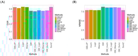
Figure A1.
Comparative performance of genomic prediction methods in terms of Pearson’s correlation (COR) (A) and the normalized root mean square error (NRMSE) (B) for the Maize dataset, using quantile mapping.
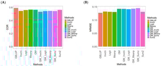
Figure A2.
Comparative performance of genomic prediction methods in terms of Pearson’s correlation (COR) (A) and the normalized root mean square error (NRMSE) (B) for the Japonica dataset, using quantile mapping.
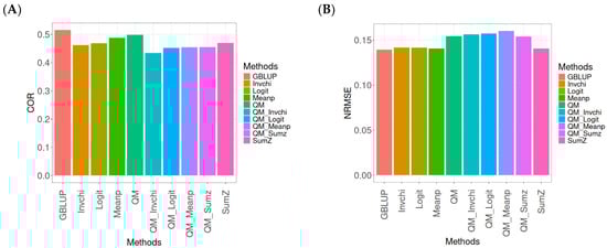
Figure A3.
Comparative performance of genomic prediction methods in terms of Pearson’s correlation (COR) (A) and the normalized root mean square error (NRMSE) (B) for the Indica dataset, using quantile mapping.
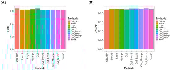
Figure A4.
Comparative performance of genomic prediction methods in terms of Pearson’s correlation (COR) (A) and the normalized root mean square error (NRMSE) (B) for the Groundnut dataset, using quantile mapping.
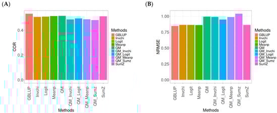
Figure A5.
Comparative performance of genomic prediction methods in terms of Pearson’s correlation (COR) (A) and the normalized root mean square error (NRMSE) (B) for the EYT_2 dataset, using quantile mapping.
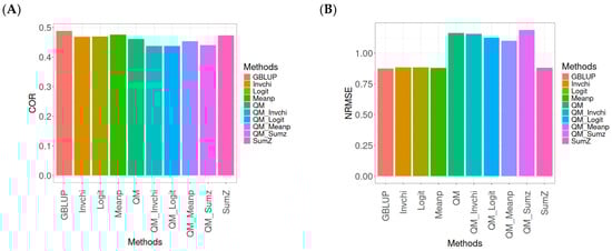
Figure A6.
Comparative performance of genomic prediction methods in terms of Pearson’s correlation (COR) (A) and the normalized root mean square error (NRMSE) (B) for the EYT_3 dataset, using quantile mapping.
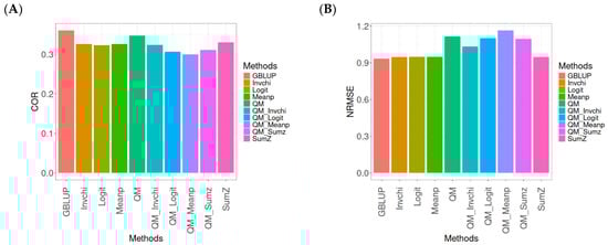
Figure A7.
Comparative performance of genomic prediction methods in terms of Pearson’s correlation (COR) (A) and the Normalized Root Mean Square Error (NRMSE) (B) for the Wheat_2 dataset, using quantile mapping.
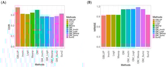
Figure A8.
Comparative performance of genomic prediction methods in terms of Pearson’s correlation (COR) (A) and the normalized root mean square error (NRMSE) (B) for the Wheat_3 dataset, using quantile mapping.
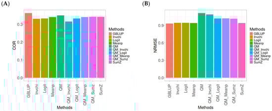
Figure A9.
Comparative performance of genomic prediction methods in terms of Pearson’s correlation (COR) (A) and the normalized root mean square error (NRMSE) (B) for the Wheat_4 dataset, using quantile mapping.
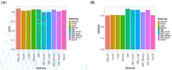
Figure A10.
Comparative performance of genomic prediction methods in terms of Pearson’s correlation (COR) (A) and the normalized root mean square error (NRMSE) (B) for the Wheat_5 dataset, using quantile mapping.
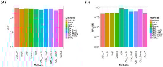
Figure A11.
Comparative performance of genomic prediction methods in terms of Pearson’s correlation (COR) (A) and the normalized root mean square error (NRMSE) (B) for the Wheat_6 dataset, using quantile mapping.
Appendix C
Table of results for datasets Maize, Japonica, Indica, Groundnut, EYT_2, EYT_3, Wheat_2, Wheat_3, Wheat_4, Wheat_5, and Wheat_6.
Table A5.
Comparative performance of genomic prediction models in terms of Pearson’s correlation (COR and COR standard error COR_SE) and the normalized root mean square error (NRMSE and NRMSE standard error, NRMSE_SE) for Maize, Japonica, Indica, Groundnut, EYT_2, EYT_3, Wheat_2, Wheat_3, Wheat_4, Wheat_5, and Wheat_6 datasets.
| Data | Metric | Method | Min | Mean | Median | Max |
|---|---|---|---|---|---|---|
| Maize | COR | GBLUP | 0.4225 | 0.4225 | 0.4225 | 0.4225 |
| Maize | COR | Invchi | 0.4106 | 0.4106 | 0.4106 | 0.4106 |
| Maize | COR | Logit | 0.4276 | 0.4276 | 0.4276 | 0.4276 |
| Maize | COR | Meanp | 0.4235 | 0.4235 | 0.4235 | 0.4235 |
| Maize | COR | QM | 0.3748 | 0.3748 | 0.3748 | 0.3748 |
| Maize | COR | QM_Invchi | 0.3691 | 0.3691 | 0.3691 | 0.3691 |
| Maize | COR | QM_Logit | 0.3809 | 0.3809 | 0.3809 | 0.3809 |
| Maize | COR | QM_Meanp | 0.3741 | 0.3741 | 0.3741 | 0.3741 |
| Maize | COR | QM_Sumz | 0.3792 | 0.3792 | 0.3792 | 0.3792 |
| Maize | COR | SumZ | 0.4264 | 0.4264 | 0.4264 | 0.4264 |
| Maize | COR_SE | GBLUP | 0.0180 | 0.0180 | 0.0180 | 0.0180 |
| Maize | COR_SE | Invchi | 0.0173 | 0.0173 | 0.0173 | 0.0173 |
| Maize | COR_SE | Logit | 0.0176 | 0.0176 | 0.0176 | 0.0176 |
| Maize | COR_SE | Meanp | 0.0174 | 0.0174 | 0.0174 | 0.0174 |
| Maize | COR_SE | QM | 0.0229 | 0.0229 | 0.0229 | 0.0229 |
| Maize | COR_SE | QM_Invchi | 0.0237 | 0.0237 | 0.0237 | 0.0237 |
| Maize | COR_SE | QM_Logit | 0.0201 | 0.0201 | 0.0201 | 0.0201 |
| Maize | COR_SE | QM_Meanp | 0.0218 | 0.0218 | 0.0218 | 0.0218 |
| Maize | COR_SE | QM_Sumz | 0.0206 | 0.0206 | 0.0206 | 0.0206 |
| Maize | COR_SE | SumZ | 0.0175 | 0.0175 | 0.0175 | 0.0175 |
| Maize | NRMSE | GBLUP | 7.9058 | 7.9058 | 7.9058 | 7.9058 |
| Maize | NRMSE | Invchi | 7.9443 | 7.9443 | 7.9443 | 7.9443 |
| Maize | NRMSE | Logit | 7.8848 | 7.8848 | 7.8848 | 7.8848 |
| Maize | NRMSE | Meanp | 7.8912 | 7.8912 | 7.8912 | 7.8912 |
| Maize | NRMSE | QM | 8.8085 | 8.8085 | 8.8085 | 8.8085 |
| Maize | NRMSE | QM_Invchi | 8.6206 | 8.6206 | 8.6206 | 8.6206 |
| Maize | NRMSE | QM_Logit | 8.6409 | 8.6409 | 8.6409 | 8.6409 |
| Maize | NRMSE | QM_Meanp | 8.6800 | 8.6800 | 8.6800 | 8.6800 |
| Maize | NRMSE | QM_Sumz | 8.6088 | 8.6088 | 8.6088 | 8.6088 |
| Maize | NRMSE | SumZ | 7.9065 | 7.9065 | 7.9065 | 7.9065 |
| Maize | NRMSE_SE | GBLUP | 2.7860 | 2.7860 | 2.7860 | 2.7860 |
| Maize | NRMSE_SE | Invchi | 2.7937 | 2.7937 | 2.7937 | 2.7937 |
| Maize | NRMSE_SE | Logit | 2.7865 | 2.7865 | 2.7865 | 2.7865 |
| Maize | NRMSE_SE | Meanp | 2.7730 | 2.7730 | 2.7730 | 2.7730 |
| Maize | NRMSE_SE | QM | 3.1423 | 3.1423 | 3.1423 | 3.1423 |
| Maize | NRMSE_SE | QM_Invchi | 3.0366 | 3.0366 | 3.0366 | 3.0366 |
| Maize | NRMSE_SE | QM_Logit | 3.0848 | 3.0848 | 3.0848 | 3.0848 |
| Maize | NRMSE_SE | QM_Meanp | 3.0857 | 3.0857 | 3.0857 | 3.0857 |
| Maize | NRMSE_SE | QM_Sumz | 3.0495 | 3.0495 | 3.0495 | 3.0495 |
| Maize | NRMSE_SE | SumZ | 2.8039 | 2.8039 | 2.8039 | 2.8039 |
| Japonica | COR | GBLUP | 0.5681 | 0.5914 | 0.5803 | 0.6366 |
| Japonica | COR | Invchi | 0.5266 | 0.5461 | 0.5412 | 0.5753 |
| Japonica | COR | Logit | 0.5372 | 0.5602 | 0.5602 | 0.5831 |
| Japonica | COR | Meanp | 0.5478 | 0.5662 | 0.5637 | 0.5896 |
| Japonica | COR | QM | 0.5246 | 0.5633 | 0.5691 | 0.5905 |
| Japonica | COR | QM_Invchi | 0.4955 | 0.5333 | 0.5320 | 0.5737 |
| Japonica | COR | QM_Logit | 0.5171 | 0.5430 | 0.5364 | 0.5821 |
| Japonica | COR | QM_Meanp | 0.5164 | 0.5473 | 0.5421 | 0.5884 |
| Japonica | COR | QM_Sumz | 0.5068 | 0.5430 | 0.5378 | 0.5895 |
| Japonica | COR | SumZ | 0.5376 | 0.5609 | 0.5580 | 0.5901 |
| Japonica | COR_SE | GBLUP | 0.0182 | 0.0233 | 0.0198 | 0.0352 |
| Japonica | COR_SE | Invchi | 0.0167 | 0.0279 | 0.0262 | 0.0426 |
| Japonica | COR_SE | Logit | 0.0201 | 0.0285 | 0.0272 | 0.0395 |
| Japonica | COR_SE | Meanp | 0.0218 | 0.0297 | 0.0270 | 0.0428 |
| Japonica | COR_SE | QM | 0.0187 | 0.0337 | 0.0328 | 0.0507 |
| Japonica | COR_SE | QM_Invchi | 0.0178 | 0.0278 | 0.0272 | 0.0390 |
| Japonica | COR_SE | QM_Logit | 0.0197 | 0.0370 | 0.0307 | 0.0668 |
| Japonica | COR_SE | QM_Meanp | 0.0217 | 0.0329 | 0.0319 | 0.0460 |
| Japonica | COR_SE | QM_Sumz | 0.0173 | 0.0301 | 0.0270 | 0.0490 |
| Japonica | COR_SE | SumZ | 0.0175 | 0.0287 | 0.0276 | 0.0422 |
| Japonica | NRMSE | GBLUP | 0.0297 | 0.1274 | 0.0524 | 0.3752 |
| Japonica | NRMSE | Invchi | 0.0305 | 0.1322 | 0.0546 | 0.3891 |
| Japonica | NRMSE | Logit | 0.0304 | 0.1313 | 0.0540 | 0.3869 |
| Japonica | NRMSE | Meanp | 0.0300 | 0.1303 | 0.0538 | 0.3837 |
| Japonica | NRMSE | QM | 0.0413 | 0.1427 | 0.0598 | 0.4100 |
| Japonica | NRMSE | QM_Invchi | 0.0312 | 0.1424 | 0.0606 | 0.4171 |
| Japonica | NRMSE | QM_Logit | 0.0409 | 0.1413 | 0.0558 | 0.4126 |
| Japonica | NRMSE | QM_Meanp | 0.0487 | 0.1430 | 0.0558 | 0.4117 |
| Japonica | NRMSE | QM_Sumz | 0.0392 | 0.1448 | 0.0622 | 0.4157 |
| Japonica | NRMSE | SumZ | 0.0300 | 0.1312 | 0.0541 | 0.3866 |
| Japonica | NRMSE_SE | GBLUP | 0.0010 | 0.0045 | 0.0030 | 0.0110 |
| Japonica | NRMSE_SE | Invchi | 0.0009 | 0.0049 | 0.0038 | 0.0110 |
| Japonica | NRMSE_SE | Logit | 0.0010 | 0.0047 | 0.0037 | 0.0106 |
| Japonica | NRMSE_SE | Meanp | 0.0009 | 0.0049 | 0.0038 | 0.0110 |
| Japonica | NRMSE_SE | QM | 0.0018 | 0.0078 | 0.0093 | 0.0107 |
| Japonica | NRMSE_SE | QM_Invchi | 0.0011 | 0.0054 | 0.0051 | 0.0102 |
| Japonica | NRMSE_SE | QM_Logit | 0.0016 | 0.0066 | 0.0072 | 0.0103 |
| Japonica | NRMSE_SE | QM_Meanp | 0.0017 | 0.0073 | 0.0078 | 0.0118 |
| Japonica | NRMSE_SE | QM_Sumz | 0.0018 | 0.0081 | 0.0086 | 0.0135 |
| Japonica | NRMSE_SE | SumZ | 0.0008 | 0.0047 | 0.0038 | 0.0106 |
| Indica | COR | GBLUP | 0.3510 | 0.5151 | 0.5283 | 0.6530 |
| Indica | COR | Invchi | 0.2863 | 0.4622 | 0.4592 | 0.6439 |
| Indica | COR | Logit | 0.2919 | 0.4682 | 0.4644 | 0.6523 |
| Indica | COR | Meanp | 0.3178 | 0.4874 | 0.4917 | 0.6484 |
| Indica | COR | QM | 0.3509 | 0.4982 | 0.5026 | 0.6367 |
| Indica | COR | QM_Invchi | 0.2783 | 0.4346 | 0.4326 | 0.5947 |
| Indica | COR | QM_Logit | 0.2903 | 0.4524 | 0.4549 | 0.6097 |
| Indica | COR | QM_Meanp | 0.3266 | 0.4544 | 0.4443 | 0.6025 |
| Indica | COR | QM_Sumz | 0.2847 | 0.4552 | 0.4584 | 0.6192 |
| Indica | COR | SumZ | 0.3072 | 0.4696 | 0.4650 | 0.6413 |
| Indica | COR_SE | GBLUP | 0.0268 | 0.0360 | 0.0334 | 0.0503 |
| Indica | COR_SE | Invchi | 0.0212 | 0.0423 | 0.0411 | 0.0659 |
| Indica | COR_SE | Logit | 0.0233 | 0.0392 | 0.0339 | 0.0657 |
| Indica | COR_SE | Meanp | 0.0284 | 0.0403 | 0.0361 | 0.0605 |
| Indica | COR_SE | QM | 0.0230 | 0.0359 | 0.0361 | 0.0486 |
| Indica | COR_SE | QM_Invchi | 0.0433 | 0.0493 | 0.0484 | 0.0570 |
| Indica | COR_SE | QM_Logit | 0.0197 | 0.0389 | 0.0386 | 0.0586 |
| Indica | COR_SE | QM_Meanp | 0.0352 | 0.0456 | 0.0462 | 0.0550 |
| Indica | COR_SE | QM_Sumz | 0.0225 | 0.0372 | 0.0381 | 0.0502 |
| Indica | COR_SE | SumZ | 0.0233 | 0.0376 | 0.0346 | 0.0577 |
| Indica | NRMSE | GBLUP | 0.0335 | 0.1393 | 0.0473 | 0.4293 |
| Indica | NRMSE | Invchi | 0.0366 | 0.1419 | 0.0468 | 0.4372 |
| Indica | NRMSE | Logit | 0.0365 | 0.1415 | 0.0465 | 0.4363 |
| Indica | NRMSE | Meanp | 0.0353 | 0.1405 | 0.0471 | 0.4324 |
| Indica | NRMSE | QM | 0.0361 | 0.1544 | 0.0561 | 0.4691 |
| Indica | NRMSE | QM_Invchi | 0.0392 | 0.1562 | 0.0573 | 0.4709 |
| Indica | NRMSE | QM_Logit | 0.0425 | 0.1571 | 0.0540 | 0.4780 |
| Indica | NRMSE | QM_Meanp | 0.0527 | 0.1601 | 0.0586 | 0.4704 |
| Indica | NRMSE | QM_Sumz | 0.0427 | 0.1538 | 0.0533 | 0.4661 |
| Indica | NRMSE | SumZ | 0.0369 | 0.1405 | 0.0468 | 0.4315 |
| Indica | NRMSE_SE | GBLUP | 0.0015 | 0.0070 | 0.0019 | 0.0228 |
| Indica | NRMSE_SE | Invchi | 0.0015 | 0.0074 | 0.0019 | 0.0241 |
| Indica | NRMSE_SE | Logit | 0.0017 | 0.0075 | 0.0018 | 0.0248 |
| Indica | NRMSE_SE | Meanp | 0.0017 | 0.0075 | 0.0019 | 0.0247 |
| Indica | NRMSE_SE | QM | 0.0014 | 0.0081 | 0.0050 | 0.0209 |
| Indica | NRMSE_SE | QM_Invchi | 0.0018 | 0.0096 | 0.0084 | 0.0198 |
| Indica | NRMSE_SE | QM_Logit | 0.0014 | 0.0098 | 0.0081 | 0.0217 |
| Indica | NRMSE_SE | QM_Meanp | 0.0081 | 0.0122 | 0.0099 | 0.0210 |
| Indica | NRMSE_SE | QM_Sumz | 0.0014 | 0.0087 | 0.0069 | 0.0196 |
| Indica | NRMSE_SE | SumZ | 0.0015 | 0.0073 | 0.0019 | 0.0237 |
| Groundnut | COR | GBLUP | 0.5928 | 0.6457 | 0.6480 | 0.6941 |
| Groundnut | COR | Invchi | 0.5673 | 0.6257 | 0.6345 | 0.6667 |
| Groundnut | COR | Logit | 0.5723 | 0.6257 | 0.6315 | 0.6676 |
| Groundnut | COR | Meanp | 0.5828 | 0.6311 | 0.6339 | 0.6739 |
| Groundnut | COR | QM | 0.5910 | 0.6445 | 0.6446 | 0.6978 |
| Groundnut | COR | QM_Invchi | 0.5588 | 0.6201 | 0.6282 | 0.6653 |
| Groundnut | COR | QM_Logit | 0.5653 | 0.6207 | 0.6253 | 0.6668 |
| Groundnut | COR | QM_Meanp | 0.5764 | 0.6261 | 0.6265 | 0.6751 |
| Groundnut | COR | QM_Sumz | 0.5595 | 0.6178 | 0.6242 | 0.6633 |
| Groundnut | COR | SumZ | 0.5664 | 0.6230 | 0.6298 | 0.6662 |
| Groundnut | COR_SE | GBLUP | 0.0117 | 0.0162 | 0.0168 | 0.0193 |
| Groundnut | COR_SE | Invchi | 0.0144 | 0.0182 | 0.0184 | 0.0217 |
| Groundnut | COR_SE | Logit | 0.0162 | 0.0187 | 0.0189 | 0.0206 |
| Groundnut | COR_SE | Meanp | 0.0174 | 0.0186 | 0.0178 | 0.0214 |
| Groundnut | COR_SE | QM | 0.0117 | 0.0161 | 0.0169 | 0.0187 |
| Groundnut | COR_SE | QM_Invchi | 0.0143 | 0.0190 | 0.0194 | 0.0232 |
| Groundnut | COR_SE | QM_Logit | 0.0157 | 0.0187 | 0.0193 | 0.0207 |
| Groundnut | COR_SE | QM_Meanp | 0.0177 | 0.0193 | 0.0191 | 0.0212 |
| Groundnut | COR_SE | QM_Sumz | 0.0172 | 0.0189 | 0.0187 | 0.0210 |
| Groundnut | COR_SE | SumZ | 0.0164 | 0.0188 | 0.0186 | 0.0215 |
| Groundnut | NRMSE | GBLUP | 0.1857 | 0.2185 | 0.2098 | 0.2688 |
| Groundnut | NRMSE | Invchi | 0.1932 | 0.2243 | 0.2140 | 0.2760 |
| Groundnut | NRMSE | Logit | 0.1927 | 0.2239 | 0.2144 | 0.2741 |
| Groundnut | NRMSE | Meanp | 0.1913 | 0.2225 | 0.2118 | 0.2749 |
| Groundnut | NRMSE | QM | 0.1852 | 0.2219 | 0.2151 | 0.2720 |
| Groundnut | NRMSE | QM_Invchi | 0.1930 | 0.2264 | 0.2170 | 0.2787 |
| Groundnut | NRMSE | QM_Logit | 0.1924 | 0.2264 | 0.2181 | 0.2772 |
| Groundnut | NRMSE | QM_Meanp | 0.1901 | 0.2249 | 0.2153 | 0.2790 |
| Groundnut | NRMSE | QM_Sumz | 0.1924 | 0.2271 | 0.2178 | 0.2803 |
| Groundnut | NRMSE | SumZ | 0.1927 | 0.2246 | 0.2148 | 0.2764 |
| Groundnut | NRMSE_SE | GBLUP | 0.0042 | 0.0064 | 0.0066 | 0.0083 |
| Groundnut | NRMSE_SE | Invchi | 0.0041 | 0.0070 | 0.0072 | 0.0095 |
| Groundnut | NRMSE_SE | Logit | 0.0043 | 0.0068 | 0.0073 | 0.0083 |
| Groundnut | NRMSE_SE | Meanp | 0.0043 | 0.0069 | 0.0072 | 0.0089 |
| Groundnut | NRMSE_SE | QM | 0.0045 | 0.0065 | 0.0063 | 0.0090 |
| Groundnut | NRMSE_SE | QM_Invchi | 0.0043 | 0.0067 | 0.0064 | 0.0097 |
| Groundnut | NRMSE_SE | QM_Logit | 0.0049 | 0.0065 | 0.0063 | 0.0083 |
| Groundnut | NRMSE_SE | QM_Meanp | 0.0047 | 0.0068 | 0.0067 | 0.0091 |
| Groundnut | NRMSE_SE | QM_Sumz | 0.0049 | 0.0066 | 0.0062 | 0.0090 |
| Groundnut | NRMSE_SE | SumZ | 0.0043 | 0.0068 | 0.0071 | 0.0088 |
| EYT_2 | COR | GBLUP | 0.4493 | 0.5320 | 0.5296 | 0.6196 |
| EYT_2 | COR | Invchi | 0.4341 | 0.5066 | 0.5039 | 0.5846 |
| EYT_2 | COR | Logit | 0.4358 | 0.5092 | 0.5082 | 0.5845 |
| EYT_2 | COR | Meanp | 0.4385 | 0.5133 | 0.5092 | 0.5961 |
| EYT_2 | COR | QM | 0.4135 | 0.5154 | 0.5163 | 0.6157 |
| EYT_2 | COR | QM_Invchi | 0.3956 | 0.4867 | 0.4893 | 0.5726 |
| EYT_2 | COR | QM_Logit | 0.3959 | 0.4946 | 0.5063 | 0.5701 |
| EYT_2 | COR | QM_Meanp | 0.4177 | 0.4881 | 0.4915 | 0.5516 |
| EYT_2 | COR | QM_Sumz | 0.3730 | 0.4807 | 0.4848 | 0.5805 |
| EYT_2 | COR | SumZ | 0.4373 | 0.5113 | 0.5086 | 0.5909 |
| EYT_2 | COR_SE | GBLUP | 0.0127 | 0.0154 | 0.0147 | 0.0193 |
| EYT_2 | COR_SE | Invchi | 0.0146 | 0.0194 | 0.0202 | 0.0228 |
| EYT_2 | COR_SE | Logit | 0.0160 | 0.0185 | 0.0175 | 0.0230 |
| EYT_2 | COR_SE | Meanp | 0.0153 | 0.0183 | 0.0180 | 0.0219 |
| EYT_2 | COR_SE | QM | 0.0134 | 0.0219 | 0.0223 | 0.0297 |
| EYT_2 | COR_SE | QM_Invchi | 0.0203 | 0.0255 | 0.0249 | 0.0319 |
| EYT_2 | COR_SE | QM_Logit | 0.0162 | 0.0209 | 0.0180 | 0.0313 |
| EYT_2 | COR_SE | QM_Meanp | 0.0159 | 0.0259 | 0.0261 | 0.0352 |
| EYT_2 | COR_SE | QM_Sumz | 0.0202 | 0.0247 | 0.0249 | 0.0287 |
| EYT_2 | COR_SE | SumZ | 0.0153 | 0.0188 | 0.0185 | 0.0231 |
| EYT_2 | NRMSE | GBLUP | 0.7866 | 0.8463 | 0.8508 | 0.8970 |
| EYT_2 | NRMSE | Invchi | 0.8159 | 0.8640 | 0.8674 | 0.9054 |
| EYT_2 | NRMSE | Logit | 0.8164 | 0.8628 | 0.8653 | 0.9043 |
| EYT_2 | NRMSE | Meanp | 0.8084 | 0.8602 | 0.8649 | 0.9027 |
| EYT_2 | NRMSE | QM | 0.8378 | 0.9930 | 0.9979 | 1.1382 |
| EYT_2 | NRMSE | QM_Invchi | 0.8768 | 0.9898 | 0.9869 | 1.1086 |
| EYT_2 | NRMSE | QM_Logit | 0.8777 | 0.9479 | 0.9020 | 1.1098 |
| EYT_2 | NRMSE | QM_Meanp | 0.9213 | 0.9863 | 0.9926 | 1.0385 |
| EYT_2 | NRMSE | QM_Sumz | 0.8717 | 1.0384 | 1.0440 | 1.1939 |
| EYT_2 | NRMSE | SumZ | 0.8117 | 0.8619 | 0.8664 | 0.9032 |
| EYT_2 | NRMSE_SE | GBLUP | 0.0077 | 0.0100 | 0.0105 | 0.0114 |
| EYT_2 | NRMSE_SE | Invchi | 0.0090 | 0.0109 | 0.0111 | 0.0124 |
| EYT_2 | NRMSE_SE | Logit | 0.0092 | 0.0106 | 0.0104 | 0.0125 |
| EYT_2 | NRMSE_SE | Meanp | 0.0097 | 0.0104 | 0.0101 | 0.0118 |
| EYT_2 | NRMSE_SE | QM | 0.0115 | 0.0746 | 0.0611 | 0.1648 |
| EYT_2 | NRMSE_SE | QM_Invchi | 0.0170 | 0.0824 | 0.0737 | 0.1652 |
| EYT_2 | NRMSE_SE | QM_Logit | 0.0120 | 0.0429 | 0.0281 | 0.1036 |
| EYT_2 | NRMSE_SE | QM_Meanp | 0.0149 | 0.0783 | 0.0894 | 0.1195 |
| EYT_2 | NRMSE_SE | QM_Sumz | 0.0440 | 0.1105 | 0.1163 | 0.1654 |
| EYT_2 | NRMSE_SE | SumZ | 0.0092 | 0.0108 | 0.0108 | 0.0124 |
| EYT_3 | COR | GBLUP | 0.4760 | 0.4884 | 0.4881 | 0.5012 |
| EYT_3 | COR | Invchi | 0.4604 | 0.4689 | 0.4661 | 0.4830 |
| EYT_3 | COR | Logit | 0.4598 | 0.4695 | 0.4705 | 0.4771 |
| EYT_3 | COR | Meanp | 0.4648 | 0.4755 | 0.4715 | 0.4944 |
| EYT_3 | COR | QM | 0.4340 | 0.4618 | 0.4566 | 0.5002 |
| EYT_3 | COR | QM_Invchi | 0.4104 | 0.4383 | 0.4307 | 0.4814 |
| EYT_3 | COR | QM_Logit | 0.3839 | 0.4381 | 0.4474 | 0.4736 |
| EYT_3 | COR | QM_Meanp | 0.4372 | 0.4535 | 0.4420 | 0.4930 |
| EYT_3 | COR | QM_Sumz | 0.3968 | 0.4405 | 0.4486 | 0.4681 |
| EYT_3 | COR | SumZ | 0.4667 | 0.4730 | 0.4710 | 0.4830 |
| EYT_3 | COR_SE | GBLUP | 0.0137 | 0.0196 | 0.0203 | 0.0243 |
| EYT_3 | COR_SE | Invchi | 0.0138 | 0.0185 | 0.0189 | 0.0224 |
| EYT_3 | COR_SE | Logit | 0.0145 | 0.0184 | 0.0178 | 0.0234 |
| EYT_3 | COR_SE | Meanp | 0.0134 | 0.0181 | 0.0179 | 0.0231 |
| EYT_3 | COR_SE | QM | 0.0139 | 0.0244 | 0.0254 | 0.0329 |
| EYT_3 | COR_SE | QM_Invchi | 0.0140 | 0.0274 | 0.0274 | 0.0406 |
| EYT_3 | COR_SE | QM_Logit | 0.0147 | 0.0225 | 0.0200 | 0.0352 |
| EYT_3 | COR_SE | QM_Meanp | 0.0133 | 0.0254 | 0.0279 | 0.0325 |
| EYT_3 | COR_SE | QM_Sumz | 0.0158 | 0.0286 | 0.0291 | 0.0402 |
| EYT_3 | COR_SE | SumZ | 0.0151 | 0.0179 | 0.0173 | 0.0218 |
| EYT_3 | NRMSE | GBLUP | 0.8663 | 0.8758 | 0.8757 | 0.8854 |
| EYT_3 | NRMSE | Invchi | 0.8750 | 0.8850 | 0.8866 | 0.8919 |
| EYT_3 | NRMSE | Logit | 0.8787 | 0.8843 | 0.8842 | 0.8899 |
| EYT_3 | NRMSE | Meanp | 0.8694 | 0.8809 | 0.8826 | 0.8892 |
| EYT_3 | NRMSE | QM | 0.9549 | 1.1644 | 1.1869 | 1.3290 |
| EYT_3 | NRMSE | QM_Invchi | 0.9226 | 1.1572 | 1.1758 | 1.3544 |
| EYT_3 | NRMSE | QM_Logit | 0.9324 | 1.1272 | 1.0212 | 1.5341 |
| EYT_3 | NRMSE | QM_Meanp | 0.9229 | 1.1000 | 1.1039 | 1.2693 |
| EYT_3 | NRMSE | QM_Sumz | 0.9358 | 1.1875 | 1.1450 | 1.5243 |
| EYT_3 | NRMSE | SumZ | 0.8755 | 0.8824 | 0.8835 | 0.8871 |
| EYT_3 | NRMSE_SE | GBLUP | 0.0080 | 0.0116 | 0.0116 | 0.0154 |
| EYT_3 | NRMSE_SE | Invchi | 0.0073 | 0.0100 | 0.0104 | 0.0117 |
| EYT_3 | NRMSE_SE | Logit | 0.0076 | 0.0098 | 0.0094 | 0.0129 |
| EYT_3 | NRMSE_SE | Meanp | 0.0070 | 0.0100 | 0.0102 | 0.0124 |
| EYT_3 | NRMSE_SE | QM | 0.0128 | 0.1321 | 0.1500 | 0.2155 |
| EYT_3 | NRMSE_SE | QM_Invchi | 0.0105 | 0.1374 | 0.1307 | 0.2777 |
| EYT_3 | NRMSE_SE | QM_Logit | 0.0148 | 0.1040 | 0.0775 | 0.2461 |
| EYT_3 | NRMSE_SE | QM_Meanp | 0.0113 | 0.1521 | 0.1362 | 0.3246 |
| EYT_3 | NRMSE_SE | QM_Sumz | 0.0128 | 0.1383 | 0.1316 | 0.2773 |
| EYT_3 | NRMSE_SE | SumZ | 0.0078 | 0.0097 | 0.0096 | 0.0117 |
| Wheat_2 | COR | GBLUP | 0.3605 | 0.3605 | 0.3605 | 0.3605 |
| Wheat_2 | COR | Invchi | 0.3258 | 0.3258 | 0.3258 | 0.3258 |
| Wheat_2 | COR | Logit | 0.3236 | 0.3236 | 0.3236 | 0.3236 |
| Wheat_2 | COR | Meanp | 0.3257 | 0.3257 | 0.3257 | 0.3257 |
| Wheat_2 | COR | QM | 0.3476 | 0.3476 | 0.3476 | 0.3476 |
| Wheat_2 | COR | QM_Invchi | 0.3241 | 0.3241 | 0.3241 | 0.3241 |
| Wheat_2 | COR | QM_Logit | 0.3064 | 0.3064 | 0.3064 | 0.3064 |
| Wheat_2 | COR | QM_Meanp | 0.2999 | 0.2999 | 0.2999 | 0.2999 |
| Wheat_2 | COR | QM_Sumz | 0.3115 | 0.3115 | 0.3115 | 0.3115 |
| Wheat_2 | COR | SumZ | 0.3303 | 0.3303 | 0.3303 | 0.3303 |
| Wheat_2 | COR_SE | GBLUP | 0.0144 | 0.0144 | 0.0144 | 0.0144 |
| Wheat_2 | COR_SE | Invchi | 0.0144 | 0.0144 | 0.0144 | 0.0144 |
| Wheat_2 | COR_SE | Logit | 0.0153 | 0.0153 | 0.0153 | 0.0153 |
| Wheat_2 | COR_SE | Meanp | 0.0162 | 0.0162 | 0.0162 | 0.0162 |
| Wheat_2 | COR_SE | QM | 0.0216 | 0.0216 | 0.0216 | 0.0216 |
| Wheat_2 | COR_SE | QM_Invchi | 0.0140 | 0.0140 | 0.0140 | 0.0140 |
| Wheat_2 | COR_SE | QM_Logit | 0.0281 | 0.0281 | 0.0281 | 0.0281 |
| Wheat_2 | COR_SE | QM_Meanp | 0.0291 | 0.0291 | 0.0291 | 0.0291 |
| Wheat_2 | COR_SE | QM_Sumz | 0.0257 | 0.0257 | 0.0257 | 0.0257 |
| Wheat_2 | COR_SE | SumZ | 0.0144 | 0.0144 | 0.0144 | 0.0144 |
| Wheat_2 | NRMSE | GBLUP | 0.9340 | 0.9340 | 0.9340 | 0.9340 |
| Wheat_2 | NRMSE | Invchi | 0.9477 | 0.9477 | 0.9477 | 0.9477 |
| Wheat_2 | NRMSE | Logit | 0.9495 | 0.9495 | 0.9495 | 0.9495 |
| Wheat_2 | NRMSE | Meanp | 0.9484 | 0.9484 | 0.9484 | 0.9484 |
| Wheat_2 | NRMSE | QM | 1.1166 | 1.1166 | 1.1166 | 1.1166 |
| Wheat_2 | NRMSE | QM_Invchi | 1.0345 | 1.0345 | 1.0345 | 1.0345 |
| Wheat_2 | NRMSE | QM_Logit | 1.1027 | 1.1027 | 1.1027 | 1.1027 |
| Wheat_2 | NRMSE | QM_Meanp | 1.1647 | 1.1647 | 1.1647 | 1.1647 |
| Wheat_2 | NRMSE | QM_Sumz | 1.0955 | 1.0955 | 1.0955 | 1.0955 |
| Wheat_2 | NRMSE | SumZ | 0.9470 | 0.9470 | 0.9470 | 0.9470 |
| Wheat_2 | NRMSE_SE | GBLUP | 0.0053 | 0.0053 | 0.0053 | 0.0053 |
| Wheat_2 | NRMSE_SE | Invchi | 0.0039 | 0.0039 | 0.0039 | 0.0039 |
| Wheat_2 | NRMSE_SE | Logit | 0.0043 | 0.0043 | 0.0043 | 0.0043 |
| Wheat_2 | NRMSE_SE | Meanp | 0.0043 | 0.0043 | 0.0043 | 0.0043 |
| Wheat_2 | NRMSE_SE | QM | 0.0732 | 0.0732 | 0.0732 | 0.0732 |
| Wheat_2 | NRMSE_SE | QM_Invchi | 0.0090 | 0.0090 | 0.0090 | 0.0090 |
| Wheat_2 | NRMSE_SE | QM_Logit | 0.0699 | 0.0699 | 0.0699 | 0.0699 |
| Wheat_2 | NRMSE_SE | QM_Meanp | 0.0851 | 0.0851 | 0.0851 | 0.0851 |
| Wheat_2 | NRMSE_SE | QM_Sumz | 0.0659 | 0.0659 | 0.0659 | 0.0659 |
| Wheat_2 | NRMSE_SE | SumZ | 0.0039 | 0.0039 | 0.0039 | 0.0039 |
| Wheat_3 | COR | GBLUP | 0.3719 | 0.3719 | 0.3719 | 0.3719 |
| Wheat_3 | COR | Invchi | 0.3117 | 0.3117 | 0.3117 | 0.3117 |
| Wheat_3 | COR | Logit | 0.3085 | 0.3085 | 0.3085 | 0.3085 |
| Wheat_3 | COR | Meanp | 0.3224 | 0.3224 | 0.3224 | 0.3224 |
| Wheat_3 | COR | QM | 0.3486 | 0.3486 | 0.3486 | 0.3486 |
| Wheat_3 | COR | QM_Invchi | 0.2866 | 0.2866 | 0.2866 | 0.2866 |
| Wheat_3 | COR | QM_Logit | 0.2862 | 0.2862 | 0.2862 | 0.2862 |
| Wheat_3 | COR | QM_Meanp | 0.2808 | 0.2808 | 0.2808 | 0.2808 |
| Wheat_3 | COR | QM_Sumz | 0.2888 | 0.2888 | 0.2888 | 0.2888 |
| Wheat_3 | COR | SumZ | 0.3136 | 0.3136 | 0.3136 | 0.3136 |
| Wheat_3 | COR_SE | GBLUP | 0.0132 | 0.0132 | 0.0132 | 0.0132 |
| Wheat_3 | COR_SE | Invchi | 0.0107 | 0.0107 | 0.0107 | 0.0107 |
| Wheat_3 | COR_SE | Logit | 0.0073 | 0.0073 | 0.0073 | 0.0073 |
| Wheat_3 | COR_SE | Meanp | 0.0106 | 0.0106 | 0.0106 | 0.0106 |
| Wheat_3 | COR_SE | QM | 0.0194 | 0.0194 | 0.0194 | 0.0194 |
| Wheat_3 | COR_SE | QM_Invchi | 0.0200 | 0.0200 | 0.0200 | 0.0200 |
| Wheat_3 | COR_SE | QM_Logit | 0.0204 | 0.0204 | 0.0204 | 0.0204 |
| Wheat_3 | COR_SE | QM_Meanp | 0.0253 | 0.0253 | 0.0253 | 0.0253 |
| Wheat_3 | COR_SE | QM_Sumz | 0.0180 | 0.0180 | 0.0180 | 0.0180 |
| Wheat_3 | COR_SE | SumZ | 0.0097 | 0.0097 | 0.0097 | 0.0097 |
| Wheat_3 | NRMSE | GBLUP | 0.9299 | 0.9299 | 0.9299 | 0.9299 |
| Wheat_3 | NRMSE | Invchi | 0.9514 | 0.9514 | 0.9514 | 0.9514 |
| Wheat_3 | NRMSE | Logit | 0.9533 | 0.9533 | 0.9533 | 0.9533 |
| Wheat_3 | NRMSE | Meanp | 0.9483 | 0.9483 | 0.9483 | 0.9483 |
| Wheat_3 | NRMSE | QM | 1.1177 | 1.1177 | 1.1177 | 1.1177 |
| Wheat_3 | NRMSE | QM_Invchi | 1.1223 | 1.1223 | 1.1223 | 1.1223 |
| Wheat_3 | NRMSE | QM_Logit | 1.1258 | 1.1258 | 1.1258 | 1.1258 |
| Wheat_3 | NRMSE | QM_Meanp | 1.1778 | 1.1778 | 1.1778 | 1.1778 |
| Wheat_3 | NRMSE | QM_Sumz | 1.1217 | 1.1217 | 1.1217 | 1.1217 |
| Wheat_3 | NRMSE | SumZ | 0.9517 | 0.9517 | 0.9517 | 0.9517 |
| Wheat_3 | NRMSE_SE | GBLUP | 0.0055 | 0.0055 | 0.0055 | 0.0055 |
| Wheat_3 | NRMSE_SE | Invchi | 0.0031 | 0.0031 | 0.0031 | 0.0031 |
| Wheat_3 | NRMSE_SE | Logit | 0.0022 | 0.0022 | 0.0022 | 0.0022 |
| Wheat_3 | NRMSE_SE | Meanp | 0.0033 | 0.0033 | 0.0033 | 0.0033 |
| Wheat_3 | NRMSE_SE | QM | 0.0625 | 0.0625 | 0.0625 | 0.0625 |
| Wheat_3 | NRMSE_SE | QM_Invchi | 0.0635 | 0.0635 | 0.0635 | 0.0635 |
| Wheat_3 | NRMSE_SE | QM_Logit | 0.0647 | 0.0647 | 0.0647 | 0.0647 |
| Wheat_3 | NRMSE_SE | QM_Meanp | 0.0823 | 0.0823 | 0.0823 | 0.0823 |
| Wheat_3 | NRMSE_SE | QM_Sumz | 0.0632 | 0.0632 | 0.0632 | 0.0632 |
| Wheat_3 | NRMSE_SE | SumZ | 0.0034 | 0.0034 | 0.0034 | 0.0034 |
| Wheat_4 | COR | GBLUP | 0.3629 | 0.3629 | 0.3629 | 0.3629 |
| Wheat_4 | COR | Invchi | 0.3311 | 0.3311 | 0.3311 | 0.3311 |
| Wheat_4 | COR | Logit | 0.3329 | 0.3329 | 0.3329 | 0.3329 |
| Wheat_4 | COR | Meanp | 0.3409 | 0.3409 | 0.3409 | 0.3409 |
| Wheat_4 | COR | QM | 0.3505 | 0.3505 | 0.3505 | 0.3505 |
| Wheat_4 | COR | QM_Invchi | 0.3159 | 0.3159 | 0.3159 | 0.3159 |
| Wheat_4 | COR | QM_Logit | 0.3326 | 0.3326 | 0.3326 | 0.3326 |
| Wheat_4 | COR | QM_Meanp | 0.3408 | 0.3408 | 0.3408 | 0.3408 |
| Wheat_4 | COR | QM_Sumz | 0.3422 | 0.3422 | 0.3422 | 0.3422 |
| Wheat_4 | COR | SumZ | 0.3414 | 0.3414 | 0.3414 | 0.3414 |
| Wheat_4 | COR_SE | GBLUP | 0.0149 | 0.0149 | 0.0149 | 0.0149 |
| Wheat_4 | COR_SE | Invchi | 0.0150 | 0.0150 | 0.0150 | 0.0150 |
| Wheat_4 | COR_SE | Logit | 0.0165 | 0.0165 | 0.0165 | 0.0165 |
| Wheat_4 | COR_SE | Meanp | 0.0160 | 0.0160 | 0.0160 | 0.0160 |
| Wheat_4 | COR_SE | QM | 0.0238 | 0.0238 | 0.0238 | 0.0238 |
| Wheat_4 | COR_SE | QM_Invchi | 0.0220 | 0.0220 | 0.0220 | 0.0220 |
| Wheat_4 | COR_SE | QM_Logit | 0.0167 | 0.0167 | 0.0167 | 0.0167 |
| Wheat_4 | COR_SE | QM_Meanp | 0.0159 | 0.0159 | 0.0159 | 0.0159 |
| Wheat_4 | COR_SE | QM_Sumz | 0.0157 | 0.0157 | 0.0157 | 0.0157 |
| Wheat_4 | COR_SE | SumZ | 0.0159 | 0.0159 | 0.0159 | 0.0159 |
| Wheat_4 | NRMSE | GBLUP | 0.9334 | 0.9334 | 0.9334 | 0.9334 |
| Wheat_4 | NRMSE | Invchi | 0.9448 | 0.9448 | 0.9448 | 0.9448 |
| Wheat_4 | NRMSE | Logit | 0.9444 | 0.9444 | 0.9444 | 0.9444 |
| Wheat_4 | NRMSE | Meanp | 0.9421 | 0.9421 | 0.9421 | 0.9421 |
| Wheat_4 | NRMSE | QM | 1.1115 | 1.1115 | 1.1115 | 1.1115 |
| Wheat_4 | NRMSE | QM_Invchi | 1.0890 | 1.0890 | 1.0890 | 1.0890 |
| Wheat_4 | NRMSE | QM_Logit | 1.0185 | 1.0185 | 1.0185 | 1.0185 |
| Wheat_4 | NRMSE | QM_Meanp | 1.0222 | 1.0222 | 1.0222 | 1.0222 |
| Wheat_4 | NRMSE | QM_Sumz | 1.0158 | 1.0158 | 1.0158 | 1.0158 |
| Wheat_4 | NRMSE | SumZ | 0.9416 | 0.9416 | 0.9416 | 0.9416 |
| Wheat_4 | NRMSE_SE | GBLUP | 0.0059 | 0.0059 | 0.0059 | 0.0059 |
| Wheat_4 | NRMSE_SE | Invchi | 0.0047 | 0.0047 | 0.0047 | 0.0047 |
| Wheat_4 | NRMSE_SE | Logit | 0.0051 | 0.0051 | 0.0051 | 0.0051 |
| Wheat_4 | NRMSE_SE | Meanp | 0.0050 | 0.0050 | 0.0050 | 0.0050 |
| Wheat_4 | NRMSE_SE | QM | 0.0758 | 0.0758 | 0.0758 | 0.0758 |
| Wheat_4 | NRMSE_SE | QM_Invchi | 0.0741 | 0.0741 | 0.0741 | 0.0741 |
| Wheat_4 | NRMSE_SE | QM_Logit | 0.0138 | 0.0138 | 0.0138 | 0.0138 |
| Wheat_4 | NRMSE_SE | QM_Meanp | 0.0148 | 0.0148 | 0.0148 | 0.0148 |
| Wheat_4 | NRMSE_SE | QM_Sumz | 0.0137 | 0.0137 | 0.0137 | 0.0137 |
| Wheat_4 | NRMSE_SE | SumZ | 0.0050 | 0.0050 | 0.0050 | 0.0050 |
| Wheat_5 | COR | GBLUP | 0.4367 | 0.4367 | 0.4367 | 0.4367 |
| Wheat_5 | COR | Invchi | 0.4140 | 0.4140 | 0.4140 | 0.4140 |
| Wheat_5 | COR | Logit | 0.4157 | 0.4157 | 0.4157 | 0.4157 |
| Wheat_5 | COR | Meanp | 0.4267 | 0.4267 | 0.4267 | 0.4267 |
| Wheat_5 | COR | QM | 0.4277 | 0.4277 | 0.4277 | 0.4277 |
| Wheat_5 | COR | QM_Invchi | 0.3976 | 0.3976 | 0.3976 | 0.3976 |
| Wheat_5 | COR | QM_Logit | 0.3998 | 0.3998 | 0.3998 | 0.3998 |
| Wheat_5 | COR | QM_Meanp | 0.4256 | 0.4256 | 0.4256 | 0.4256 |
| Wheat_5 | COR | QM_Sumz | 0.4046 | 0.4046 | 0.4046 | 0.4046 |
| Wheat_5 | COR | SumZ | 0.4189 | 0.4189 | 0.4189 | 0.4189 |
| Wheat_5 | COR_SE | GBLUP | 0.0179 | 0.0179 | 0.0179 | 0.0179 |
| Wheat_5 | COR_SE | Invchi | 0.0198 | 0.0198 | 0.0198 | 0.0198 |
| Wheat_5 | COR_SE | Logit | 0.0198 | 0.0198 | 0.0198 | 0.0198 |
| Wheat_5 | COR_SE | Meanp | 0.0195 | 0.0195 | 0.0195 | 0.0195 |
| Wheat_5 | COR_SE | QM | 0.0160 | 0.0160 | 0.0160 | 0.0160 |
| Wheat_5 | COR_SE | QM_Invchi | 0.0209 | 0.0209 | 0.0209 | 0.0209 |
| Wheat_5 | COR_SE | QM_Logit | 0.0214 | 0.0214 | 0.0214 | 0.0214 |
| Wheat_5 | COR_SE | QM_Meanp | 0.0188 | 0.0188 | 0.0188 | 0.0188 |
| Wheat_5 | COR_SE | QM_Sumz | 0.0240 | 0.0240 | 0.0240 | 0.0240 |
| Wheat_5 | COR_SE | SumZ | 0.0182 | 0.0182 | 0.0182 | 0.0182 |
| Wheat_5 | NRMSE | GBLUP | 0.9011 | 0.9011 | 0.9011 | 0.9011 |
| Wheat_5 | NRMSE | Invchi | 0.9128 | 0.9128 | 0.9128 | 0.9128 |
| Wheat_5 | NRMSE | Logit | 0.9127 | 0.9127 | 0.9127 | 0.9127 |
| Wheat_5 | NRMSE | Meanp | 0.9067 | 0.9067 | 0.9067 | 0.9067 |
| Wheat_5 | NRMSE | QM | 1.0787 | 1.0787 | 1.0787 | 1.0787 |
| Wheat_5 | NRMSE | QM_Invchi | 1.0522 | 1.0522 | 1.0522 | 1.0522 |
| Wheat_5 | NRMSE | QM_Logit | 1.0517 | 1.0517 | 1.0517 | 1.0517 |
| Wheat_5 | NRMSE | QM_Meanp | 0.9909 | 0.9909 | 0.9909 | 0.9909 |
| Wheat_5 | NRMSE | QM_Sumz | 1.0476 | 1.0476 | 1.0476 | 1.0476 |
| Wheat_5 | NRMSE | SumZ | 0.9098 | 0.9098 | 0.9098 | 0.9098 |
| Wheat_5 | NRMSE_SE | GBLUP | 0.0097 | 0.0097 | 0.0097 | 0.0097 |
| Wheat_5 | NRMSE_SE | Invchi | 0.0088 | 0.0088 | 0.0088 | 0.0088 |
| Wheat_5 | NRMSE_SE | Logit | 0.0093 | 0.0093 | 0.0093 | 0.0093 |
| Wheat_5 | NRMSE_SE | Meanp | 0.0090 | 0.0090 | 0.0090 | 0.0090 |
| Wheat_5 | NRMSE_SE | QM | 0.0527 | 0.0527 | 0.0527 | 0.0527 |
| Wheat_5 | NRMSE_SE | QM_Invchi | 0.0605 | 0.0605 | 0.0605 | 0.0605 |
| Wheat_5 | NRMSE_SE | QM_Logit | 0.0612 | 0.0612 | 0.0612 | 0.0612 |
| Wheat_5 | NRMSE_SE | QM_Meanp | 0.0211 | 0.0211 | 0.0211 | 0.0211 |
| Wheat_5 | NRMSE_SE | QM_Sumz | 0.0715 | 0.0715 | 0.0715 | 0.0715 |
| Wheat_5 | NRMSE_SE | SumZ | 0.0080 | 0.0080 | 0.0080 | 0.0080 |
| Wheat_6 | COR | GBLUP | 0.5307 | 0.5307 | 0.5307 | 0.5307 |
| Wheat_6 | COR | Invchi | 0.5167 | 0.5167 | 0.5167 | 0.5167 |
| Wheat_6 | COR | Logit | 0.5218 | 0.5218 | 0.5218 | 0.5218 |
| Wheat_6 | COR | Meanp | 0.5206 | 0.5206 | 0.5206 | 0.5206 |
| Wheat_6 | COR | QM | 0.5109 | 0.5109 | 0.5109 | 0.5109 |
| Wheat_6 | COR | QM_Invchi | 0.5001 | 0.5001 | 0.5001 | 0.5001 |
| Wheat_6 | COR | QM_Logit | 0.5192 | 0.5192 | 0.5192 | 0.5192 |
| Wheat_6 | COR | QM_Meanp | 0.5200 | 0.5200 | 0.5200 | 0.5200 |
| Wheat_6 | COR | QM_Sumz | 0.4970 | 0.4970 | 0.4970 | 0.4970 |
| Wheat_6 | COR | SumZ | 0.5183 | 0.5183 | 0.5183 | 0.5183 |
| Wheat_6 | COR_SE | GBLUP | 0.0092 | 0.0092 | 0.0092 | 0.0092 |
| Wheat_6 | COR_SE | Invchi | 0.0107 | 0.0107 | 0.0107 | 0.0107 |
| Wheat_6 | COR_SE | Logit | 0.0095 | 0.0095 | 0.0095 | 0.0095 |
| Wheat_6 | COR_SE | Meanp | 0.0093 | 0.0093 | 0.0093 | 0.0093 |
| Wheat_6 | COR_SE | QM | 0.0164 | 0.0164 | 0.0164 | 0.0164 |
| Wheat_6 | COR_SE | QM_Invchi | 0.0231 | 0.0231 | 0.0231 | 0.0231 |
| Wheat_6 | COR_SE | QM_Logit | 0.0096 | 0.0096 | 0.0096 | 0.0096 |
| Wheat_6 | COR_SE | QM_Meanp | 0.0088 | 0.0088 | 0.0088 | 0.0088 |
| Wheat_6 | COR_SE | QM_Sumz | 0.0191 | 0.0191 | 0.0191 | 0.0191 |
| Wheat_6 | COR_SE | SumZ | 0.0112 | 0.0112 | 0.0112 | 0.0112 |
| Wheat_6 | NRMSE | GBLUP | 0.8498 | 0.8498 | 0.8498 | 0.8498 |
| Wheat_6 | NRMSE | Invchi | 0.8631 | 0.8631 | 0.8631 | 0.8631 |
| Wheat_6 | NRMSE | Logit | 0.8598 | 0.8598 | 0.8598 | 0.8598 |
| Wheat_6 | NRMSE | Meanp | 0.8582 | 0.8582 | 0.8582 | 0.8582 |
| Wheat_6 | NRMSE | QM | 0.9863 | 0.9863 | 0.9863 | 0.9863 |
| Wheat_6 | NRMSE | QM_Invchi | 0.9590 | 0.9590 | 0.9590 | 0.9590 |
| Wheat_6 | NRMSE | QM_Logit | 0.8994 | 0.8994 | 0.8994 | 0.8994 |
| Wheat_6 | NRMSE | QM_Meanp | 0.9017 | 0.9017 | 0.9017 | 0.9017 |
| Wheat_6 | NRMSE | QM_Sumz | 0.9536 | 0.9536 | 0.9536 | 0.9536 |
| Wheat_6 | NRMSE | SumZ | 0.8606 | 0.8606 | 0.8606 | 0.8606 |
| Wheat_6 | NRMSE_SE | GBLUP | 0.0059 | 0.0059 | 0.0059 | 0.0059 |
| Wheat_6 | NRMSE_SE | Invchi | 0.0062 | 0.0062 | 0.0062 | 0.0062 |
| Wheat_6 | NRMSE_SE | Logit | 0.0058 | 0.0058 | 0.0058 | 0.0058 |
| Wheat_6 | NRMSE_SE | Meanp | 0.0052 | 0.0052 | 0.0052 | 0.0052 |
| Wheat_6 | NRMSE_SE | QM | 0.0676 | 0.0676 | 0.0676 | 0.0676 |
| Wheat_6 | NRMSE_SE | QM_Invchi | 0.0648 | 0.0648 | 0.0648 | 0.0648 |
| Wheat_6 | NRMSE_SE | QM_Logit | 0.0107 | 0.0107 | 0.0107 | 0.0107 |
| Wheat_6 | NRMSE_SE | QM_Meanp | 0.0089 | 0.0089 | 0.0089 | 0.0089 |
| Wheat_6 | NRMSE_SE | QM_Sumz | 0.0509 | 0.0509 | 0.0509 | 0.0509 |
| Wheat_6 | NRMSE_SE | SumZ | 0.0064 | 0.0064 | 0.0064 | 0.0064 |
References
- Meuwissen, T.H.; Hayes, B.J.; Goddard, M.E. Prediction of total genetic value using genome-wide dense marker maps. Genetics 2001, 157, 1819–1829. [Google Scholar] [CrossRef]
- Crossa, J.; Pérez-Rodríguez, P.; Cuevas, J.; Montesinos-López, O.; Jarquín, D.; de Los Campos, G.; Burgueño, J.; González-Camacho, J.M.; Pérez-Elizalde, S.; Beyene, Y.; et al. Genomic selection in plant breeding: Methods, models, and perspectives. Trends Plant Sci. 2017, 22, 961–975. [Google Scholar] [CrossRef] [PubMed]
- Heffner, E.L.; Sorrells, M.E.; Jannink, J.L. Genomic selection for crop improvement. Crop Sci. 2009, 49, 1–12. [Google Scholar] [CrossRef]
- Varshney, R.K.; Roorkiwal, M.; Sorrells, M.E. Genomic selection for crop improvement: An introduction. In Genomic Selection for Crop Improvement: New Molecular Breeding Strategies for Crop Improvement; Springer: Cham, Switzerland, 2017; pp. 1–6. [Google Scholar]
- Xu, Y.; Liu, X.; Fu, J.; Wang, H.; Wang, J.; Huang, C.; Prasanna, B.M.; Olsen, M.S.; Wang, G.; Zhang, A. Enhancing genetic gain through genomic selection: From livestock to plants. Plant Commun. 2020, 1, 100005. [Google Scholar] [CrossRef] [PubMed]
- Voss-Fels, K.P.; Cooper, M.; Hayes, B.J. Accelerating crop genetic gains with genomic selection. Theor. Appl. Genet. 2019, 132, 669–686. [Google Scholar] [CrossRef]
- Rutkoski, J.; Poland, J.; Mondal, S.; Autrique, E.; Pérez, L.G.; Crossa, J.; Reynolds, M.; Singh, R. Canopy temperature and vegetation indices from high-throughput phenotyping improve accuracy of pedigree and genomic selection for grain yield in wheat. G3 Genes Genomes Genet. 2016, 6, 2799–2808. [Google Scholar] [CrossRef]
- VanRaden, P.M. Efficient methods to compute genomic predictions. J. Dairy Sci. 2008, 91, 4414–4423. [Google Scholar] [CrossRef]
- Fernando, R.L.; Gianola, D. Optimal properties of the conditional mean as a selection criterion. TAG Theor. Appl. Genet. Theor. Angew. Genet. 1986, 72, 822–825. [Google Scholar] [CrossRef]
- Robinson, G.K. That BLUP is a Good Thing: The Estimation of Random Effects. Stat. Sci. 1991, 6, 15–32. [Google Scholar]
- Cannon, A.J.; Sobie, S.R.; Murdock, T.Q. Bias Correction of GCM Precipitation by Quantile Mapping: How Well Do Methods Preserve Changes in Quantiles and Extremes? J. Clim. 2015, 28, 6938–6959. [Google Scholar] [CrossRef]
- Tarr, G.; Müller, S.; Weber, N.C. Robustness and outlier detection in genomic prediction. BMC Bioinform. 2016, 17, 1–13. [Google Scholar]
- Gudmundsson, L.; Bremnes, J.B.; Haugen, J.E.; Engen-Skaugen, T. Technical Note: Downscaling RCM precipitation to the station scale using statistical transformations—A comparison of methods. Hydrol. Earth Syst. Sci. 2012, 16, 3383–3390. [Google Scholar] [CrossRef]
- Li, H.; Sheffield, J.; Wood, E.F. Bias correction of monthly precipitation and temperature fields from Intergovernmental Panel on Climate Change AR4 models using equidistant quantile matching. J. Geophys. Res. Atmos. 2010, 115, D10101. [Google Scholar] [CrossRef]
- Feng, S.; Zhang, H.; Tong, X.; Wang, Y.; Liu, B. Application of quantile mapping bias correction in remote sensing hydrology. Remote Sens. 2021, 13, 2118. [Google Scholar]
- Hodge, V.J.; Austin, J. A survey of outlier detection methodologies. Artif. Intell. Rev. 2004, 22, 85–126. [Google Scholar] [CrossRef]
- Zhou, L.; Ding, X.; Zhang, Q.; Wang, Y.; Lund, M.S.; Su, G. Influence of outliers on accuracy of genomic prediction for feed efficiency traits in dairy cattle. J. Dairy Sci. 2014, 97, 7346–7357. [Google Scholar]
- González-Recio, O.; Rosa, G.J.M.; Gianola, D. Machine learning methods and predictive ability metrics for genome-wide prediction of complex traits. J. Dairy Sci. 2014, 97, 4648–4659. [Google Scholar] [CrossRef]
- Heslot, N.; Akdemir, D.; Sorrells, M.E.; Jannink, J.L. Integrating environmental covariates and crop modeling into the genomic selection framework to predict genotype by environment interactions. Theor. Appl. Genet. 2014, 128, 669–682. [Google Scholar] [CrossRef]
- Spindel, J.E.; McCouch, S.R. When more is better: How data sharing would accelerate genomic selection of crop plants. New Phytol. 2016, 212, 814–826. [Google Scholar] [CrossRef]
- Montesinos-López, O.A.; Pierre, C.S.; Gezan, S.A.; Bentley, A.R.; Mosqueda-González, B.A.; Montesinos-López, A.; van Eeuwijk, F.; Beyene, Y.; Gowda, M.; Gardner, K.; et al. Optimizing sparse testing for genomic prediction of plant breeding crops. Genes 2023, 14, 927. [Google Scholar] [CrossRef]
- Montesinos-López, O.A.; Mosqueda-González, B.A.; Salinas-Ruiz, J.; Montesinos-López, A.; Crossa, J. Sparse multi-trait genomic prediction under balanced incomplete block design. Plant Genome 2023, 16, e20305. [Google Scholar] [CrossRef] [PubMed]
- Montesinos-López, O.A.; Herr, A.W.; Crossa, J.; Montesinos-López, A.; Carter, A.H. Enhancing winter wheat prediction with genomics, phenomics and environmental data. BMC Genom. 2024, 25, 544. [Google Scholar] [CrossRef] [PubMed]
- Hickey, J.M.; Chiurugwi, T.; Mackay, I.; Powell, W. Genomic prediction unifies animal and plant breeding programs to form platforms for biological discovery. Nat. Genet. 2017, 49, 1297–1303. [Google Scholar] [CrossRef]
- Wang, X.; Xu, Y.; Hu, Z.; Xu, C. Genomic selection methods for crop improvement: Current status and prospects. Crop J. 2018, 6, 330–340. [Google Scholar] [CrossRef]
- R Core Team. R: A Language and Environment for Statistical Computing. In R Foundation for Statistical Computing; R Core Team: Vienna, Austria, 2024; Available online: https://www.R-project.org/ (accessed on 8 January 2025).
- Pérez, P.; de Los Campos, G. Genome-wide regression and prediction with the BGLR statistical package. Genetics 2014, 198, 483–495. [Google Scholar] [CrossRef]
- Tong, Y.; Gao, X.; Han, Z.; Xu, Y.; Xu, Y.; Giorgi, F. Bias correction of temperature and precipitation over China for RCM simulations using the QM and QDM methods. Clim. Dyn. 2021, 57, 1425–1443. [Google Scholar] [CrossRef]
- Piani, C.; Haerter, J.O.; Coppola, E. Statistical bias correction for daily precipitation in regional climate models over Europe. Theor. Appl. Climatol. 2010, 99, 187–192. [Google Scholar] [CrossRef]
- Budhlakoti, N.; Rai, A.; Mishra, D.C. Statistical approach for improving genomic prediction accuracy through efficient diagnostic measure of influential observation. Sci. Rep. 2020, 10, 8408. [Google Scholar] [CrossRef]
- Won, S.; Morris, N.; Lu, Q.; Elston, R.C. Choosing an optimal method to combine P-values. Stat. Med. 2009, 28, 1537–1553. [Google Scholar] [CrossRef]
- Mudholkar, G.S.; George, E.O. The logit method for combining probabilities. In Symposium on Optimizing Methods in Statistics; Rustagi, J., Ed.; Academic Press: New York, NY, USA, 1979; pp. 345–366. [Google Scholar]
- Sutton, A.J.; Abrams, K.R.; Jones, D.R.; Sheldon, T.A.; Song, F. Methods for Meta-Analysis in Medical Research; Wiley: Chichester, UK, 2000; Volume 348. [Google Scholar]
- Stouffer, S.A.; Suchman, E.A.; DeVinney, L.C.; Star, S.A.; Williams, R.M., Jr. The American Soldier: Adjustment During Army Life. (Studies in Social Psychology in World War ii), Vol. 1; Princeton Univ. Press: Princeton, NJ, USA, 1949. [Google Scholar]
- Montesinos López, O.A.; Montesinos-López, A.; Crossa, J. Multivariate Statistical Machine Learning Methods for Genomic Prediction; Springer: Cham, Switzerland, 2022. [Google Scholar]
Disclaimer/Publisher’s Note: The statements, opinions and data contained in all publications are solely those of the individual author(s) and contributor(s) and not of MDPI and/or the editor(s). MDPI and/or the editor(s) disclaim responsibility for any injury to people or property resulting from any ideas, methods, instructions or products referred to in the content. |
© 2025 by the authors. Licensee MDPI, Basel, Switzerland. This article is an open access article distributed under the terms and conditions of the Creative Commons Attribution (CC BY) license (https://creativecommons.org/licenses/by/4.0/).