Article

Meiofauna in a Potential Deep-Sea Mining Area—Influence of Temporal and Spatial Variability on Small-Scale Abundance Models

1
German Centre for Marine Biodiversity Research (DZMB), Senckenberg am Meer, Südstrand 44, D-26382 Wilhelmshaven, Germany
2
Marine Biodiversity Research, Institute for Biology and Environmental Sciences, Carl von Ossietzky University Oldenburg, D-26129 Oldenburg, Germany
3
Bundesanstalt für Geowissenschaften & Rohstoffe, Stilleweg 2, D-30655 Hannover, Germany
4
Department of Physics and Earth Science, Jacobs University, Campus Ring 1, D-28759 Bremen, Germany
*
Author to whom correspondence should be addressed.
Diversity 2021, 13(1), 3; https://doi.org/10.3390/d13010003
Submission received: 20 November 2020 / Revised: 17 December 2020 / Accepted: 18 December 2020 / Published: 22 December 2020
(This article belongs to the Section Marine Diversity)

Abstract

:
In large areas of the Clarion Clipperton Fracture Zone (northeast Pacific), exploration of deep-sea polymetallic nodules as a potential source of high-technology metals is ongoing. Deep-sea mining may have a severe impact on the benthic communities. Here, we investigated meiofauna communities in the abyss at the scale of a prospective mining operation area. Random forest regressions were computed to spatially predict continuous layers of environmental variables as well as the distribution of meiofauna abundance across the area. Significant models could be computed for 26 sediment and polymetallic nodule parameters. Meiofauna abundance, taxon richness and diversity were also modelled, as well as abundance of the taxon Nematoda. Spatial correlation is high if the predictions of meiofauna are either based on bathymetry and backscatter or include sediment and nodule variables; Pearson’s correlation coefficient varies between 0.42 and 0.91. Comparison of differences in meiofauna abundance between different years shows that spatial patterns do change, with an elevated abundance of meiofauna in the eastern part of the study area in 2013. On the spatial scale of a potential mining operation, distribution models prove to be a useful tool to gain insight into both temporal variability and the influence of potential environmental drivers on meiofauna distribution.

Graphical Abstract

1. Introduction

The Clarion Clipperton Fracture Zone (CCZ), positioned in the northeast Pacific, is in industrial focus as metal-rich polymetallic nodules occur in high abundances on the seafloor in this area [1,2]. Several governmental and private companies have obtained licenses to explore 75,000 km2-large areas under the auspices of the International Seabed Authority (ISA) (https://isa.org.jm/). There is consensus that potential future mining of these nodules will have distinct impacts on the ecosystem, with slow recovery rates of most organisms and potential changes in biodiversity [3,4,5]. Although investigation of the benthic communities in these nodule areas already started in the 1970s [5], many fundamental questions concerning their ecology remain unanswered [6]. A major difficulty is the high biodiversity of the communities, in contrast with very low abundances in the deep sea [7,8]. In the CCZ, habitat heterogeneity is high, not only due to areas with varying nodule sizes and densities alternating with nodule-free areas, but also due to topographic features such as seamounts and abyssal hills [6,9].
Here, we focus on the study of metazoan meiofauna, a group containing all organisms dwelling in benthic sediments that pass through a sieve with a mesh size of 1 mm but are retained by a 32 µm mesh. Meiofauna occurs in high abundances in the deep sediments of the CCZ, with more than several thousand individuals usually being observed per 100 cm2 of seafloor sediment [8,10,11,12,13]. Although the abundance of meiofauna is high in the CCZ [8,12], diversity of the most abundant taxon Nematoda is comparable to other deep-sea areas [10]. Comparing nodule-free and nodule-covered areas, abundance is higher in nodule-free areas, whereas diversity is higher at areas covered with nodules [14], most likely due to increased substrate complexity through the nodules [15]. In the Peru Basin, another nodule area in the southeastern Pacific, communities with different taxonomic composition have been described from nodule crevices compared to the adjacent sediments, thus increasing overall biodiversity [16,17].
Although polymetallic nodules are an important environmental attribute of the CCZ, meiofauna is known to be influenced by a variety of different environmental variables ranging from sediment composition [18] and food availability [19] to currents [20] and topographic features [21]. Additionally, distinct differences were observed whilst comparing samples obtained in 2004 and 2012 from the same areas, with 1.5-fold higher abundance in 2012 and clear shifts in nematode community composition [11]. These differences were hypothesized to be attributable do differences in primary production and, hence, nutrient input in the study area [11]. Strong seasonal variation, however, seems unlikely as no significant intra-annual differences in meiofauna and nematode communities could be observed between April and October 2015 in the eastern Belgian license area in the CCZ [12].
All of these investigations are based on point-source data. Another approach is to predict meiofauna abundance and diversity spatially across areas using predictive models, which is often used for management and conservation planning [22]. However, there are a variety of different methods that can be implemented, depending on their aims and applications [23]. These range from simple spatial interpolation from the nearest neighbour as used by Wedding et al. [24] for macrofaunal abundances in the CCZ to more complex models integrating environmental variables and even biological interactions (e.g., [25]). In the marine environment, General Linear Models (GLMs) have been commonly used [23]. However, caution has to be given to possible non-linear responses to environmental parameters, especially those using many variables of unknown influence [23]. The tree-based approach random forest, introduced by Breiman [26], is more robust under such conditions [27] and is hence preferred in this study.
In the CCZ, spatial prediction using random forest regression has been suggested as an appropriate tool for the definition of preservation areas [13] at the scale of a whole contractor area (approx. 75,000 km2). On that scale, only continuous predictor data obtained and derived from either multibeam echosounder systems or satellite-based remote sensing are available [13]. However, distribution models can also be a useful tool to investigate possible influences of environmental variables as well as temporal changes [23], especially in smaller areas, e.g., at the potential scale of a mining operation (~1500 km2). Although environmental data are often available as point-source data from the same positions as meiofauna abundance, they can potentially also be obtained from different positions. In this case, the most straightforward approach is to also model and spatially predict the distribution of environmental variables such as grain size of the sediment or organic contents [28].
In this study, we aim to predict the spatial and temporal variation (regular sampling between 2010 and 2018) of meiofauna abundance at a scale half as large as a potential mining operation (~600 km2) using sediment and nodule characteristics as predictors in a random forest approach. Furthermore, we compare distribution models of meiofauna computed solely with remote-sensing data such as bathymetry and backscatter to models also including the predicted layers of sediment and nodule characteristics. Inter-annual variability in meiofauna abundance is explored in a similar way, using data only from each sampling year as response variables in the models. Hence, we aim at evaluating the use of distribution models and predicted distributions to describe and investigate the meiofauna community.

2. Materials and Methods

The study area is a prospective nodule area that could be envisaged as a future mining site in the CCZ and is located within a license area assigned to the Federal Institute for Geosciences and Natural Resources (BGR), Germany, by the ISA for the exploration of polymetallic nodules. The study area has a length of ~20 km from north to south and ~29 km from east to west (Figure 1). Meiofauna has been sampled in the study area in 2010 as well as every year between 2013 and 2018 except for 2017 [29,30,31,32] (Access can be given by the BGR on request: [email protected]), [33,34] in water depths between −4156 m and −4076 m. In all years, sampling was conducted between the end of March and mid-May. Six stations in the study area have been assigned to a time series; highest repetition of stations was achieved for two stations, with samples being available from the years 2013, 2014, 2016 and 2018.
Sampling was conducted with a multicorer, adding up to a total of 35 multicorer deployments in total for all years together. A varying number (1–5) of cores was available from each deployment; hence a number of 106 core samples could be used for this study. The upper five centimetres of sediment were fixed in a 4% formaldehyde/seawater solution with the overlying bottom water. Core diameter amounted to 9.6 cm, except for 2013, when smaller cores with a diameter of only 7.4 cm were used. To extract the meiofauna from the sediment, the differential flotation method [35] was used with the colloidal gel Levasil® (Bohus, Sweden). The supernatant containing the organisms was stained with Rose Bengal to simplify the recognition of the meiofauna, and abundances were counted on high taxonomic level (e.g., Nematoda, Copepoda, Tardigrada) using a dissecting microscope. Due to the use of cores with a smaller diameter in 2013 and hence a smaller sampling volume, all abundances were converted to abundance per 100 cm2. Based on abundances, taxon richness was computed as the number of higher taxa occurring at a site; Simpson’s Index [36] and Pielou’s Evenness [37] were computed as measures of biodiversity on a higher taxonomic level.
Characteristics of sediments and polymetallic nodules have been investigated using samples obtained with a boxcore (50 × 50 cm2) during seven cruises between 2008 and 2016 [29,30,31,38,39] (Access can be given by the BGR on request: [email protected]), [33,40] (Figure 1). Sediment parameters include grain size, shear strength and wet and dry bulk density, as well as the content of carbon and different metal elements in the sediment. For nodules, the total nodule number, weight and size were determined from each boxcore. Additionally, the chemical composition of the nodules was determined.
The main information source for the spatial prediction of environmental variables as well as meiofauna abundance and diversity is ship-based bathymetry obtained with a Simrad EM 120 with a resolution of 100 m [38]. A second parameter is the backscatter value, also obtained from the sea surface via a Simrad EM 120, available with a resolution of 120 m [38]. Hence, bathymetry was resampled to the lower resolution using the function resample() from the R package raster [41]. Based on bathymetry, the function terrain(), also part of the R-package raster [41], was used to compute slope, aspect, roughness, Terrain Ruggedness Index (TRI) and the direction of the greatest drop in elevation. The Bathymetric Position Index (BPI) was computed on three different scales of 300 m, 1.5 km and 5 km using the function focal() from the same R package [41].
Spatial predictions were computed with random forest regression [42] as applied by Uhlenkott et al. [13]. Predictor variables for model computation were subsets from the available environmental layers as well as bathymetry and backscatter at the sampling positions. For spatial prediction, the layers were used as new data to allow for continuous prediction of sediment and nodule characteristics as well as meiofauna abundance and diversity. Meiofauna community analysis was based on Bray-Curtis Dissimilarity [43], fitting environmental variables as vectors on a non-metric multidimensional scaling (nMDS) ordination using the function envfit() [44]. Differences between years were investigated with a permutational analysis of variance (PERMANOVA) [45] as implemented in the function adonis() [44]. For pairwise comparison, the function pairwise.adonis was used [46] (available from Github (https://github.com/pmartinezarbizu/pairwiseAdonis)). Additionally, differences in multivariate dispersion between years were investigated using an analysis of multivariate homogeneity of group dispersions as implemented in the functions betadisper() and permutest() [44].
All computations were carried out in the statistical environment of R [47] using the R packages colorRamps [48], randomForest [42], rangeBuilder [49], raster [41], vegan [44] and viridisLite [50].

3. Results

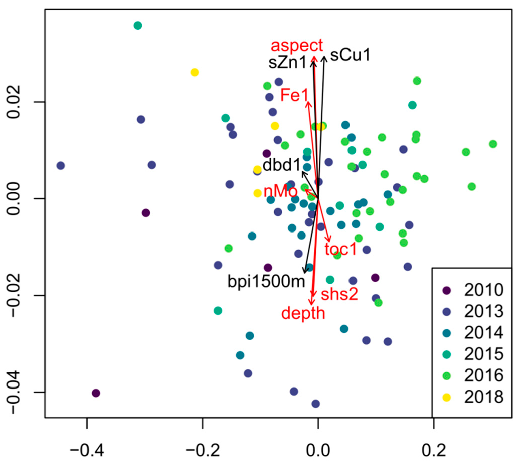
3.1. Spatial Prediction of Environmental Variables and Correlation with Meiofauna Patterns

Spatial predictions were computed for 53 sediment and 20 nodule characteristics. Only eleven of the sediment variable models explained more than zero per cent variance, whereas 15 nodule variables did (Table 1). All other variables were discarded as predictors for distribution modelling (see Table S1, Supplementary Materials).
Applying PERMANOVA to compare the community in different years, differences are highly significant (R: 0.22, p: 0.001). Pairwise comparison of the community observed in different years shows that there were significant differences in 2016 compared to all other years except for 2015 (Table 2). Further investigating the differences in dispersion between groups, variance between groups is slightly significant (F: 2.35, p: 0.047). Pairwise comparison of dispersion between groups shows that significant differences can be stated comparing 2014 to 2010, 2013 and 2015 (Table 2).
Despite significant differences between years, no distinct patterns can be observed visually across different sampling years investigating the meiofauna communities with Bray-Curtis Dissimilarity (Figure 2). Regarding correlations between meiofauna community patterns and the environmental variables, the bathymetric parameters water depth (p-value: 0.01) and aspect (p-value: 0.002) can be fitted highly significantly on the nMDS ordination. The direction of both vectors is roughly opposite (Figure 2). The vectors computed for the sediment parameters shear strength, measured in 2 cm sediment depth (p-value: 0.04), and total organic carbon, measured in 1 cm sediment depth (p-value: 0.04), both also highly significant, share direction with water depth (Figure 2). The content of iron in 1 cm sediment depth (p-value: 0.006), however, shares direction with the vector computed for aspect (Figure 2). The only highly significant vector derived from the nodule parameters is the content of molybdenum in the nodules (p-value: 0.03). The fitted vector is short and directed in a direction between the other vectors (Figure 2). Other, slightly less significant, vectors could be computed for the content of copper and zinc in 1 cm sediment depth (p-values: 0.05 and 0.07), the bathymetric position index at a scale of 1.5 km (p-value: 0.09) and dry bulk density also measured in 1 cm sediment depth.

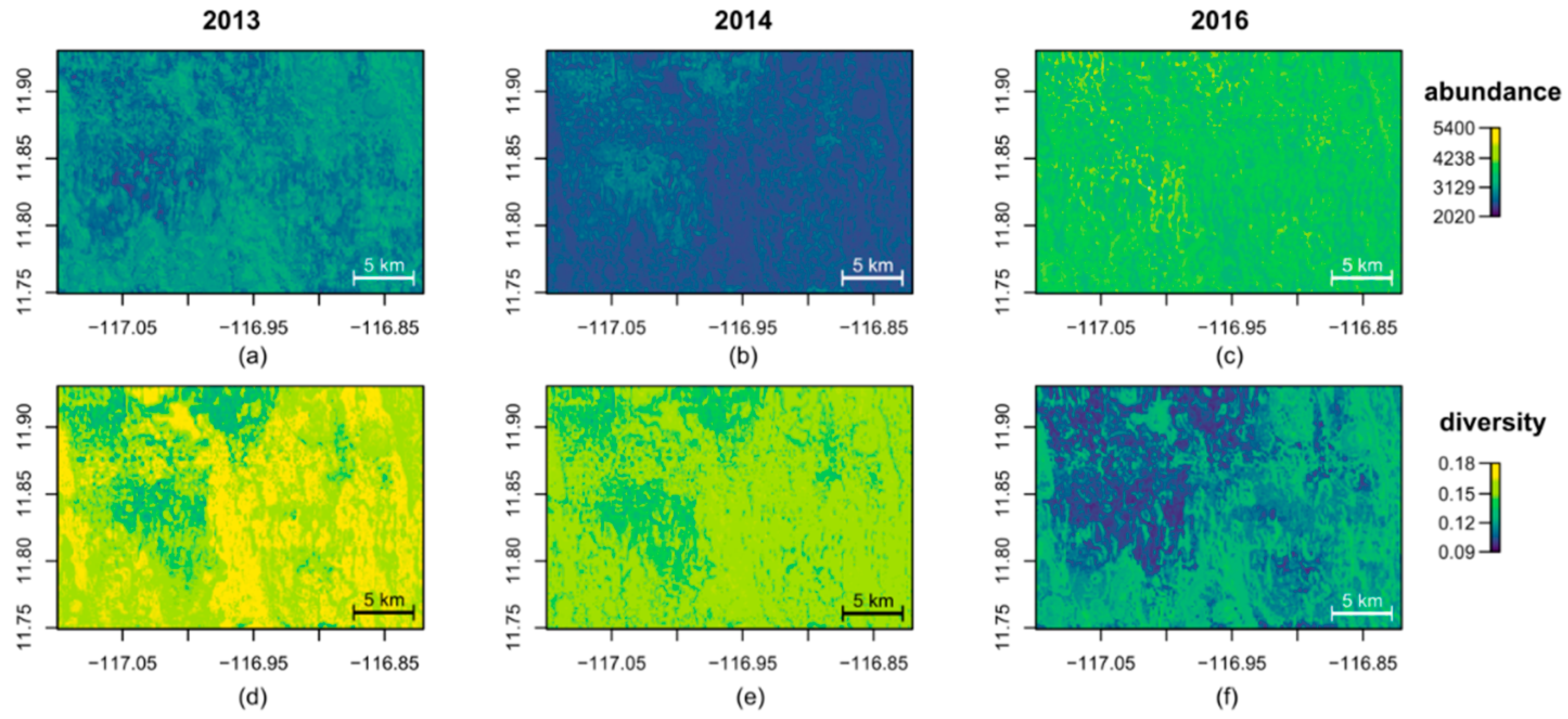
3.2. Spatial Prediction of Meiofauna Abundance and Diversity

Models computed with (a) bathymetry and backscatter predictors, (b) sediment and nodule predictors, or (c) all predictors together show almost identical performance (Table 3). Positively explained variance is obtained for the models on overall meiofauna abundance, taxon richness, diversity, evenness and abundance of the taxon Nematoda (Table 3). For all of these response variables, a significant, positive Pearson’s correlation can also be computed (Table 3). However, Pearson’s correlation is also significant for the taxa Annelida, Copepoda, Loricifera and Ostracoda (Table 3).
Overall meiofauna abundance is predicted to be slightly higher in elevated areas and reduced in areas with the highest backscatter (Figure 3a–c). Spatial patterns are almost identical comparing the predictions based on the model integrating all environmental variables to the predictions based also or solely on the modelled sediment and nodule characteristics, although correlation of predictions is lower comparing models integrating solely sediment and nodule variables to predictions based on variables derived from echosounder systems (Table 4). Higher meiofauna abundance is also distributed more evenly when modelling with sediment and nodule parameters in comparison to high peaks based on predictions solely integrating variables derived from echosounder systems (Figure 3a–c).
Simpson’s diversity is predicted to be highest in areas with low backscatter value (Figure 3d–f). Areas of predicted higher diversity include both elevations and depressions on the seafloor (Figure 3d–f). When computed solely with backscatter and bathymetry variables, patterns are identical but appear less distinct (Figure 3f). An intermediate smoothness can be observed when integrating all variables (Figure 3e). Correlation between predictions is high when they are produced with a subset of predictors or when using all available variables (Table 4).
Regarding the spatially predicted abundance of the taxon Nematoda, spatial patterns mirror the distribution of overall meiofauna abundance (Figure 3g–i). However, although the abundance of Nematoda is also distributed more evenly when modelled with sediment and nodule variables, the differences are less pronounced (Figure 3g–i). Correlation of predictions is almost identical to the correlations observed for the predictions of overall abundance (Table 4).

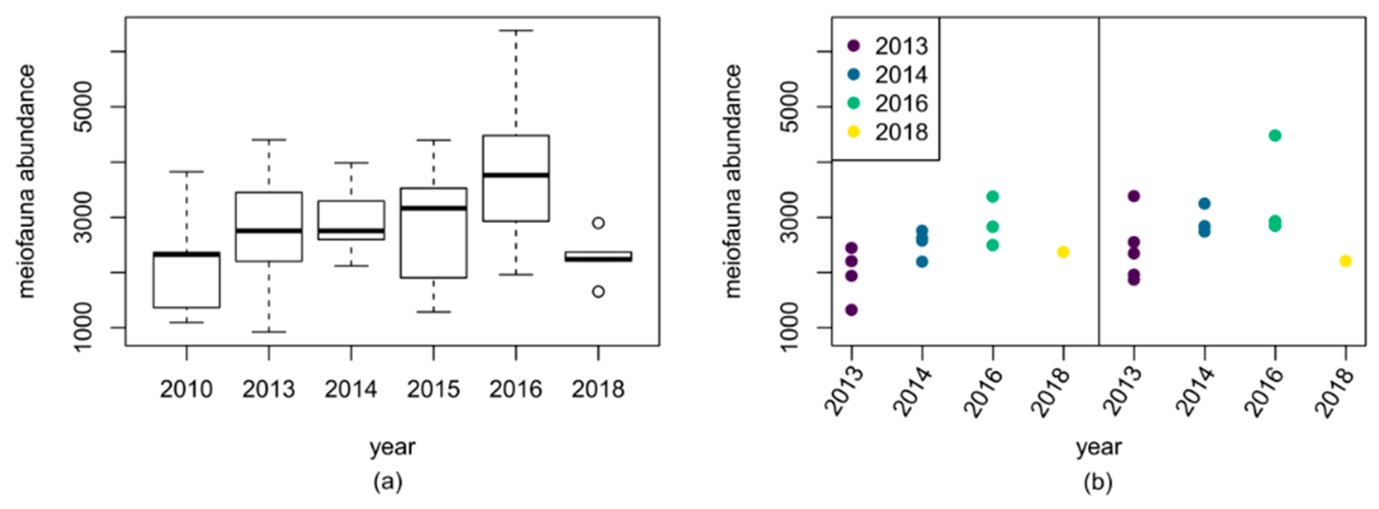
3.3. Differences in Meiofauna Abundance between Years

Regarding all years, mean abundance amounts to 3066 ± 994 individuals per 100 cm2 of sediment. Comparing trends between years shows that abundance has steadily increased from 2010, with a mean abundance of 2196 ± 1072 individuals per 100 cm2, to 2016, with 3806 ± 1044 individuals per 100 cm2. In 2018, abundance was again comparable to 2010, with a mean abundance of 2275 ± 444 individuals per 100 cm2 (Figure 4a).
Regarding only the two time series sites sampled during four years (magenta dots in Figure 1), an identical pattern can be observed. Overall abundance increases until 2016 but is low again in 2018; nevertheless, one core sample with very high abundance was also obtained in 2013, showing that variability between cores can be large (Figure 4b). However, only one core is available at each sampling site in 2018; hence, no statement can be given on variability in this year (Figure 4b).
Overall meiofauna abundance and diversity at high taxonomic level have been spatially predicted across the study area integrating meiofauna data solely obtained in 2013, 2014 and 2016. Model performance was worse compared to the random forest regressions using all available data as the response variable. Using data obtained in 2013, only the abundance of the taxa Annelida and Ostracoda could be modelled with explained variance higher than zero and a significant Pearson’s correlation (Table 5). The explained variance for evenness is slightly above zero (0.03), but here, Pearson’s correlation is not significant (Table 5). Although the number of available samples is lower in 2014 (Table 5), model performance is better using data obtained in that year. Explained variance is positive when modelling overall meiofauna abundance and taxon richness, as well as for the abundance of Nematoda, Loricifera and Tantulocarida (Table 5). Pearson’s correlation is significant for all of the predictions except for taxon richness (Table 5). In 2016, model performance is poor; the only decent model with explained variance above zero and a significant Pearson’s correlation was computed for Simpson’s Index of diversity (Table 5).
While in 2014 and 2016 the eastern part of the study area is predicted to have a comparably low abundance, it is elevated in this area in 2013 (Figure 5a–c). Comparing the predictions computed for abundance in the years 2014 and 2016, abundance is predicted to be lower in 2014 but expresses identical peaks in abundance in the western part of the study area (Figure 5b–c). In 2013, patterns are predicted slightly opposite to 2014 and 2016 (Figure 5a).
Comparing predicted abundances at all positions using Pearson’s correlation predictions based on samples obtained in 2014 and 2016 are positively correlated (Table 6). Correlating predictions of these two years with predictions based on samples from 2013, correlations are negative (Table 6). Spatial predictions of diversity are always positively correlated, although they are much higher when correlating 2013 and 2014 compared to correlations between those years and 2016 (Table 6).
Diversity is predicted to be generally lower in 2016 (Figure 5f). However, in 2016, spatial patterns are almost identical to spatial predictions computed with all available samples (Figure 5f). In 2014, the same pattern can be observed, although higher peaks in diversity occur in the west (Figure 5d). These spots of higher diversity are even more pronounced in 2013 (Figure 5e).

4. Discussion

Distribution modelling can be a powerful tool, not only for management issues [22], but also to investigate potential influences of environmental variables on organisms [23]. Hence, the spatial description of the abiotic environment is an important first step to investigate patterns affecting faunal distributions [28]. However, the only continuous and available layers with appropriate resolution were bathymetric variables and backscatter value; all of these variables were obtained as remote-sensing multibeam data. Continuous layers of relevant environmental variables such as grain size are scarcely available in the CCZ [13,24] or rather available on very low, global-scale resolution with information on, e.g., particulate organic matter [51], temperature, salinity or dissolved oxygen [52]. In this study, only 26 out of 73 parameters describing sediment and nodule characteristics proved to be significant and useful for modelling purposes. Hence, it is possible that some parameters display a distribution that is not mirrored in large-scale geographic features and also cannot be described using a combination of these.
Environmentally, the abyssal plain is a habitat characterized by low food flux and low physical energy [53] and, due to these conditions, the deep-sea fauna is usually highly diverse but occurs in low abundances [7]. Hence, the natural variability of the benthic fauna of all size classes is high on a small scale [8,54,55]. Therefore, if natural variability of environmental parameters as well as within the benthic fauna is too large, the model also cannot find patterns within the area. Regarding meiofauna, the variability between cores of the same multicorer deployment is often as large or even larger than the variability between cores of geographically separated deployments [56]. In our study, we could observe that such high variability can also be observed temporally, with heightened meiofauna abundance in only one core of the time series samples obtained in 2013.
Differences in predicted spatial distribution of meiofauna, however, are only minor, regardless of whether the model is computed based on bathymetry and backscatter, the predicted environmental parameters or all available variables. This might be due to the fact that the models predicting distribution of sediment and nodule characteristics use bathymetry and backscatter as predictor variables. Hence, significant influences of environmental variables on the community analysis based on Bray Curtis Dissimilarity largely mirror the influences of water depth and aspect. However, geographic features are known to mirror environmental drivers [23,57], and therefore, it is nonetheless useful to include predicted environmental layers to investigate their influences on the meiofauna. Most meiofauna variables have a smoother predicted distribution when integrating environmental parameters into the models. The use of higher resolution might actually not be useful for modelling the absolute values of meiofauna densities due to the high natural variability [13,56,58], which mainly allows for the prediction of trends. For computing predictions on species level, other taxa or other size classes, the additional use of environmental variables might become more important.
Water depth is often related to food availability, which usually decreases with increasing water depth [19,57,59]. In the study area, water depth varies only slightly between sampling positions, with the largest difference amounting to 80 m. However, despite similar directions of vectors across the meiofauna community depicted in Bray-Curtis Dissimilarity, Pearson’s correlation of −0.17 (p: ~0) between water depth and total organic carbon is even slightly negative in the study area, which may be the result of small-scale lateral transport of food particles. On a larger scale, there are distinct gradients in POC-flux across the CCZ [60] that are likely to influence meiofauna patterns across a distance of hundreds of kilometres [8]. These differences were found to even mask the small-scale influence of grain size on meiofauna [8]. On the small scale of this study, it is more likely that bottom currents influenced by topographic features such as seamounts and ridges as well as nodule sizes shape food availability and other sediment characteristics such as grain size [61,62,63]. Still, the variability of meiofauna sampled with the multicore might be influenced by variability on a smaller scale than that obtained with the larger boxcore samples and expressed in the predicted distribution of environmental variables.
The other continuously measured variable, backscatter value, is a proxy for the firmness of the seafloor and can therefore be used to predict the nodule cover on the soft-sedimented seafloor [9,64]. Different nodule patterns correlate with meiofauna in different ways. High nodule abundance can lead to lower meiofauna abundance simply by reducing the available sediment volume. However, communities in nodule areas also vary from communities observed in nodule-free areas [10,14], and in the Peru Basin, different communities have also been described from nodule crevices [16,17]. Nevertheless, it is unlikely that parameters such as the content of molybdenum or other elements in the nodules directly influence meiofauna patterns, as suggested by the community analysis (Figure 2). Most likely, they are either mirroring other features of the polymetallic nodules, e.g., porosity or size, or are proxies of other environmental variables that do influence the meiofauna community. Hence, they can be used as predictor variables for distribution modelling just as geographic features, although they possibly do not influence the meiofauna abundance directly.
In contrast, variation between models computed for the different years is high. Natural temporal variability of environmental conditions is high in the deep sea [5] and significant inter-annual differences have already been described for meiofauna in the French license area in the CCZ [11]. In this study, abundance of Nematoda was 1.5-fold higher in 2012 compared to abundance in 2004 [11], which is similar to the differences observed in this study, with a steady increase from 2010 to 2016, followed by a drop in abundance back to the level of 2010 in 2018. Spatially, a shift in abundance patterns seems to occur between 2013 and 2014 in our study area. A possible explanation could be shifts in the hydrodynamic regime of the study area due to changes in intertidal flow or benthic storms initiated by mesoscale eddies passing through the area [65]. Such events might influence meiofauna abundance within the sediment in different ways through, e.g., input and redistribution of food particles. At current velocities of 8 cm/s, resuspension of particles can be observed [63], which might limit the access of meiofauna to food particles deposited on the seafloor. However, model performance is weak if the models are solely based on data obtained in 2013, 2014 and 2016, and additionally, the number of samples available for 2010 and 2018 is too low for model computation. Therefore, it is difficult to clearly separate bias from natural patterns. Still, distribution models proved to be a useful tool to investigate temporal patterns in the spatial distribution of meiofauna abundance and diversity.
In the context of potential nodule mining, distribution models are an important tool to define appropriate protected areas and preservation zones within the CCZ and within individual contractor areas, respectively [13]. Here, we show that random forest regression can also help to investigate relationships between environmental variables and deep-sea meiofauna at the geographic scale of a potential mining operation even if these variables are obtained from different sampling sites. Although the variance explained by the models is rather low due to a small number of observations contrasting high variability, such models are the best possibility to investigate spatial distribution of the benthic fauna. Hence, the distribution modelling approach applied in this study could also prove useful for other size classes as well as on lower taxonomic levels, e.g., of the most abundant meiofauna taxon Nematoda. A potential issue might be the low dominance of species and genera in the deep sea [7], which can lead to few observations of the same taxon even within a distinctive sampling approach. However, the great differences between years also advocate for extended investigation of temporal variability to better define the levels of natural variability in order to obtain a better understanding of possible mining impacts and ecosystem recovery.
A similar modelling approach could be used to investigate the influence of pilot mining actions that do not only remove the sediment from the mining area but also provoke a sediment plume that will additionally affect more distant areas [5]. Although the specific effects of nodule mining in the deep sea are uncertain, impacts are likely to be severe [5]. Combining distribution models of benthic organisms with models of the impact, e.g., of the sediment plume [63], could help in the establishment of preservation zones that are out of the impact area of the disturbance. Furthermore, distribution models can help to estimate possible spatial extents of the impact during monitoring and later to investigate recovery of the disturbed areas.

Supplementary Materials

The following are available online at https://www.mdpi.com/1424-2818/13/1/3/s1. Table S1: Model evaluations of the random forest regressions computed for the sediment and nodule characteristics not used for distribution modelling of meiofauna according to the percentage of explained variance and Pearson’s correlation (* indicating significance). The number of observations that could be integrated into the model is given. Elements refer to their concentration in the sediment and the nodules, respectively. Centimetres refer to the sampling depth in the sediment. Table S2: Meiofauna abundance converted to 100 cm2 obtained in the study area; the multicore from BGR (Federal Institute for Geosciences and Mineral Resources) is equipped with eight cores with the diameter of 7.4 cm, the multicore from DZMB (German Centre for Marine Biodiversity Research) is equipped with 12 cores with a diameter of 9.6 cm.

Author Contributions

Conceptualization, K.U. and P.M.A.; methodology, K.U. and P.M.A.; software, K.U.; validation, K.U. and P.M.A.; formal analysis, K.U.; investigation, all authors; resources, A.V., T.K. and P.M.A.; data curation, K.U. and A.V.; writing—original draft preparation, K.U.; writing—review and editing, all authors; visualization, K.U.; supervision, P.M.A.; project administration, P.M.A.; funding acquisition, P.M.A. All authors have read and agreed to the published version of the manuscript.

Funding

This research was funded by the German Federal Ministry of Education and Research (BMBF), grant numbers 03F0707E and 03F0812E, as a contribution to the European project JPI-Oceans “Ecological Aspects of Deep-Sea Mining”. The APC is funded via the Open Access Publication Fund of the Carl von Ossietzky University Oldenburg.

Data Availability Statement

Data on meiofauna abundance from the years 2010 to 2016 are a subset of the meiofauna dataset used in a previous study [13] and are already deposited in the PANGAEA data publisher and information system (https://doi.org/10.1594/PANGAEA.912217). The data used in this study, as well as additional data on meiofauna abundance obtained in 2018, can be found in Table S2 (Supplementary Materials). Distribution maps of meiofauna will be deposited in the PANGAEA data publisher and information system. The environmental data presented in this study are available on request from BGR with the exception of confidential data associated with the nodule resource ([email protected]).

Acknowledgments

We thank the captains and crew of the research vessels “Sonne”, “Kilo Moana” and “L’Atalante” for their help and expertise during the scientific cruises “Mangan2008”, “Mangan2010 (SO-205)”, “BIONOD2012”, “Mangan2013”, “Mangan2014”, “FLUM (SO-240)”, “EcoResponse (SO-239)”, “Mangan2016” and “Mangan2018 (SO-262). We especially thank Lena Albers, Annika Janssen, Sarah Menke, Marco Bruhn, Annika Hellmann and Focke Weerts for their help with processing and sorting of the meiofauna.

Conflicts of Interest

The authors declare no conflict of interest. The funders had no role in the design of the study; in the collection, analyses, or interpretation of data; in the writing of the manuscript, or in the decision to publish the results.

References

  1. Wedding, L.M.; Reiter, S.M.; Smith, C.R.; Gjerde, K.M.; Kittinger, J.N.; Friedlander, A.M.; Gaines, S.D.; Clark, M.R.; Thurnherr, A.M.; Hardy, S.M.; et al. Managing mining of the deep seabed. Science 2015, 349, 144–145. [Google Scholar] [CrossRef] [PubMed] [Green Version]
  2. Kuhn, T.; Wegorzewski, A.; Rühlemann, C.; Vink, A. Composition, formation, and occurrence of polymetallic nodules. In Deep-Sea Mining: Resource Potential, Technical and Environmental Considerations; Sharma, R., Ed.; Springer: Cham, Switzerland, 2017; pp. 23–63. ISBN 978-3-319-52557-0. [Google Scholar] [CrossRef]
  3. Cuvelier, D.; Gollner, S.; Jones, D.O.B.; Kaiser, S.; Martínez Arbizu, P.; Menzel, L.; Mestre, N.C.; Morato, T.; Pham, C.; Pradillon, F.; et al. Potential Mitigation and Restoration Actions in Ecosystems Impacted by Seabed Mining. Front. Mar. Sci. 2018, 5. [Google Scholar] [CrossRef] [Green Version]
  4. Gollner, S.; Kaiser, S.; Menzel, L.; Jones, D.O.B.; Brown, A.; Mestre, N.C.; van Oevelen, D.; Menot, L.; Colaço, A.; Canals, M.; et al. Resilience of benthic deep-sea fauna to mining activities. Mar. Environ. Res. 2017, 129, 76–101. [Google Scholar] [CrossRef] [PubMed] [Green Version]
  5. Jones, D.O.B.; Kaiser, S.; Sweetman, A.K.; Smith, C.R.; Menot, L.; Vink, A.; Trueblood, D.; Greinert, J.; Billett, D.S.M.; Martínez Arbizu, P.; et al. Biological responses to disturbance from simulated deep-sea polymetallic nodule mining. PLoS ONE 2017, 12, e0171750. [Google Scholar] [CrossRef]
  6. Kaiser, S.; Smith, C.R.; Martínez Arbizu, P. Editorial: Biodiversity of the Clarion Clipperton Fracture Zone. Mar. Biodivers. 2017, 47, 259–264. [Google Scholar] [CrossRef]
  7. Ramirez-Llodra, E.; Brandt, A.; Danovaro, R.; De Mol, B.; Escobar, E.; German, C.R.; Levin, L.A.; Martínez Arbizu, P.; Menot, L.; Buhl-Mortensen, P.; et al. Deep, diverse and definitely different: Unique attributes of the world’s largest ecosystem. Biogeosciences 2010, 7, 2851–2899. [Google Scholar] [CrossRef] [Green Version]
  8. Hauquier, F.; Macheriotou, L.; Bezerra, T.N.; Egho, G.; Martínez Arbizu, P.; Vanreusel, A. Distribution of free-living marine nematodes in the Clarion–Clipperton Zone: Implications for future deep-sea mining scenarios. Biogeosciences 2019, 16, 3475–3489. [Google Scholar] [CrossRef] [Green Version]
  9. Kuhn, T.; Uhlenkott, K.; Vink, A.; Rühlemann, C.; Martínez Arbizu, P. Manganese nodule fields from the Northeast Pacific as benthic habitats. In Seafloor Geomorphology as Benthic Habitat: GeoHab Atlas of Seafloor Geomorphic Features and Benthic Habitats; Harris, P.T., Baker, E., Eds.; Elsevier: Amsterdam, The Netherlands, 2020; pp. 933–947. ISBN 978-0-12-814960-7. [Google Scholar]
  10. Miljutina, M.A.; Miljutin, D.M.; Mahatma, R.; Galéron, J. Deep-sea nematode assemblages of the Clarion-Clipperton Nodule Province (Tropical North-Eastern Pacific). Mar. Biodivers. 2010, 40, 1–15. [Google Scholar] [CrossRef]
  11. Miljutin, D.; Miljutina, M.; Messié, M. Changes in abundance and community structure of nematodes from the abyssal polymetallic nodule field, Tropical Northeast Pacific. Deep Sea Res. Part Oceanogr. Res. Pap. 2015, 106, 126–135. [Google Scholar] [CrossRef]
  12. Pape, E.; Bezerra, T.N.; Hauquier, F.; Vanreusel, A. Limited spatial and temporal variability in meiofauna and nematode communities at distant but environmentally similar sites in an area of interest for deep-sea mining. Front. Mar. Sci. 2017, 4. [Google Scholar] [CrossRef]
  13. Uhlenkott, K.; Vink, A.; Kuhn, T.; Martínez Arbizu, P. Predicting meiofauna abundance to define preservation and impact zones in a deep-sea mining context using random forest modelling. J. Appl. Ecol. 2020, 57, 1210–1221. [Google Scholar] [CrossRef]
  14. Singh, R.; Miljutin, D.M.; Vanreusel, A.; Radziejewska, T.; Miljutina, M.M.; Tchesunov, A.; Bussau, C.; Galtsova, V.; Martínez Arbizu, P. Nematode communities inhabiting the soft deep-sea sediment in polymetallic nodule fields: Do they differ from those in the nodule-free abyssal areas? Mar. Biol. Res. 2016, 12, 345–359. [Google Scholar] [CrossRef]
  15. Vanreusel, A.; Fonseca, G.; Danovaro, R.; Silva, M.C.D.; Esteves, A.M.; Ferrero, T.; Gad, G.; Galtsova, V.; Gambi, C.; da Fonsêca Genevois, V.; et al. The contribution of deep-sea macrohabitat heterogeneity to global nematode diversity. Mar. Ecol. 2010, 31, 6–20. [Google Scholar] [CrossRef] [Green Version]
  16. Thiel, H.; Schriever, G.; Bussau, C.; Borowski, C. Manganese nodule crevice fauna. Deep Sea Res. Part Oceanogr. Res. Pap. 1993, 40, 419–423. [Google Scholar] [CrossRef]
  17. Bussau, C.; Schriever, G.; Thiel, H. Evaluation of abyssal metazoan meiofauna from a manganese nodule area of the Eastern South Pacific. Vie Milieu 1995, 45, 39–48. [Google Scholar]
  18. Schratzberger, M.; Larcombe, P. The role of the sedimentary regime in shaping the distribution of subtidal sandbank environments and the associated meiofaunal nematode communities: An example from the Southern North Sea. PLoS ONE 2014, 9, e109445. [Google Scholar] [CrossRef]
  19. Danovaro, R.; Gambi, C.; Della Croce, N. Meiofauna hotspot in the Atacama Trench, eastern South Pacific Ocean. Deep-Sea Res. Part I 2002, 49, 843–857. [Google Scholar] [CrossRef]
  20. Guidi-Guilvard, L.D.; Thistle, D.; Khripounoff, A.; Gasparini, S. Dynamics of benthic copepods and other meiofauna in the benthic boundary layer of the deep NW Mediterranean Sea. Mar. Ecol. Prog. Ser. 2009, 396, 181–195. [Google Scholar] [CrossRef]
  21. Zeppilli, D.; Pusceddu, A.; Trincardi, F.; Danovaro, R. Seafloor heterogeneity influences the biodiversity–ecosystem functioning relationships in the deep sea. Sci. Rep. 2016, 6, 1–12. [Google Scholar] [CrossRef] [Green Version]
  22. Guisan, A.; Thuiller, W. Predicting species distribution: Offering more than simple habitat models. Ecol. Lett. 2005, 8, 993–1009. [Google Scholar] [CrossRef]
  23. Elith, J.; Leathwick, J.R. Species distribution models: Ecological explanation and prediction across space and time. Annu. Rev. Ecol. Evol. Syst. 2009, 40, 677–697. [Google Scholar] [CrossRef]
  24. Wedding, L.M.; Friedlander, A.M.; Kittinger, J.N.; Watling, L.; Gaines, S.D.; Bennett, M.; Hardy, S.M.; Smith, C.R. From principles to practice: A spatial approach to systematic conservation planning in the deep sea. Proc. R. Soc. B Biol. Sci. 2013, 280, 20131684. [Google Scholar] [CrossRef] [PubMed] [Green Version]
  25. Warton, D.I.; Shipley, B.; Hastie, T. CATS regression—A model-based approach to studying trait-based community assembly. Methods Ecol. Evol. 2015, 6, 389–398. [Google Scholar] [CrossRef]
  26. Breiman, L. Random forests. Mach. Learn. 2001, 45, 5–32. [Google Scholar] [CrossRef] [Green Version]
  27. Hastie, T.; Tibshirani, R.; Friedman, J.H. The Elements of Statistical Learning: Data Mining, Inference and Prediction, 2nd ed.; Springer Science & Business Media: New York, NY, USA, 2009; ISBN 978-0-387-95284-0. [Google Scholar]
  28. Ostmann, A.; Schnurr, S.; Martínez Arbizu, P. Marine environment around Iceland: Hydrography, sediments and first predictive models of Icelandic deep-sea sediment characteristics. Pol. Polar Res. 2014, 35, 151–176. [Google Scholar] [CrossRef]
  29. Rühlemann, C. Shipboard Scientific Party. In MANGAN 2013; Bundesanstalt für Geowissenschaften und Rohstoffe (BGR): Hannover, Germany, 2014. [Google Scholar]
  30. Rühlemann, C. Shipboard Scientific Party. In MANGAN 2014; Bundesanstalt für Geowissenschaften und Rohstoffe (BGR): Hannover, Germany, 2015. [Google Scholar]
  31. Rühlemann, C. Shipboard Scientific Party. In MANGAN 2016; Bundesanstalt für Geowissenschaften und Rohstoffe (BGR): Hannover, Germany, 2017. [Google Scholar]
  32. Rühlemann, C. Shipboard Scientific Party. In MANGAN 2018; Bundesanstalt für Geowissenschaften und Rohstoffe (BGR): Hannover, Germany, 2019. [Google Scholar]
  33. Rühlemann, C. Shipboard Scientific Party. In SO205 MANGAN; Bundesanstalt für Geowissenschaften und Rohstoffe (BGR): Hannover, Germany, 2010. [Google Scholar]
  34. Martínez Arbizu, P. Shipboard Scientific Party. In SO239 EcoResponse: Assessing the Ecology, Connectivity and Resilience of Polymetallic Nodule Field Systems; GEOMAR Helmholtz-Zentrum für Ozeanforschung: Kiel, Germany, 2015. [Google Scholar]
  35. Heip, C.; Vincx, M.; Vranken, G. The ecology of marine nematodes. Oceanogr. Mar. Biol. Annu. Rev. 1985, 23, 399–489. [Google Scholar]
  36. Simpson, E.H. Measurement of Diversity. Nature 1949, 163, 688. [Google Scholar] [CrossRef]
  37. Pielou, E.C. The measurement of diversity in different types of biological collections. J. Theor. Biol. 1966, 13, 131–144. [Google Scholar] [CrossRef]
  38. Wiedicke-Hombach, M. Shipboard Scientific Party. In Campaign “MANGAN 2008” with R/V Kilo Moana; Bundesanstalt für Geowissenschaften und Rohstoffe (BGR): Hannover, Germany, 2009. [Google Scholar]
  39. Rühlemann, C. Shipboard Scientific Party. In BIONOD Volume 1: German License Area; Bundesanstalt für Geowissenschaften und Rohstoffe (BGR): Hannover, Germany, 2012. [Google Scholar]
  40. Kuhn, T. Shipboard Scientific Party. In SO240 FLUM: Low-Temperature Fluid Circulation at Seamounts and Hydrothermal Pits: Heat Flow Regime, Impact on Biogeochemical Processes, and Its Potential Influence on the Occurrence and Composition of Manganese Nodules in the Equatorial Eastern Pacific; Bundesanstalt für Geowissenschaften und Rohstoffe (BGR): Hannover, Germany, 2015. [Google Scholar]
  41. Hijmans, R.J. Raster: Geographic Data Analysis and Modeling; The Comprehensive R Archive Network: Vienna, Austria, 2020. [Google Scholar]
  42. Liaw, A.; Wiener, M. Classification and regression by randomForest. R News 2002, 2, 18–22. [Google Scholar]
  43. Bray, J.R.; Curtis, J.T. An Ordination of the Upland Forest Communities of Southern Wisconsin. Ecol. Monogr. 1957, 27, 325–349. [Google Scholar] [CrossRef]
  44. Oksanen, J.; Blanchet, F.G.; Friendly, M.; Kindt, R.; Legendre, P.; McGlinn, D.; Minchin, P.R.; O’Hara, R.B.; Simpson, G.L.; Solymos, P.; et al. Vegan: Community Ecology Package; The Comprehensive R Archive Network: Vienna, Austria, 2019. [Google Scholar]
  45. Anderson, M.J. A new method for non-parametric multivariate analysis of variance. Austral. Ecol. 2001, 26, 32–46. [Google Scholar] [CrossRef]
  46. Martinez Arbizu, P. pairwiseAdonis: Pairwise Multilevel Comparison Using Adonis; The Comprehensive R Archive Network: Vienna, Austria, 2019. [Google Scholar]
  47. R Core Team. R: A Language and Environment for Statistical Computing; R Foundation for Statistical Computing: Vienna, Austria, 2019. [Google Scholar]
  48. Keitt, T. colorRamps: Builds Color Tables; The Comprehensive R Archive Network: Vienna, Austria, 2012. [Google Scholar]
  49. Rabosky, A.R.D.; Cox, C.L.; Rabosky, D.L.; Title, P.O.; Holmes, I.A.; Feldman, A.; McGuire, J.A. Coral snakes predict the evolution of mimicry across New World snakes. Nat. Commun. 2016, 7, 1–9. [Google Scholar] [CrossRef]
  50. Garnier, S. viridisLite: Default Color Maps from “matplotlib” (Lite Version); The Comprehensive R Archive Network: Vienna, Austria, 2018. [Google Scholar]
  51. Lutz, M.J.; Caldeira, K.; Dunbar, R.B.; Behrenfeld, M.J. Seasonal rhythms of net primary production and particulate organic carbon flux to depth describe the efficiency of biological pump in the global ocean. J. Geophys. Res. Oceans 2007, 112. [Google Scholar] [CrossRef]
  52. Sayre, R.G.; Wright, D.J.; Breyer, S.P.; Butler, K.A.; Van Graafeiland, K.; Costello, M.J.; Harris, P.T.; Goodin, K.L.; Guinotte, J.M.; Basher, Z.; et al. A three-dimensional mapping of the ocean based on environmental data. Oceanography 2017, 30, 90–103. [Google Scholar] [CrossRef]
  53. Glover, A.G.; Smith, C.R. The deep-sea floor ecosystem: Current status and prospects of anthropogenic change by the year 2025. Environ. Conserv. 2003, 30, 219–241. [Google Scholar] [CrossRef] [Green Version]
  54. Janssen, A.; Kaiser, S.; Meißner, K.; Brenke, N.; Menot, L.; Martínez Arbizu, P. A reverse taxonomic approach to assess macrofaunal distribution patterns in abyssal Pacific polymetallic nodule fields. PLoS ONE 2015, 10, e0117790. [Google Scholar] [CrossRef] [Green Version]
  55. Simon-Lledó, E.; Pomee, C.; Ahokava, A.; Drazen, J.C.; Leitner, A.B.; Flynn, A.; Jones, D.O.B. Multi-scale variations in invertebrate and fish megafauna in the mid-eastern Clarion Clipperton Zone. Prog. Oceanogr. 2020, 187, 102405. [Google Scholar] [CrossRef]
  56. Rosli, N.; Leduc, D.; Rowden, A.A.; Probert, P.K. Review of recent trends in ecological studies of deep-sea meiofauna, with focus on patterns and processes at small to regional spatial scales. Mar. Biodivers. 2018, 48, 13–34. [Google Scholar] [CrossRef]
  57. Ostmann, A.; Martínez Arbizu, P. Predictive models using randomForest regression for distribution patterns of meiofauna in Icelandic waters. Mar. Biodivers. 2018, 48, 719–735. [Google Scholar] [CrossRef]
  58. Lambshead, P.J.D.; Brown, C.J.; Ferrero, T.J.; Hawkins, L.E.; Smith, C.R.; Mitchell, N.J. Biodiversity of nematode assemblages from the region of the Clarion-Clipperton Fracture Zone, an area of commercial mining interest. BMC Ecol. 2003, 12, 1. [Google Scholar] [CrossRef]
  59. Gambi, C.; Lampadariou, N.; Danovaro, R. Latitudinal, longitudinal and bathymetric patterns of abundance, biomass of metazoan meiofauna: Importance of the rare taxa and anomalies in the deep Mediterranean Sea. Adv. Oceanogr. Limnol. 2010, 1, 167–197. [Google Scholar] [CrossRef]
  60. Volz, J.B.; Mogollón, J.M.; Geibert, W.; Arbizu, P.M.; Koschinsky, A.; Kasten, S. Natural spatial variability of depositional conditions, biogeochemical processes and element fluxes in sediments of the eastern Clarion-Clipperton Zone, Pacific Ocean. Deep Sea Res. Part. Oceanogr. Res. Pap. 2018, 140, 159–172. [Google Scholar] [CrossRef]
  61. Rogers, A.D. The biology of seamounts. In Advances in Marine Biology; Elsevier: Amsterdam, The Netherlands, 1994; Volume 30, pp. 305–350. ISBN 978-0-12-026130-7. [Google Scholar] [CrossRef]
  62. Stefanoudis, P.V.; Bett, B.J.; Gooday, A.J. Abyssal hills: Influence of topography on benthic foraminiferal assemblages. Prog. Oceanogr. 2016, 148, 44–55. [Google Scholar] [CrossRef] [Green Version]
  63. Gillard, B.; Purkiani, K.; Chatzievangelou, D.; Vink, A.; Iversen, M.H.; Thomsen, L. Physical and hydrodynamic properties of deep sea mining-generated, abyssal sediment plumes in the Clarion Clipperton Fracture Zone (eastern-central Pacific). Elem. Sci Anthr. 2019, 7, 5. [Google Scholar] [CrossRef] [Green Version]
  64. Knobloch, A.; Kuhn, T.; Rühlemann, C.; Hertwig, T.; Zeissler, K.-O.; Noack, S. Predictive mapping of the nodule abundance and mineral resource estimation in the Clarion-Clipperton Zone using artificial neural networks and classical geostatistical methods. In Deep-Sea Mining: Resource Potential, Technical and Environmental Considerations; Sharma, R., Ed.; Springer: Cham, Switzerland, 2017; pp. 189–212. ISBN 978-3-319-52557-0. [Google Scholar] [CrossRef]
  65. Aleynik, D.; Inall, M.E.; Dale, A.; Vink, A. Impact of remotely generated eddies on plume dispersion at abyssal mining sites in the Pacific. Sci. Rep. 2017, 7, 1–14. [Google Scholar] [CrossRef] [Green Version]
Figure 1. Bathymetric map of the German license area for the exploration of polymetallic nodules with the study area (magenta square) located in the eastern part of the area; points indicate sampling positions of boxcorer deployments (bottom left) and detailed bathymetric map of the study area; points indicate sampling positions of multicorer deployments (top right). Two time-series stations that were sampled in four different years (2013, 2014, 2016 and 2018) are marked in magenta.
Diversity 13 00003 g001
Figure 2. Non-metric multidimensional scaling of the Bray-Curtis Dissimilarity (stress: 0.02) computed for the meiofauna community on high taxonomic level regarding each core as one individual sample. The colours of the points indicate the year of sampling. Vectors correlate environmental variables to the community patterns; red arrows indicate high significance of the vector; black arrows indicate low significance. aspect: cardinal direction of the slope, BPI1500m: bathymetric position index across a radius of 1.5 km, dbd4: dry bulk density in 4 cm sediment depth, depth: water depth, nMo: content of molybdenum in polymetallic nodules, sCu1: content of copper in 1 cm sediment depth, sFe1: content of iron in 1 cm sediment depth, sZn1: content of zinc in 1 cm sediment depth, shs2: shear strength in 2 cm sediment depth, toc1: total organic carbon in 1 cm sediment depth.
Diversity 13 00003 g002
Figure 3. Distribution maps based on random forest regression using backscatter and bathymetry only (left), all available predictors (middle) and sediment and nodule parameters only (right) as predictor variables. Maps show overall meiofauna abundance (ac), Simpson’s Index on high taxonomic level (df) and abundance of Nematoda (gi).
Diversity 13 00003 g003
Figure 4. Boxplot of overall meiofauna abundance per 100 cm2 of sediment in different years, with the middle line being the median, the box referring to the first and third quartile and the whiskers indicating maxima and minima within a 1.5-fold interquartile range; potential outliers are indicated by points (a); overall abundance of meiofauna per 100 cm2 in samples obtained in consecutive years from the two time-series sample sites (see magenta dots in Figure 1: left: northwestern station; right: southeastern station) (b).
Diversity 13 00003 g004
Figure 5. Distribution maps based on random forest regression of overall meiofauna abundance (ac) and Simpson’s Index of diversity at a high taxonomic level (df) based only on response data obtained in 2013, 2014 and 2016 using backscatter, bathymetry, sediment and nodule parameters as predictor variables.
Diversity 13 00003 g005
Table 1. Model evaluations of the random forest regressions computed for the sediment and nodule characteristics used for distribution modelling of meiofauna according to the percentage of explained variance and Pearson’s correlation (* indicating significance). The number of observations that could be integrated into the model is given. Elements refer to their concentration in the sediment and the nodules, respectively. Centimetres refer to the sampling depth in the sediment.
Variable% Explained VariancePearson’s CorrelationNumber of Observations
sediment parameters
iron (1 cm)0.000.1630
copper (1 cm)0.040.2230
zinc (1 cm)0.030.2330
dry bulk density (1 cm)0.020.23 *133
dry bulk density (4 cm)0.170.42 *133
shear strength (2 cm)0.030.2 *133
total organic carbon (1cm)0.050.26 *114
total inorganic carbon (1 cm)0.230.48 *114
total carbon (1 cm)0.250.51 *114
total inorganic carbon (4 cm)0.230.48 *114
total carbon (4 cm)0.230.49 *114
nodule parameters
wet weight nodules0.440.66 *211
mean size nodules 0.370.6 *211
ratio large (>4 cm) to small (<4 cm) nodules0.080.31 *211
number of nodules0.380.62 *211
cobalt0.080.33 *211
iron0.170.41 *211
nickel0.130.37 *211
zinc0.110.36 *211
lithium0.150.39 *211
titanium0.030.24 *211
zirconium0.230.48 *211
molybdenum0.20.44 *211
barium0.20.45 *211
quotient of manganese and iron0.090.32 *211
sum of rare earth elements0.140.37 *211
Table 2. Pairwise permutational analysis of variance (PERMANOVA, pairwise.adonis) to compare the meiofauna community observed in different years, p-value adjusted according to the Bonferroni correction, and significance of pairwise comparison of group dispersion (permutest.betadisper) (* indicating significance).
pairwise.adonispermutest.betadisper
PairF-ModelR2adj. p-Valuep-Value
2013 vs. 20102.500.0610.60
2013 vs. 20141.070.0210.003 *
2013 vs. 20150.300.0110.97
2013 vs. 201614.020.190.02 *0.26
2013 vs. 20181.180.0310.09
2010 vs. 20147.930.230.050.02 *
2010 vs. 20151.990.1310.69
2010 vs. 201613.650.290.02 *0.25
2010 vs. 20180.680.0810.23
2014 vs. 20150.660.0210.05 *
2014 vs. 201613.470.210.03 *0.06
2014 vs. 20186.300.20.260.71
2015 vs. 20165.240.120.290.45
2015 vs. 20181.420.110.25
2016 vs. 201812.760.280.03 *0.22
Table 3. Model evaluations of the random forest regressions computed for overall meiofauna abundance, taxon richness and diversity as well as different higher meiofauna taxa according to the percentage of explained variance and Pearson’s correlation using backscatter and bathymetry only (a), sediment and nodule parameters only (b) or all available predictors (c) as predictor variables. (* indicates significance < 0.05).
abc
Variable% Explained VariancePearson’s Correlation% Explained VariancePearson’s Correlation% Explained VariancePearson’s Correlation
overall abundance0.100.45 *0.150.43 *0.160.45 *
taxon richness0.190.47 *0.190.48 *0.190.48 *
Simpson’s Index0.140.39 *0.150.44 *0.140.43 *
evenness0.140.44 *0.150.45 *0.150.44 *
Annelida−0.030.24 *−0.040.23 *−0.050.23 *
Copepoda−0.020.24 *−0.030.24 *−0.050.22 *
Gastrotricha−0.150.11−0.160.011−0.160.01
Kinoryncha−0.25−0.03−0.26−0.03−0.28−0.03
Loricifera−0.030.27 *−0.100.23 *0.080.25 *
Nematoda0.180.46 *0.160.45 *0.170.46 *
Ostracoda−0.040.26 *−0.050.26 *−0.050.25 *
Tantulocarida−0.100.09−0.100.09−0.110.08
Tardigrada−0.31−0.12−0.36−0.15−0.33−0.14
Table 4. Pairwise Pearson’s correlation of the spatial predictions based on random forest regression computed for overall meiofauna abundance, Simpson’s diversity index and abundance of the taxon Nematoda using backscatter and bathymetry only (a), sediment and nodule parameters only (b) or all available predictors (c) as predictor variables. All correlations are highly significant.
Variablea vs. cb vs. ca vs. b
overall abundance0.850.780.42
Simpson’s Index0.810.910.60
Nematoda abundance0.830.810.42
Table 5. Model evaluations of the random forest regressions computed for overall meiofauna abundance, taxon richness and diversity, as well as different higher meiofauna taxa, integrating only data obtained in 2013, 2014 and 2016 according to the percentage of explained variance and Pearson’s correlation (* indicating significance).
Variable201320142016
% Explained VariancePearson’s CorrelationNumber of Observations% Explained VariancePearson’s CorrelationNumber of Observations% Explained VariancePearson’s CorrelationNumber of Observations
overall abundance−0.030.27330.230.53 *23−0.110.2330
taxon richness−0.020.29330.070.4023−0.110.2530
Simpson’s Index−0.030.2933−0.200.15230.090.41 *30
evenness0.030.36 *33−0.070.2723−0.100.2530
Annelida0.220.51 *33−0.290.0223−0.040.3030
Copepoda−0.020.2933−0.47−0.1023−0.190.1730
Gastrotricha−0.41−0.1233−0.53−0.2423−0.060.2930
Kinoryncha−0.36−0.1333−0.32−0.0023−0.49−0.1530
Loricifera−0.070.26330.310.58 *23−0.57−0.1930
Nematoda−0.040.27330.220.53 *23−0.060.2730
Ostracoda0.160.46 *33−0.40−0.1723−0.410.0330
Tantulocarida−0.27−0.09330.150.46 *23−0.51−0.1830
Tardigrada−0.35−0.2433−0.30−0.0023−0.66−0.37 *30
Table 6. Pairwise Pearson’s correlation between spatial prediction of overall meiofauna abundance (upper, right-hand triangle) and meiofauna diversity on high taxonomic level (Simpson’s Index) (lower, left-hand triangle) including only response variables obtained in one year; all values are highly significant.
Year201320142016
2013-−0.39−0.12
20140.87-0.37
20160.650.59-
Publisher’s Note: MDPI stays neutral with regard to jurisdictional claims in published maps and institutional affiliations.

