Abstract
Although DNA barcodes-based operational taxonomic units (OTUs) are increasingly used in earthworm research, the relative efficiency of the different methods available to delimit them has not yet been tested on a comprehensive dataset. For this study, we used three datasets containing 651, 2304 and 4773 COI barcodes of earthworms from French Guiana, respectively, to compare five of these methods: two phylogenetic methods—namely Poisson Tree Processes (PTP) and General Mixed Yule Coalescence (GMYC)—and three distance matrix methods—namely Refined Single Linkage (RESL, used for assigning Barcode Index Numbers in the Barcode of Life Data systems), Automatic Barcode Gap Discovery (ABGD), and Assemble Species by Automatic Partitioning (ASAP). We found that phylogenetic approaches are less suitable for delineating OTUs from DNA barcodes in earthworms, especially for large sets of sequences. The computation times are unreasonable, they often fail to converge, and they also show a strong tendency to oversplit species. Among distance-based methods, RESL also has a clear tendency to oversplitting, while ABGD and ASAP are less prone to mismatches and have short computation times. ASAP requires less a priori knowledge for model parameterisation than AGBD, provides efficient graphical outputs, and has a much lower tendency to generate mismatches.
1. Introduction
Molecular approaches are increasingly used in the field of biodiversity sciences. In earthworm studies, DNA-based approaches have led to particularly significant advances in the fields of evolution and ecology [1]. The barcode region of the mitochondrial gene cytochrome c oxidase (COI) [2] is increasingly used to overcome the limitations of morphology-based identification [3]. Indeed, species discrimination by morphology often relies on the examination of discrete characters or is simply impossible in the case of cryptic species. In most cases, juveniles also lack the diagnostic characters necessary for species identification, even though they often represent more than 50–60% of the sampled individuals. Therefore, the use of DNA barcoding represents a good alternative to overcome these difficulties. DNA barcodes can be used to delineate Operational Taxonomic Units (OTUs), which are increasingly used to support integrative taxonomy approaches, or in ecology, where they can be used as species proxies to estimate community diversity and describe their spatial distribution [3,4,5].
Different methods based on single-locus data are available to delineate OTUs in DNA barcode data. These methods can be classified into two main families, which differ in the bioinformatics approach used. Some methods such as the General Mixed Yule-Coalescent model (GMYC) [6], or the Poisson Tree Process model (PTP) [7], use previously constructed phylogenetic trees. Other methods are based on the analysis of distance matrices of nucleotide sequences. This last category includes the Refined Single Linkage Algorithm (RESL) [8], Automatic Barcode Gap Discovery (ABGD) [9] and Assemble Species by Automatic Partitioning (ASAP) [10]. They are free of phylogenetic assumptions and allow faster computation times and efficient processing of larger datasets. However, they all rely on a threshold value of genetic divergence that must be established before delimitation. For this, Herbert et al. (2003) proposed the ‘empiric 10x rule’, which assumes that the level of genetic variation between individuals of two different species must be at least 10 times greater than the level of intraspecific variation within each species for the gene to be considered an effective barcode. Specifically, this gap between intraspecific and interspecific variation, referred to as the ‘barcode gap’, is a key feature of the COI barcode. However, this threshold can vary substantially among taxa due to differences in the nucleotide substitution rates, the effects of bottlenecks resulting from strong population reduction [11] or because of selective sweeps [12]. Indeed, the barcode gap for most insects including Lepidoptera lies at approximatively 2% [13,14], whereas 14% are usually observed for earthworms [3,15]. For all these reasons, OTU delimitation is a delicate procedure, and the choice of the most appropriate method for a given set of sequences and taxa is therefore critical.
For our study we compare five popular methods for delineating single-locus OTUs (i.e., GMYC, PTP, RESL, ABGD and ASAP) in order to determine their strengths and limitations while processing sets of earthworm DNA barcodes of increasing size. We considered the ease of use of the different software, the computational time required to generate OTUs, the efficiency of the output results, and how well candidate OTUs matched putative species designations obtained through an integrative taxonomy approach.
2. Materials and Methods
2.1. Datasets
We used three sets of sequences of increasing size obtained from earthworm samples from Guyana (Table 1). The first dataset (dataset 1) [15], contained 651 COI sequences from specimens collected at two localities about 10 km apart: the Inselberg (lat: 4.0883; long: -52.6800) and Pararé (lat: 4.0379; long: -52.6726) stations of the Nouragues Nature Reserve. The samples in this dataset were originally studied using an integrative taxonomy approach, resulting in 48 putative species. The second dataset (dataset 2) [16] contained 2304 sequences including those of dataset 1 plus others obtained from samples collected at four additional localities: the Trinité Nature Reserve (lat: 4.6024; long: -53.4132), the Mont Galbao (lat: 3.6023; long: -53.2748), the Mont Itoupé (lat: 3.0231; long: -53.0953) and the Mitaraka Range (lat: 2.2340; long: -54.4503). Study authors used AGBD resulting in 119 OTUs. The third dataset (dataset 3) contained 4773 sequences including the sequences from dataset 2 plus others obtained from samples collected at five additional localities: the Paracou Research Station (lat: 5.2740; long: -52.9250), the vicinity of the village of Cacao (lat: 4.5806; long: -52.3994), the Kaw Montain (lat: 4.5688; long: -52.2161), the Laussat area (lat: 5.4782; long: -53.5964) and the Limonade River south of Saul (lat: 3.5650; long: -53.2040). These nested datasets allowed us to test each method and dataset by determining mismatch between proposed OTUs and the putative species available for dataset 1 [15].

Table 1.
Main characteristics of the three datasets used in this study.
All sequences were obtained from individuals fixed in absolute ethanol. For datasets 1 and 2, DNA extraction, PCR reactions and sequencing of the barcode region of the COI gene were performed at the Centre for Biodiversity Genomics (Guelph, ON, Canada) following standard protocols. A primer cocktail combining the M13-tail primer pairs LCO1490/HCO2198 [17] and LepF1/LepR1 [18] was used. Samples that failed after this first run were amplified using the internal primers MLepR1 and MLepF1 and the LCO/HCO pair, respectively [19]. The remaining sequences were obtained at the Laboratoire d’Ecologie Alpine (Grenoble, France) with two Illumina MiSeq runs. The M13-tail primer pairs LCO1490/HCO2198 [17] were used with a tag on the 5’ side to allow identification of the samples during the bioinformatics analysis of the results, each sample being characterized by its tags on the forward and reverse primers. The PCR products were sequenced on MiSeq (paired-end sequencing, 2 × 250 bp), and the bioinformatics analysis of the sequences was performed with OBITools (www.grenoble.prabi.fr/trac/OBITools, accessed on 1 June 2015). Approximately 220 bp were obtained for each end of the DNA barcode. All sequences are available in the BOLD dataset DS-EWFG2022 (dx.doi.org/10.5883/DS-EWFG2022).
Each dataset was analysed either by keeping all the sequences (referred to as ‘full datasets’) or by keeping only a single sequence per haplotype (referred to as ‘reduced datasets’). Some methods such as GMYC can only handle reduced datasets. This also allowed us to assess whether OTU delimitation methods perform similar with full or reduced datasets. To obtain reduced datasets, we merged sequences by haplotypes using FaBox software [20] and then aligned them on MEGA 11 [21]. For dataset 1, the 651 sequences totalled 242 haplotypes, for dataset 2, the 2304 sequences totalled 862 haplotypes, and for dataset 3 the 4773 sequences totalled 2015 haplotypes (Table 1).
Both PTP and GMYC require the prior creation of a tree in Newick format. For PTP we used ultrametric trees (UPGMA) obtained using the MEGA software. For GMYC, the ultrametric tree from MEGA did not allow the model to be run correctly. We therefore produced an ultrametric tree by maximum likelihood on RAxML and then applied a molecular clock via chronos function in the R package ape 5.5 [22]. Moreover, the GMYC model does not allow the analysis of trees with branch lengths of 0, which is the reason why we had to use this method only for datasets reduced to a single sequence per haplotype.
2.2. OTU Delineation Methods
We compared five methods of delineating OTUs. GMYC and PTP are based on a phylogenetic approach using ultrametric trees, while RESL, ABGD and ASAP use distance matrices.
The GMYC method works with a bifurcated, rooted, ultrametric tree in the Newick format. The first version of this method [6] uses maximum likelihood to estimate a single threshold time at which species can be delineated. The set of tree branching values that are a function of time, are calculated by combining models that simulate two processes: the first occurs at the species level with a constant rate of speciation [23,24] while the second, at the population level, is the neutral coalescence process [25,26]. This threshold time then separates inter-specific events (speciation) from intra-specific events (coalescence). Any node separating two branches with a value lower than this threshold time for one and a higher value for the other is then the boundary between two OTUs. More recently, a new version called “multi-threshold” (mGMYC) [27] ignores the single threshold constraint and allows species to be bounded at different times. We used the latter in this comparative study, and we ran the analysis through the GMYC web interface (https://species.h-its.org/gmyc, accessed on 1 April 2022) [7].
The PTP method is intended for species delineation in single-locus molecular phylogenies. It uses rooted, bifurcated but not necessarily ultrametric trees. It assumes that branch lengths differ depending on whether they are affected by speciation dynamics or only by mutation and drift, and that the two classes of branches are delineated by switch points on a tree, whose locations are inferred using maximum likelihood [7]. Recently, an extension to multiple rates (bPTP) was designed, allowing for lineage-specific distributions of intra-specific branch lengths [28]. We used this extension on the PTP web interface (https://species.h-its.org/ptp, accessed on 1 April 2022) [7].
RESL was developed as a stepwise clustering process that uses single link clustering as a tool for preliminary assignment of records to an OTU (with a seed distance threshold of 2.2%) and a subsequent finishing step that uses Markov clustering (MCL), a graph analytic approach [8]. This method is used for the barcode identification numbers (BINs) system, which provides taxonomic numbering for the set of barcodes implemented in the Barcode of Life Data systems (BOLD) [29]. We used this method, and the range of associated tools, using the ‘Cluster Sequences’ tool available on the BOLD platform (https://www.boldsystems.org, accessed on 1 April 2022).
ABGD aims to identify a unique barcode gap, i.e., a threshold of genetic distance that makes it possible to decide whether two individuals belong to the same species [9]. The model uses a pairwise distance matrix to identify the threshold value that distinguishes between intra- and inter-specific divergence levels. It then compares the sequences in the dataset in pairs and places them in the same OTU if their nucleotide divergence is lower than this threshold. Sets of sequences are created grouping together all sequences with a nucleotide divergence below the threshold. Unlike the approach of Herbert et al. (2003) [2], on which the PTP and GMYC models are based, ABGD is based on a coalescence model that does not set an arbitrary threshold defining the limit between intra- and inter-specific divergence. For this study we used the ABGD web interface (https://bioinfo.mnhn.fr/abi/public/abgd/abgdweb.html, accessed on 1 April 2022).
ASAP is based on an algorithm using only pairwise genetic distances in order to reduce the computational time for phylogenetic reconstruction [10]. To do this, the algorithm ranks the values of the dissimilarity matrix in ascending order, with each value becoming in turn the boundary value between intra- and inter-specific divergence levels. We then obtain a range of different sequence groupings, to which a score is assigned. This score is based on two criteria: the probability that a group of sequences is representative of a species (p-value) and the width of the barcode gap between the current state of the group and its state before grouping (W). The p-values and W-values are then ranked in ascending and descending order respectively. For each delimitation, the average of the ranks of these two values gives a score called the ASAP score, which is used to select the most likely partition. We used the ASAP web interface (https://bioinfo.mnhn.fr/abi/public/asap, accessed on April 2022).
2.3. Comparison of Methods
In order to compare these methods, we considered four criteria: the computational time needed to delineate OTUs, the prior knowledge needed to use the method, the operationality of the output results and the reliability of these results.
The time needed to finalise the analysis of the data is crucial. Indeed, given the ever-increasing volume of sequences produced (e.g., in the case of NGS approaches), processing large datasets is an important consideration for methodological choices. Thus, we reported for each method the computation time required for the analysis of the different datasets, or eventually we noted when a method failed to process a particular dataset due to its size. In order to determine the most efficient method, we arbitrarily determined that a ‘reasonable’ computation time could not exceed one day.
The prior knowledge refers to all the parameters required before the analysis for the calibration of the method. These prerequisites include for example the prior availability of a phylogenetic tree, the choice of the substitution model, or of threshold values for the threshold search, or the characteristics of the Markov Chain Monte Carlo. The smaller the number of these parameters, the more limited the number of assumptions on the biological model, and the smaller the potential sources of error. This is especially important when studying a biological model for which such prior knowledge is limited, which is the case for earthworms.
Additionally, the methods return a range of results that differ in number and nature. Some methods provide output results with little detail, while others allow the users to choose from a range of proposals and provide the necessary information to guide this choice. For each method, we listed and subjectively assessed the operationality of the different outputs to estimate the possibilities offered for a more detailed analysis of OTU partitions.
The reliability of the results obtained by each method was finally estimated by comparing the OTUs with the putative species proposed by Decaëns et al. (2016) [15]. In their study, these authors combined the use of DNA barcodes, a set of morpho-anatomical characters and available ecological information, resulting in the delimitation of a set of units that they considered to be true biological species. We used these putative species as a basis for comparison to verify the delimitations obtained by the five methods and to determine a mismatch rate for each of them. In this way, we were able to identify cases where a putative species was split into two or more OTUs (mismatches we referred to as ‘split’), or, on the contrary, cases where several putative species were artificially grouped together within a single OTU (mismatches we referred to as ‘merge’). This work was first carried out on dataset 1 to identify which of the five methods was the most reliable. Finally, for those methods that produced an OTU delimitation close to the putative species, we repeated this comparison by extending the analysis to datasets 2 and 3.
3. Results
3.1. Prior Knowledge Needed
PTP and GMYC require phylogenetic reconstruction beforehand, which is a major constraint compared to methods using distance matrices, which only require a simple fasta file of sequences. For GMYC, several software packages are required to even produce a tree that can be used by the software (RaxML-NG and the ape function chronos). This step can be time consuming, especially when dealing with large sequence sets, and requires some experience in the use of tree building software.
GMYC does not require any additional prior knowledge to set up the model, but for PTP it is necessary to first specify if one wishes to work from a rooted tree or not. In the case of a rooted tree, the software launches the search for the maximum likelihood boundary at the root of the input phylogeny, so rooting must be correctly performed to obtain accurate estimates [7]. Next, the number of generations in the Monte Carlo chain must be defined, setting it between 10,000 and 100,000 generations. In our case, we used a rooted tree and set the number of generations to 10,000 in order to have the shortest possible computation time. In addition, we have three other parameters which left at the default values: the ‘thinning’, which allows us to keep only the observations of the Markov Chain Monte Carlo (MCMC) every kth value (here k = 100); the ‘burn-in’, which is a threshold below which the steps of the MCMC chains are ignored (here burn-in = 0.1); and the ‘seed’, which allows us to restart the iterations starting from the chosen value if the Markov chain encounters a problem (here k = 123).
The RESL method does not require any parametrization of the model. In contrast, for ABGD and ASAP it is necessary to choose the substitution model to calculate the distances. In our case, we took the Kimura K80 ts/tv 2.0, which allowed us to obtain with dataset 1 the same delineation in 48 OTUs as obtained by Decaëns et al. (2016) [15]. In addition, for ABGD, the values of Pmin, Pmax and the ‘step’, which defines a range of values of interspecific divergence must be set. These values go from Pmin to Pmax by proportionally cutting the interval into as many values as steps. These parameters therefore require either a priori knowledge of the value of the barcode gap for the taxon under study, or the making of assumptions. In our case, we have kept the same values as those used in Maggia et al. (2021) (i.e., Pmin = 0.05, Pmax = 0.2, Steps = 30) [16].
3.2. Computational Time
The computation time required to obtain OTU delineations by the different software is given in Table 2. In general, the fastest methods are those using distance matrices. The RESL method needs from 15 s for the reduced dataset 1 to 1.5 min for the full dataset 3 to produce delineations. ABGD and ASAP are also relatively fast, taking only a few seconds to analyse dataset 1 reduced to a few minutes for the full dataset 2. However, dataset 3 takes longer to process, ranging from around 10 min when reduced to one sequence per haplotype to over 1 h when full.

Table 2.
Computing time required to analyse the three datasets with five delimitation methods. Each dataset was processed as full version or after reduction to a single sequence per haplotype. NC = non-convergent.
Methods using phylogenetic trees are comparatively slower. GMYC already requires 10 min for the upstream creation of an ultrametric tree from dataset 1 and 22 min for the delineation of OTUs. For PTP, the time needed to create the ultrametric tree (from a few seconds for dataset 1 to just under a minute for dataset 2) is negligible compared to the time necessary for the model to produce OTU delineations: from 1 min and 30 s for reduced dataset 1 to more than 40 min for reduced dataset 2. Noteworthy, both methods failed to handle the larger datasets: GMYC was not able to converge with datasets 2 and 3, nor was PTP able to converge with the full dataset 2 and dataset 3.
3.3. Output Results
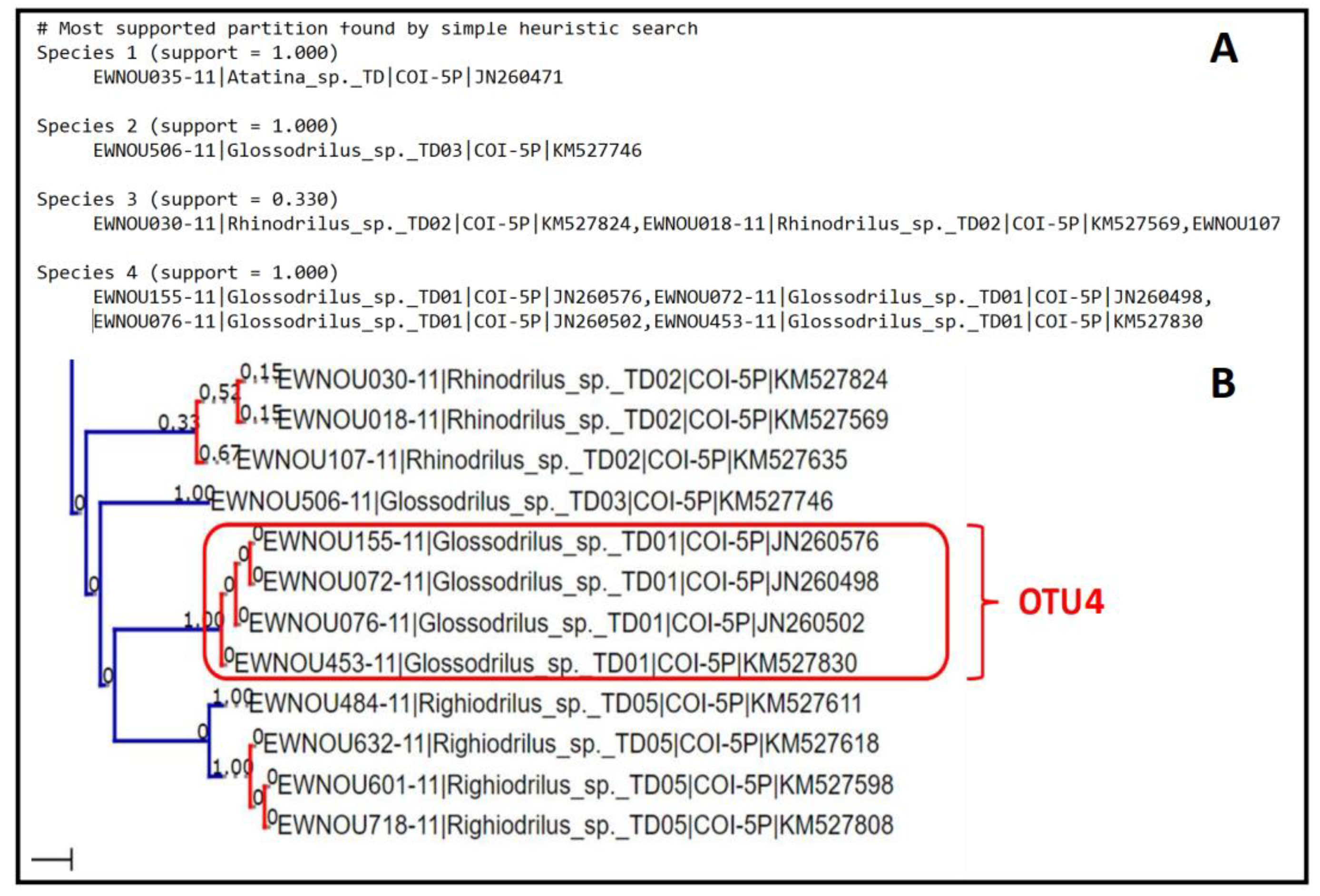
Each method provides some visualisation of the results usually in its own format, which constrains the possibilities of interpretation for the user. For the PTP method, the software returns a text file with the distribution of sequences in the different OTUs obtained (Figure 1A). It also provides a phylogenetic tree with a colour code on the branches to visualise the delimitations (blue and red). Indeed, all sequences after a red branch are gathered in the same OTU. The terminal branch remains blue in the case of singletons (i.e., OTU represented by a single sequence in the dataset) (Figure 1B).
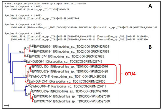
Figure 1.
Output results obtained with the PTP method: (A) extract from the text file showing the distribution of sequences from dataset 1 in the different OTUs; (B) extract from the output phylogenetic tree showing the distances between sequences and how they are distributed in the different OTUs.
GMYC only provides a phylogenetic tree with a color-coded system on the terminal branches to visualise OTUs; only singletons appear in black in this tree (Figure 2A). Note that the graphical quality is not optimized, and it is therefore necessary to return to the input tree, which has the same topology, in order to interpret the groupings of sequences into OTUs. As no text output is provided, it is necessary to manually transfer the OTU assignments into a spreadsheet so that they are available for further analysis.
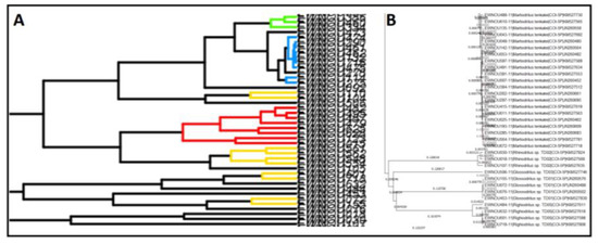
Figure 2.
Output results obtained with the GMYC method: (A) extract of the output tree of the GMYC method in which the color codes allow the visualisation of OTUs delimitations; (B) extract of the input tree of the dataset which allows a more efficient visualisation of the identity of the leaves on the GMYC output tree.
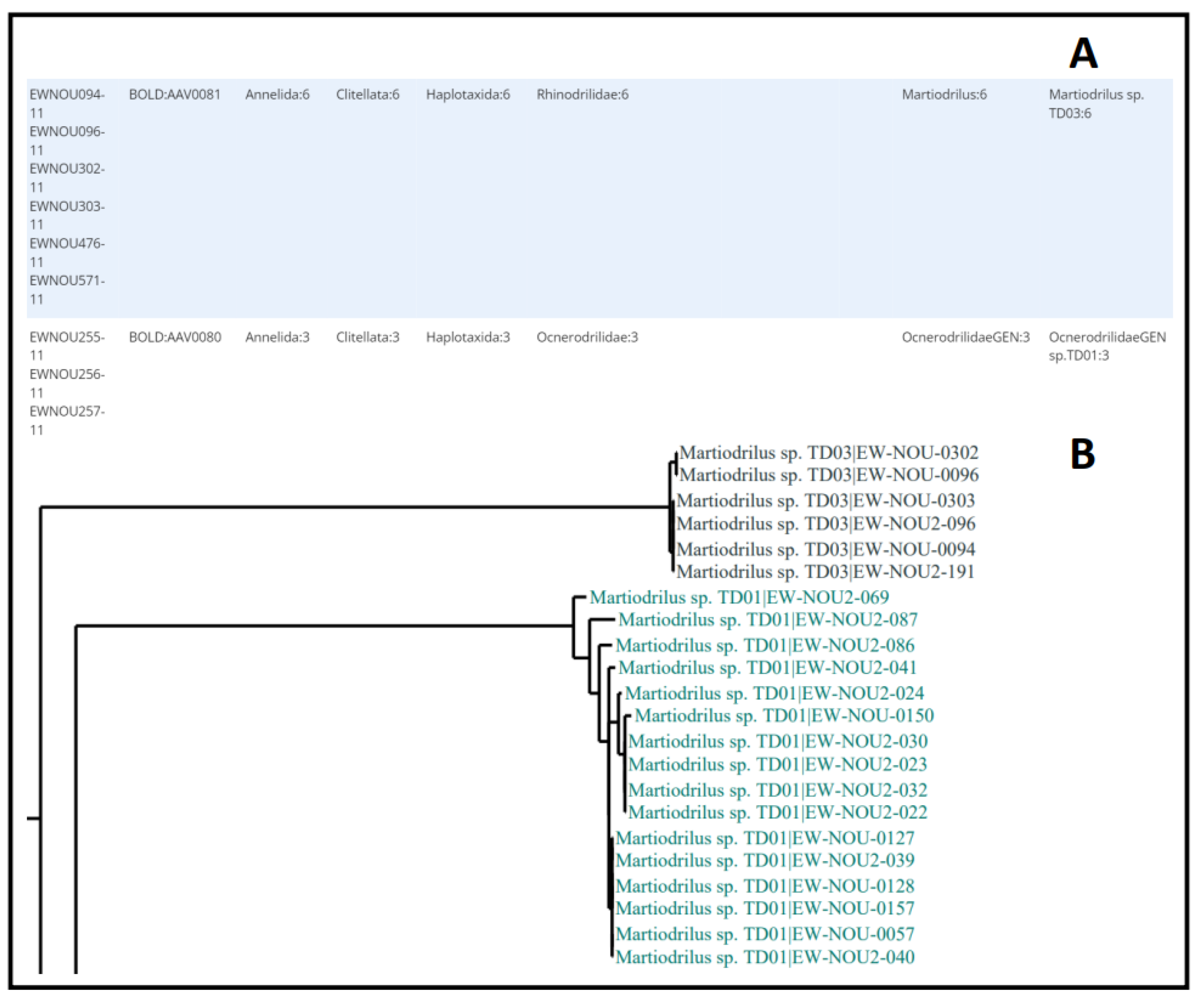
For the RESL method, the ‘clustering sequences’ tool implemented on BOLD allows the delimitation of OTUs from the sequences of a particular dataset. The software returns a table listing the sequences assigned to OTUs (Figure 3A). There is no graphical output, but the delimitation can then be completed by a neighbor joining tree that allows direct visualisation of the BINs (Figure 3B).
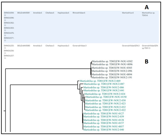
Figure 3.
Output results obtained with the RESL method: (A) extract from the file of sequences from dataset 1 distributed in the different OTUs; (B) extract from the neighbor joining tree obtained with the same sequences from the BOLD platform, showing the distances between sequences and the way they are organized in OTUs.
In the case of ABGD, the software gives a histogram showing the distribution of distance per pair of sequences (Figure 4A), which thus allows users to efficiently visualise the ‘barcode gap’. ABGD also provides an output showing the results of several delineations (Figure 4B). One of the input parameters (‘steps’) is the number of delineations that one wishes to obtain. For each delimitation, the software returns a text file that gives the distribution of sequences within the OTUs (Figure 4C).
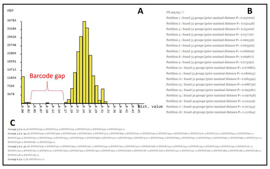
Figure 4.
Output results obtained with the ABGD method: (A) diagram showing the distribution of pairwise genetic distances (K2P) between the sequences of dataset 1; (B) list of the 10 delimitations according to the specific divergence value p; and (C) extract from the text file showing the distribution of the sequences of dataset 1 in the OTUs.
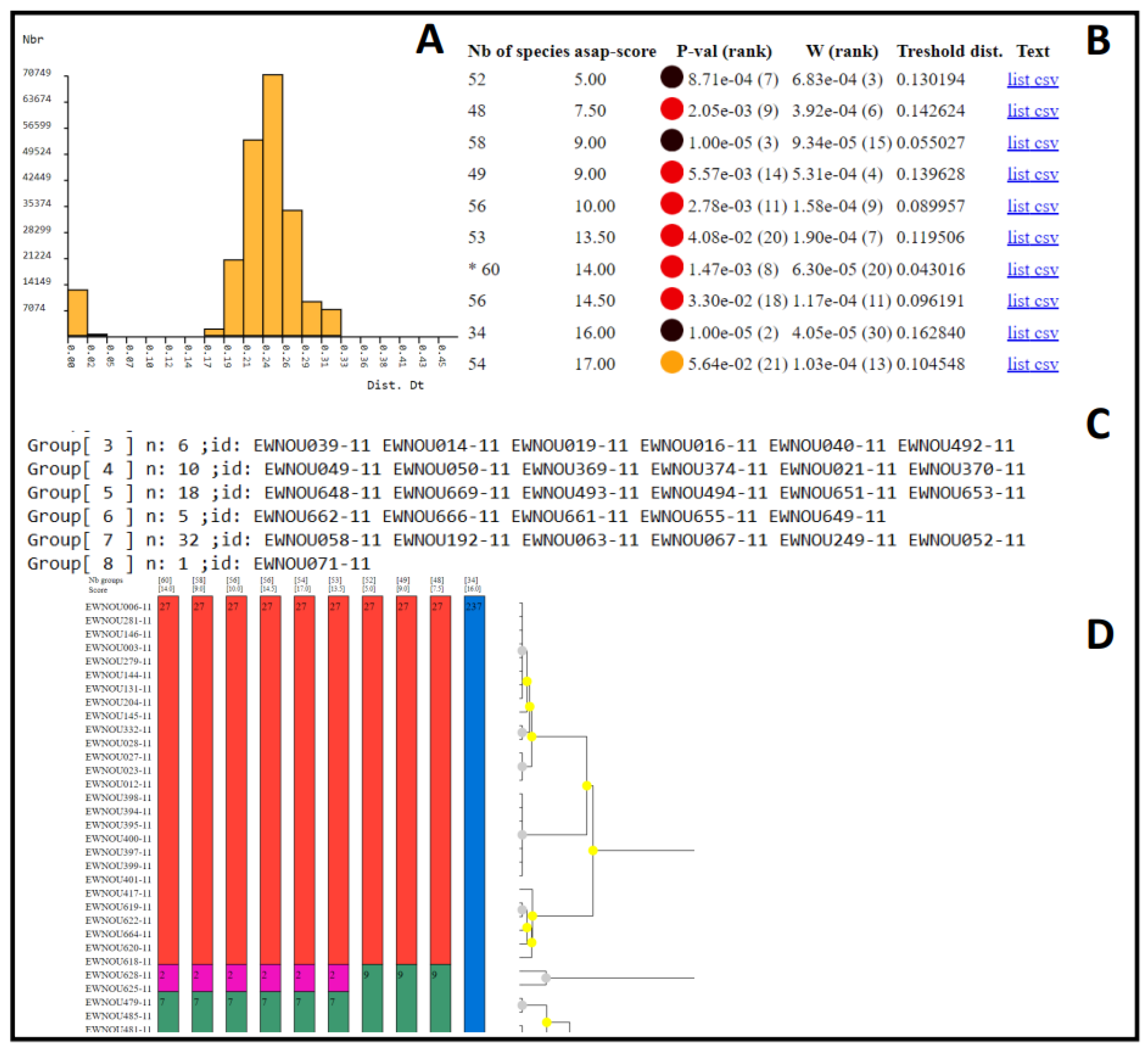
The ASAP software offers a similar but improved version of the ABGD output. It first produces a histogram showing the distribution of the intra- and inter-specific genetic distances and allowing the visualisation of the barcode-gap (Figure 5A). It also produces a summary table of the 10 best partitions with the highest ASAP scores (Figure 5B). For each of the partition, the number of OTUs is given, as well as the p-value and W-values that determine the ASAP score and the ‘threshold distance’, which is the limit value of genetic divergence for which two sequences are considered to belong to different OTUs. For each of the delimitations, a text file gives the distribution of sequences in the different OTUs (Figure 5C). Finally, the software provides a graphical output that allows the 10 proposed partitions to be visualised on an ultrametric clustering tree (Figure 5D).
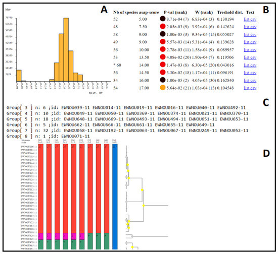
Figure 5.
Output results obtained with the ASAP method: (A) diagram showing the distribution of pairwise genetic distances (K2P) between the sequences of dataset 1; (B) list of the 10 delimitations with the best ASAP scores; (C) extract from the text file showing the distribution of sequences from dataset 1 in the OTUs; and (D) extract graphical output showing the different delimitations together with the ultrametric clustering tree; each column in D represents a partition, and the colors represent the OTUs.
3.4. Result Reliability
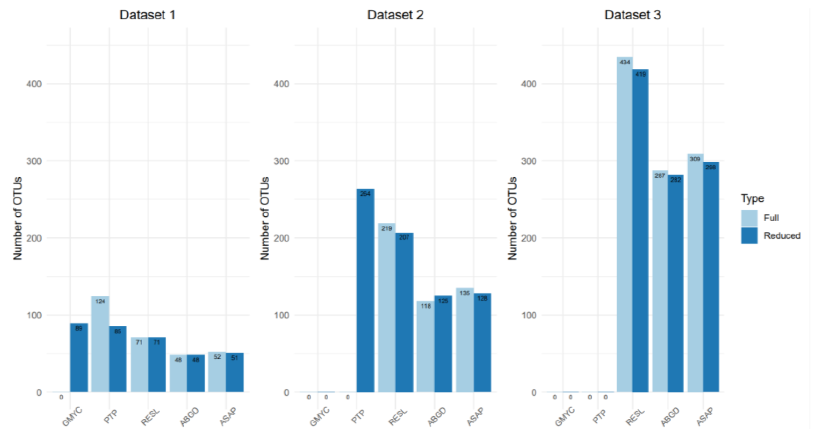
The number of OTUs obtained from the three datasets and with the different methods is shown in Figure 6. With the exception of the PTP method for the reduced dataset 2, the phylogenetic tree methods (GMYC and PTP) failed to successfully process datasets 2 and 3. The distance matrix methods (ABGD and ASAP) produced broadly similar results in terms of OTU number, and also produced a generally lower number of OTUs than the other methods.
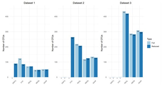
Figure 6.
Number of OTUs obtained from three datasets (both in their full version or after reduced to a single sequence per haplotype) with five different delineation methods.
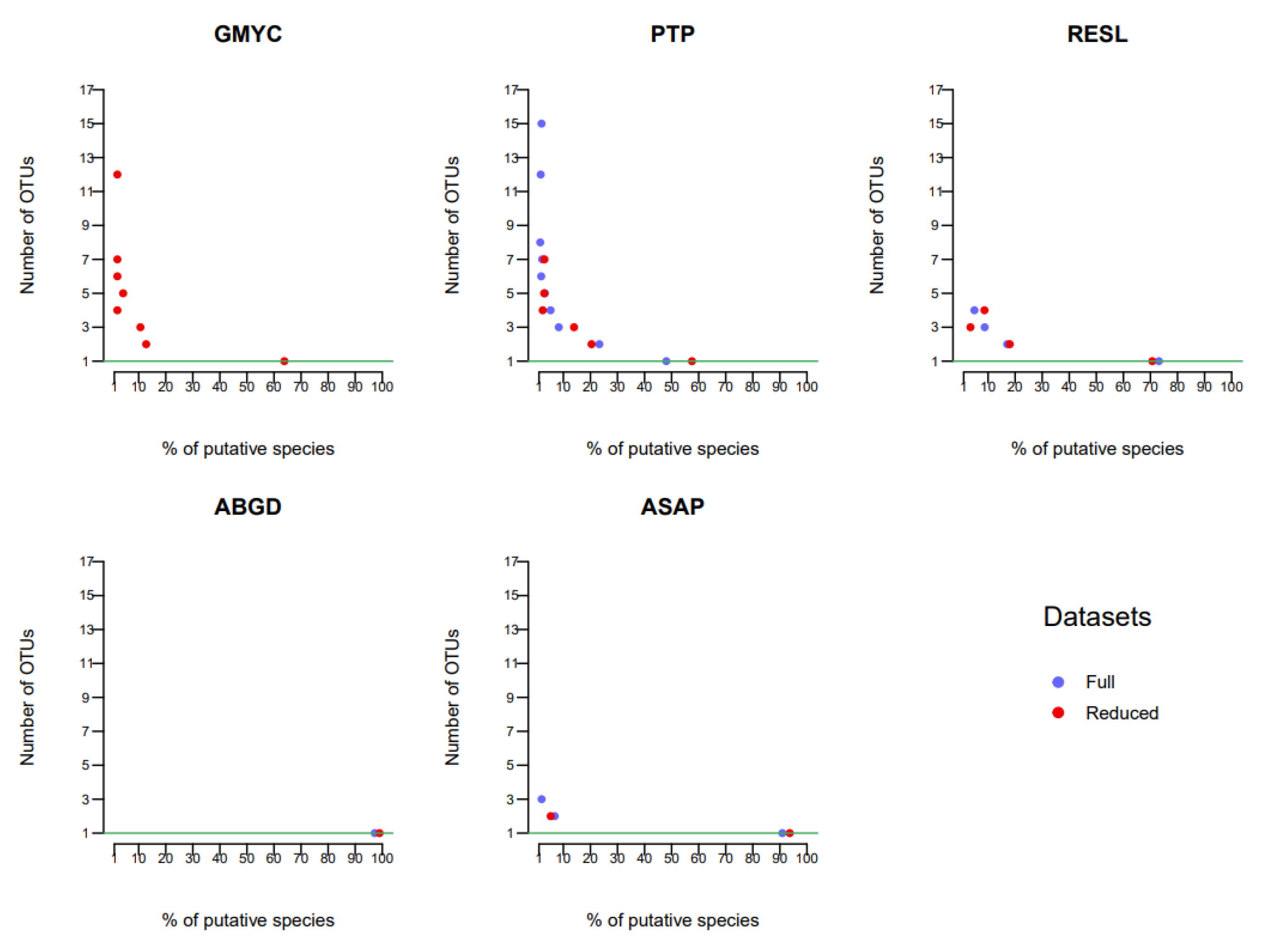
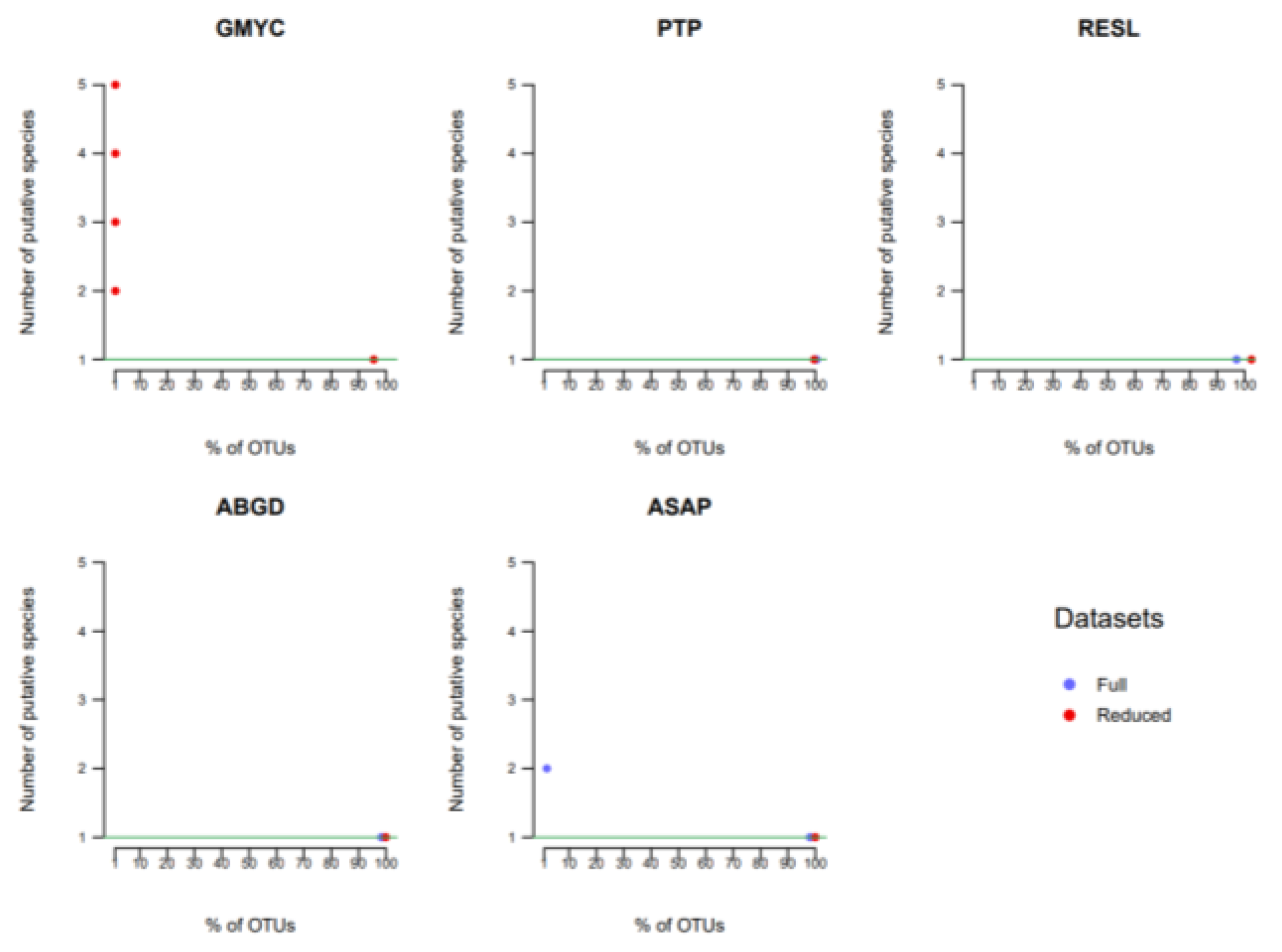
The mismatch rates obtained with the different methods for processing dataset 1 are shown in Figure 7 (for split mismatches) and Figure 8 (for merge mismatches). In general, the results obtained are quite similar whether the dataset is used in its full version or reduced to a single sequence per haplotype. We can also observe that merge mismatches are rather rare (only a few isolated cases with the ASAP and GMYC methods), and that the majority of mismatches correspond to splits. The tendency of the different methods to separate putative species into several OTUs is also extremely variable: it is null for ABGD, low for ASAP and RESL, but much higher for PTP and GMYC.
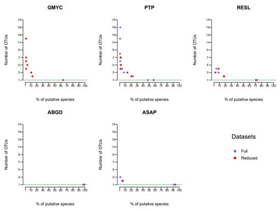
Figure 7.
Mismatch rates corresponding to splits (when a putative species is split into several OTUs) obtained while processing dataset 1 with the five delimitation methods. The graphs represent, for the dataset in its full version or after reduced to one sequence per haplotype, the proportion of putative species that are split by the different methods as a function of the magnitude of the mismatch (the number of OTUs resulting from the split). The dots on the horizontal green line indicate the proportion of putative species that are recovered in the OTU partitions (perfect match).
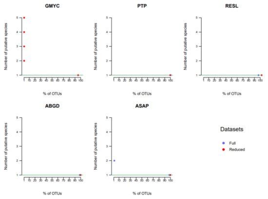
Figure 8.
Mismatch rates corresponding to merges (when several putative species are grouped into a single OTU) obtained while processing dataset 1 with the five delimitation methods. The graphs represent, for the dataset in its full version or after reduced to one sequence per haplotype, the proportion of OTUs obtained that correspond to a grouping of several putative species, as a function of the magnitude of the mismatch (the number of putative species that are grouped in a single OTU). The dots on the horizontal green line indicate the proportion of OTUs that correspond to a single putative species (perfect match).
Regardless of the delimitation method used, the majority of split mismatches correspond to cases where a putative species is split into two distinct OTUs. However, PTP and GMYC also generate over-split cases where a putative species can be split into more than three and up to 15 OTUs (in the case of an Ocnerodrilidae species with the PTP method). The PTP method generates the highest number of splits overall (Figure 7), with 52.1% mismatch for the full dataset and 43.8% mismatch for the reduced dataset. It is noteworthy that almost 50% of these mismatches correspond to splits in three or more OTUs. With the GMYC method, we also find this pattern with 37.5% of putative species split, 66.7% of which are in three or more OTUs. We also find one species split into 12 OTUs (Martiodrilus tenkatei) and four merges including 1 OTU grouping together five putative species that are taxonomically well separated from each other (Atatina sp. TD, Pontoscolex corethrurus, Pontoscolex sp. TD01, Pontoscolex sp. TD02, Wegeneriona sp. TD04).
For ASAP and RESL the number of mismatches generated by the processing of the reduced dataset is equal to or lower than that obtained with the full dataset. However, the identity of the putative species affected by these mismatches remains the same whichever dataset considered. On the other hand, a certain number of putative species are split after analysis of the complete dataset, whereas this is not the case with the reduced dataset. This is especially true for the RESL and ASAP models. With PTP, a higher proportion of mismatches is also observed when analysing the full dataset, but some putative species are also split after analysis of the reduced dataset whereas they are not with the full dataset (e.g., for Pontoscolex corethrurus and HaplotaxidaGEN sp. TD02). Finally, there are also differences in the magnitude of the mismatches, i.e., the number of OTUs resulting from the split of a given putative species. For example, the putative species OcnerodrilidaeGEN_sp.TD01 is split into 4 OTUs by the PTP method applied to the reduced dataset, whereas it is split into 15 OTUs with the full dataset.
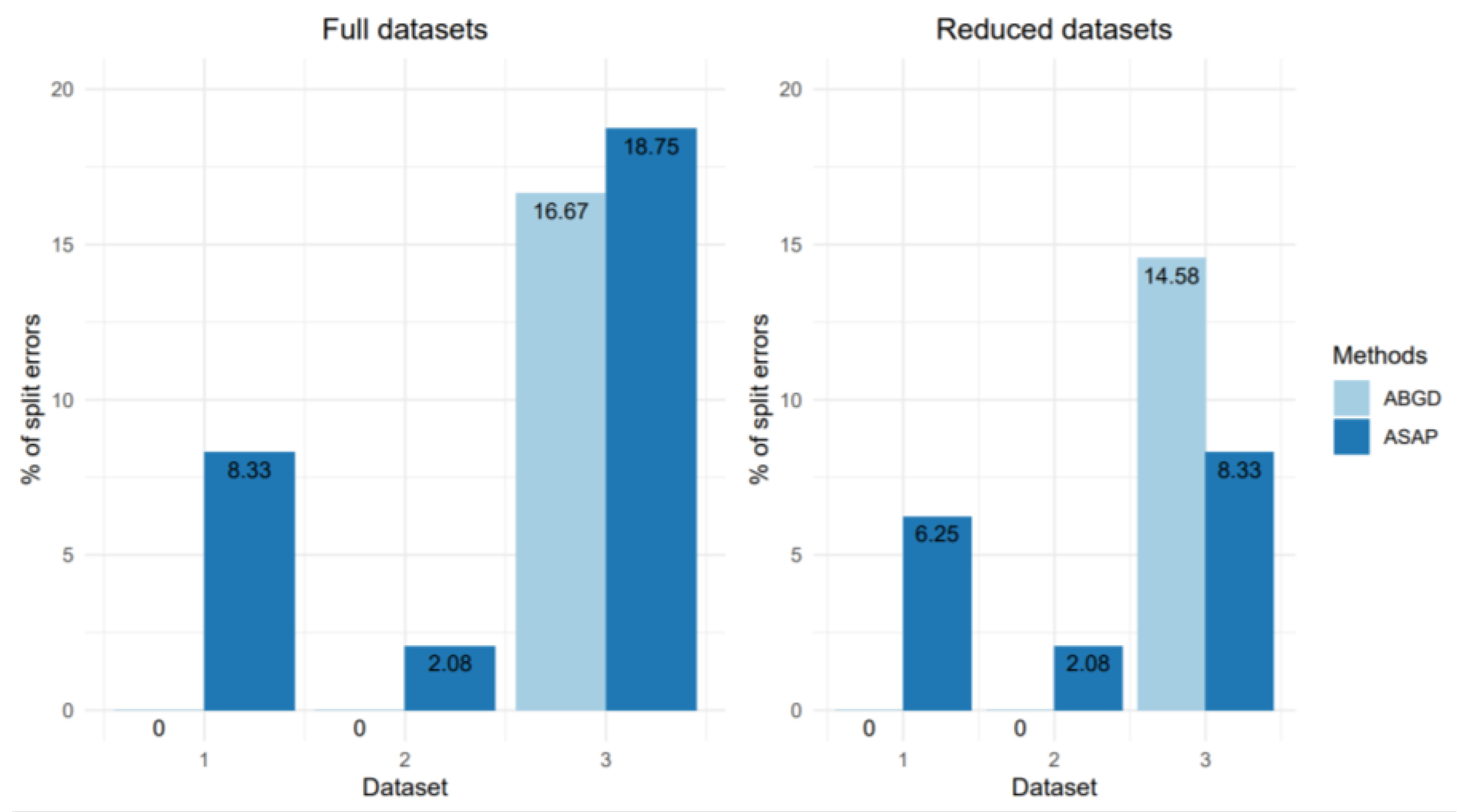
In general, the analysis of dataset 1 shows ABGD and ASAP to be the two most reliable methods when it comes to analyzing less than one thousand sequences. In a second step, we compared the reliability of the results obtained by these two methods with datasets 2 and 3 which contain a larger number of sequences (Figure 9 and Figure 10). With dataset 2, no split is observed using the ABGD method, and a few merge mismatches appear with the full dataset, whereas with ASAP a single split is observed for the putative species Neogaster sp.TD03 independent of the dataset version. For dataset 3, the number of mismatches is equivalent between the two methods when the full dataset is used. However, the AGBD method produces more split and merge mismatches when applied to the dataset reduced to one sequence per haplotype.

Figure 9.
Mismatch rates corresponding to splits (when a putative species is split into several OTUs) observed with the three datasets processed with the ABGD and ASAP methods. The graphs represent, for the dataset in its full version or after reduced to one sequence per haplotype, the proportion of putative species that are split by the different methods.
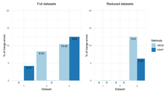
Figure 10.
Mismatch rates corresponding to merges (when several putative species are grouped into a single OTU) obtained by processing dataset 1 with the ABGD and ASAP methods. The graphs represent, for the dataset in its full version or after reduced to one sequence per haplotype, the proportion of OTUs obtained that correspond to a grouping of several putative species.
4. Discussion
The study of earthworm diversity faces the limits of traditional morphology-based taxonomy: the lack of stable and easily observable morphological characters, cases of cryptic diversity or, on the contrary, of the high level of phenotypic variability in certain species and the absence of diagnostic characters at juvenile stages [3]. In order to overcome this taxonomic barrier, DNA barcoding has emerged as a useful tool for research of earthworm taxonomy, systematics, evolution and ecology [1,3]. However, its usefulness relies largely on the reliability of the OTU delineations that can be obtained from DNA barcodes, in other words the ability to obtain OTUs that best represent the biological species sampled. The choice of the OTU delineation method is therefore crucial and needs to be made with knowledge of the specificities of earthworm COI DNA barcode variability. Actually, the best approach would be to systematically and comparatively use several methods [30], if possible on multi-locus data sets. However, with the widespread use of DNA barcoding and NGS approaches, more and more large monolocus datasets are being produced, making an objective comparison of OTU delineation methods necessary. We tested five of the most commonly used delineation methods. While most studies that have performed this type of comparison have focused on the relevance of the delineations [13,31], we went further by also considering the efficiency of the software in terms of computation time, the nature and usability of the output, as well as the nature of the prior knowledge required (Paz and Crawford 2012) [32].
The upstream preparation of phylogenetic trees is a major constraint of both the GMYC and PTP methods, especially in the case of GMYC, for which a molecular clock has to be selected to obtain dated trees. In addition to the time required and the complexity of this step for neophytes, it requires additional a priori hypotheses, which can represent a source of potential errors. Distance matrix methods avoid this difficulty as they use relatively untransformed data. This is important because many users of DNA barcodes come from the world of ecology or taxonomy, and do not necessarily have the experience and technical skills to manipulate phylogenetic trees.
Some applications seem more complex when it comes to setting input parameters. In particular, PTP and ABGD require the input of five and six different parameters, respectively, some of which may be difficult to enter. The usually high values of the barcode gap in earthworms [33,34] mean that the levels of Pmin and Pmax must be set far apart, thus increasing the number of possible delimitations for a fixed ‘step’, and increasing the time required for analysis. For GMYC and ASAP, only one parameter needs to be entered before the analysis, and none is required for the RESL method. Thus, we clearly distinguish the approaches based on phylogenetic trees built upstream (PTP and GMYC) from three others (RESL, ABGD and ASAP) for which this prerequisite is not necessary. Of these, RESL and ASAP are the methods that require the least prior knowledge and do not require any a priori assumptions.
Regarding computational time, RESL, ABGD and ASAP methods are clearly more efficient than methods using phylogenetic trees. This is particularly evident when the dataset to be processed is large. In our comparison, the computation time of the latter methods is consistently longer than that of the distance matrix methods, and they fail to converge and delimit OTUs when the number of sequences to be processed was large. The computational time required with the distance matrix methods, which is already comparatively much shorter, can be further reduced by downloading ABGD or ASAP and performing the analyses locally. For our study, we decided to work with the web interface to allow objective comparisons with GMYC and PTP.
The five methods tested in our study differ from each other in terms of the outputs they produce. PTP, RESL, ABGD and ASAP provide a table with the distribution of sequences within OTUs. This output is lacking for GMYC, which is a limitation for the use of the method. In fact, obtaining this table is necessary to allow for an efficient use of OTUs in ecological studies [15,16] or as support for phylogenetic reconstruction [35]. ASAP, PTP, GMYC and RESL (via the options offered by the BOLD platform) also produce a clustering tree associated with a colour system allowing the graphical visualisation of OTUs. With GMYC, however, this tree is insufficient as labels on the terminal branches are impossible to read. An important advantage of ASAP over other the other methods is that it offers a single clustering tree on which the 10 best delimitations are mapped. This option, as well as the ASAP score that accompanies each delimitation, allows the user to efficiently compare the different proposals with other sources of information (e.g., morphology, ecology, distribution) in order to select the most relevant through an integrative taxonomy approach (as for example in Decaëns et al., 2016 [15]).
Our results suggest that at least in the case of large earthworm barcode dataset, distance matrix approaches are more reliable than those based on a phylogenetic approach. In our study, the PTP and GMYC methods produce numerous splits, probably due to bias in the reconstruction of ultrametric trees. Indeed, it is acknowledged that GMYC tends to separate biological species into several OTUs due to excessive lineage splitting [13,32]. The RESL method is a good example of a method that is effective for certain taxa such as insects [8], but weakly adapted to the specificities of our dataset. Indeed, the graph approach seems unable to correctly identify the barcode gap in the case of earthworms in which COI is deeply divergent (i.e., barcode gap generally around 14% [3,33,34]). Therefore, our results suggest that the BINs as proposed automatically in the BOLD platform should be considered with caution for taxa with deep COI intraspecific variability. Compared to the other methods, ABGD and ASAP emerge as the two most reliable methods. ABGD gives somewhat better results for small datasets, but this difference fades for larger datasets. Furthermore, ABGD tends to artificially group some phylogenetically distant species in certain OTUs, a bias that has already been noticed in previous studies such as Pentinsaari et al. on beetle groups [36]. In comparison, ASAP produces a much lower number of merge mismatches, especially when the dataset is reduced to a single sequence per haplotype.
5. Conclusions
Phylogenetic approaches are less suitable for delineating OTUs from DNA barcodes in earthworms, especially for datasets with a large number of sequences. The computation times are unreasonable, they often fail to converge, and they also show a strong tendency to oversplit species, making OTU delineation difficult to use in any type of study. Therefore, distance matrix methods seem preferable. RESL is easy to use as it is implemented directly on the BOLD platform, but this method also has a clear tendency to oversplit earthworm species. ABGD and ASAP are less prone to split and merge mismatches, and both have short completion times. ASAP requires less prior knowledge for model parameterisation. In addition, it provides a graphical output with the different OTUs delimitations visualised directly on a clustering tree, which is easy to understand and represents an effective aid to the interpretation of the results. In contrast, ABGD only provides a simple text file with the distribution of sequences within the OTUs. Finally, ASAP also differs from ABGD in that it has a much lower tendency to generate mismatches, particularly merge mismatches when analysing large datasets.
Author Contributions
Conceptualization, T.D., M.H. and A.G.; methodology, A.G., B.P. and T.D.; formal analysis, A.G., B.P. and M.-E.M.; writing—original draft preparation, A.G.; writing—review and editing, T.D., M.H., D.F.M., D.S., B.P. and M.-E.M.; supervision, T.D. and M.H.; funding acquisition, T.D. and D.S. All authors have read and agreed to the published version of the manuscript.
Funding
This research was funded the Agence Nationale de la Recherche (CEBA: ANR-10-LABX-25-01; TULIP: ANR-10-LABX-41) and Centre National de la Recherche Scientifique (INEE-APEGE-2013: DJ/ST/IP/2013/D-112).
Institutional Review Board Statement
Not applicable.
Informed Consent Statement
Not applicable.
Data Availability Statement
DS-EWFG2022 dx.doi.org/10.5883/DS-EWFG2022.
Acknowledgments
We are grateful to the Parc Amazonien de Guyane (http://www.parcamazonien-guyane.fr), the Réserve Naturelle des Nouragues (https://www.nouragues.fr/), and the Réserve Naturelle de la Trinité (http://www.reserve-trinite.fr/) for collecting authorizations and for financial and logistical support. This work was supported by ‘Investissement d’Avenir’ grants managed by the Agence Nationale de la Recherche (CEBA: ANR-10-LABX-25-01; TULIP: ANR-10-LABX-41). In the Mitaraka region, material was collected as part of ‘Our Planet Reviewed’ Guyane-2015 expedition, which was organized by the Muséum national d’Histoire naturelle (MNHN, Paris) and Pro-Natura international in collaboration with the Parc Amazonien de Guyane, with financial support of the European Regional Development Fund (ERDF), the Conseil régional de Guyane, the Conseil général de Guyane, the Direction de l’Environnement, de l’Aménagement et du Logement and the Ministère de l’Education Nationale, de l’Enseignement Supérieur et de la Recherche. Additional funding was provided by the Trinité Natural Reserve. At the Nouragues, the project was supported by two grants CNRS Nouragues’ 2010 and 2011. DNA barcoding was supported as part of the International Barcode of Life program, the Centre National de la Recherche Scientifique (INEE-APEGE-2013: DJ/ST/IP/2013/D-112) and the Canada First Research Excellence Fund.
Conflicts of Interest
The authors declare no conflict of interest.
References
- Marchán, D.F.; Decaëns, T.; Domínguez, J.; Novo, M. Perspectives in earthworm molecular phylogeny: Recent advances in Lumbricoidea and standing questions. Diversity 2022, 14, 30. [Google Scholar] [CrossRef]
- Hebert, P.D.N.; Ratnasingham, S.; de Waard, J.R. Barcoding animal life: Cytochrome c oxidase subunit 1 divergences among closely related species. Proc. R. Soc. B Biol. Sci. 2003, 270 (Suppl. 1), S96–S99. [Google Scholar] [CrossRef]
- Decaëns, T.; Porco, D.; Rougerie, R.; Brown, G.G.; James, S.W. Potential of DNA barcoding for earthworm research in taxonomy and ecology. Appl. Soil Ecol. 2013, 65, 35–42. [Google Scholar] [CrossRef]
- Zhou, X.; Frandsen, P.B.; Holzenthal, R.W.; Beet, C.R.; Bennett, K.R.; Blahnik, R.J.; Bonada, N.; Cartwright, D.; Chuluunbat, S.; Cocks, G.V.; et al. The Trichoptera barcode initiative: A strategy for generating a species-level Tree of Life. Philos. Trans. R. Soc. B 2016, 371, 20160025. [Google Scholar] [CrossRef]
- Bass, D.; Czech, L.; Williams, B.A.P.; Berney, C.; Dunthorn, M.; Mahé, F.; Torruella, G.; Stentiford, G.D.; Williams, T.A. Clarifying the relationships between Microsporidia and Cryptomycota. J. Eukaryot. Microbiol. 2018, 65, 773–782. [Google Scholar] [CrossRef]
- Pons, J.; Barraclough, T.G.; Gomez-Zurita, J.; Cardoso, A.; Duran, D.P.; Hazell, S.; Kamoun, S.; Sumlin, W.D.; Vogler, A.P. Sequence-based species delimitation for the DNA taxonomy of undescribed insects. Syst. Biol. 2006, 55, 595–609. [Google Scholar] [CrossRef] [PubMed]
- Zhang, J.; Kapli, P.; Pavlidis, P.; Stamatakis, A. A general species delimitation method with applications to phylogenetic placements. Bioinformatics 2013, 29, 2869–2876. [Google Scholar] [CrossRef] [PubMed]
- Ratnasingham, S.; Hebert, P.D.N. A DNA-based registry for all animal species: The Barcode Index Number (BIN) system. PLoS ONE 2013, 8, e66213. [Google Scholar] [CrossRef] [PubMed]
- Puillandre, N.; Lambert, A.; Brouillet, S.; Achaz, G. ABGD, ABGD, Automatic Barcode Gap Discovery for primary species delimitation. Mol. Ecol. 2012, 21, 1864–1877. [Google Scholar] [CrossRef]
- Puillandre, N.; Brouillet, S.; Achaz, G. ASAP: Assemble species by automatic partitioning. Mol. Ecol. Resour. 2021, 21, 609–620. [Google Scholar] [CrossRef]
- Nei, M.; Maruyama, T.; Chakraborty, R. The bottleneck effect and genetic variability in populations. Evolution 1975, 29, 1–10. [Google Scholar] [CrossRef] [PubMed]
- Bazin, E.; Glémin, S.; Galtier, N. Population size does not influence mitochondrial genetic diversity in animals. Science 2006, 312, 570–572. [Google Scholar] [CrossRef] [PubMed]
- Kekkonen, M.; Hebert, P.D.N. DNA barcode-based delineation of putative species: Efficient start for taxonomic workflows. Mol. Ecol. Resour. 2014, 14, 706–715. [Google Scholar] [CrossRef]
- Lees, D.C.; Kawahara, A.Y.; Rougerie, R.; Ohshima, I.; Kawakita, A.; Bouteleux, O.; De Prins, J.; Lopez-Vaamonde, C. DNA barcoding reveals a largely unknown fauna of Gracillariidae leaf-mining moths in the Neotropics. Mol. Ecol. Resour. 2014, 14, 286–296. [Google Scholar] [CrossRef]
- Decaëns, T.; Porco, D.; James, S.W.; Brown, G.G.; Chassany, V.; Dubs, F.; Dupont, L.; Lapied, E.; Rougerie, R.; Rossi, J.-P.; et al. DNA barcoding reveals diversity patterns of earthworm communities in remote tropical forests of French Guiana. Soil Biol. Biochem. 2016, 92, 171–183. [Google Scholar] [CrossRef]
- Maggia, M.-E.; Decaëns, T.; Lapied, E.; Dupont, L.; Roy, V.; Schimann, H.; Orivel, J.; Murienne, J.; Baraloto, C.; Cottenie, K.; et al. At each site its diversity: DNA barcoding reveals remarkable earthworm diversity in neotropical rainforests of French Guiana. Appl. Soil Ecol. 2021, 164, 103932. [Google Scholar] [CrossRef]
- Folmer, O.; Black, M.; Hoeh, W.; Lutz, R.; Vrijenhoek, R. DNA primers for amplification of mitochondrial cytochrome c oxidase subunit I from diverse metazoan invertebrates. Mol. Mar. Biol. Biotechnol. 1994, 3, 294–299. [Google Scholar]
- Hebert, P.D.N.; Penton, E.H.; Burns, J.M.; Janzen, D.H.; Hallwachs, W. Ten species in one: DNA barcoding reveals cryptic species in the neotropical skipper butterfly Astraptes fulgerator. Proc. Natl. Acad. Sci. USA 2004, 101, 14812–14817. [Google Scholar] [CrossRef]
- Hajibabaei, M.; Janzen, D.H.; Burns, J.M.; Hallwachs, W.; Hebert, P.D.N. DNA barcodes distinguish species of tropical Lepidoptera. Proc. Natl. Acad. Sci. USA 2006, 103, 968–971. [Google Scholar] [CrossRef]
- Villesen, P. FaBox: An online toolbox for fasta sequences. Mol. Ecology Notes 2007, 7, 965–968. [Google Scholar] [CrossRef]
- Tamura, K.; Stecher, G.; Kumar, S. MEGA11: Molecular Evolutionary Genetics Analysis version 11. Mol. Biol. Evol. 2021, 38, 3022–3027. [Google Scholar] [CrossRef] [PubMed]
- Paradis, E.; Schliep, K. ape 5.0: An environment for modern phylogenetics and evolutionary analyses in R. Bioinformatics 2019, 35, 526–528. [Google Scholar] [CrossRef]
- Yule, G.U. A mathematical theory of evolution, based on the conclusions of Dr. J. C. Willis, F.R.S. Philos. Trans. R. Soc. B 1925, 213, 21–87. [Google Scholar]
- Nee, S.; Holmes, E.C.; May, R.M.; Harvey, P.H. Extinction rates can be estimated from molecular phylogenies. Philos. Trans. R. Soc. B 1994, 344, 77–82. [Google Scholar] [CrossRef]
- Kingman, J.F.C. The coalescent. Stoch. Process. Their Appl. 1982, 13, 235–248. [Google Scholar] [CrossRef]
- Hudson, R.R. Gene genealogies and the coalescent process. Oxf. Surv. Evol. Biol. 1990, 7, 1–44. [Google Scholar]
- Monaghan, M.T.; Wild, R.; Elliot, M.; Fujisawa, T.; Balke, M.; Inward, D.J.G.; Lees, D.C.; Ranaivosolo, R.; Eggleton, P.; Barraclough, T.G.; et al. Accelerated species inventory on Madagascar using Coalescent-Based Models of species delineation. Syst. Biol. 2009, 58, 298–311. [Google Scholar] [CrossRef]
- Kapli, P.; Lutteropp, S.; Zhang, J.; Kobert, K.; Pavlidis, P.; Stamatakis, A.; Flouri, T. Multi-rate Poisson Tree Processes for single-locus species delimitation under Maximum Likelihood and Markov Chain Monte Carlo. Bioinformatics 2017, 33, 1630–1638. [Google Scholar] [CrossRef]
- Ratnasingham, S.; Hebert, P.D.N. BARCODING: Bold: The Barcode of Life Data System. Mol. Ecol. Notes 2007, 7, 355–364. [Google Scholar] [CrossRef]
- Carstens, B.C.; Pelletier, T.A.; Reid, N.M.; Satler, J.D. How to fail at species delimitation. Mol. Ecol. 2013, 22, 4369–4383. [Google Scholar] [CrossRef] [PubMed]
- Luo, A.; Ling, C.; Ho, S.Y.W.; Zhu, C.-D. Comparison of methods for molecular species delimitation across a range of speciation scenarios. Syst. Biol. 2018, 67, 830–846. [Google Scholar] [CrossRef]
- Paz, A.; Crawford, A.J. Molecular-based rapid inventories of sympatric diversity: A comparison of DNA barcode clustering methods applied to geography-based vs clade-based sampling of amphibians. J. Biosci. 2012, 37, 887–896. [Google Scholar] [CrossRef] [PubMed]
- Chang, C.-H.; James, S. A critique of earthworm molecular phylogenetics. Pedobiologia 2011, 54, S3–S9. [Google Scholar] [CrossRef]
- Rougerie, R.; Decaëns, T.; Deharveng, L.; Porco, D.; James, S.W.; Chang, C.-H.; Richard, B.; Potapov, M.; Suhardjono, Y.; Hebert, P.D.N. DNA barcodes for soil animal taxonomy. Pesqui. Agropecu. Bras. 2009, 44, 789–802. [Google Scholar] [CrossRef]
- Song, C.; Wang, Q.; Zhang, R.; Sun, B.; Wang, X. Exploring the utility of DNA barcoding in species delimitation of Polypedilum (Tripodura) non-biting midges (Diptera: Chironomidae). Zootaxa 2016, 4079, 534. [Google Scholar] [CrossRef] [PubMed]
- Pentinsaari, M.; Vos, R.; Mutanen, M. Algorithmic single-locus species delimitation: Effects of sampling effort, variation and nonmonophyly in four methods and 1870 species of beetles. Mol. Ecol. Resour. 2017, 17, 393–404. [Google Scholar] [CrossRef] [PubMed]
Publisher’s Note: MDPI stays neutral with regard to jurisdictional claims in published maps and institutional affiliations. |
© 2022 by the authors. Licensee MDPI, Basel, Switzerland. This article is an open access article distributed under the terms and conditions of the Creative Commons Attribution (CC BY) license (https://creativecommons.org/licenses/by/4.0/).

