Abstract
Fisheries management has historically focused on the population elasticity of target fish based primarily on demographic modeling, with the key assumptions of stability in environmental conditions and static trophic relationships. The predictive capacity of this fisheries framework is poor, especially in closed systems where the benthic diversity and boundary effects are important and the stock levels are low. Here, we present a probabilistic model that couples key fish populations with a complex suite of trophic, environmental, and geomorphological factors. Using 41 years of observations we model the changes in eastern Baltic cod (Gadus morhua), herring (Clupea harengus), and Baltic sprat (Sprattus sprattus balticus) for the Baltic Sea within a Bayesian network. The model predictions are spatially explicit and show the changes of the central Baltic Sea from cod- to sprat-dominated ecology over the 41 years. This also highlights how the years 2004 to 2014 deviate in terms of the typical cod–environment relationship, with environmental factors such as salinity being less influential on cod population abundance than in previous periods. The role of macrozoobenthos abundance, biotopic rugosity, and flatfish biomass showed an increased influence in predicting cod biomass in the last decade of the study. Fisheries management that is able to accommodate shifting ecological and environmental conditions relevant to biotopic information will be more effective and realistic. Non-stationary modelling for all of the homogeneous biotope regions, while acknowledging that each has a specific ecology relevant to understanding the fish population dynamics, is essential for fisheries science and sustainable management of fish stocks.
1. Introduction
Ecosystem-based modeling approaches to fisheries management require models that can include the fundamental interaction present in the fisheries systems [1]. Even for relatively simple fisheries regions, such as the Baltic Sea, models can be improved if they account for localized diversity, species interactions at chosen trophic levels, environmental drivers, and human pressures [2]. Indeed, many models have extended their complexity to achieve this level of comprehension [3,4]. Despite these advances, there still exists a mismatch between modeling output and fisheries management—particularly in the spatial realm of marine reserve design, local seasonal closures, and real-time probabilistic assessment of fish biomass given field observations. Many fisheries models, despite containing many complex interaction components, still consider the fisheries ecosystem as a single homogeneous resource pool [5,6]. Spatial interactions of biota with the habitat and benthic structure are simplified or ignored in order to maintain traction with complicated mechanistic models [7].
Evidence of critical transitions occurring in marine ecosystems is dominated by coastal and inland sea systems [8]. The role of benthic dynamics in determining the character of the ecosystem dynamics, due to environmental fluctuations and the interaction with biotic elements, is well known [9,10], but remains challenging from a modelling perspective [7,11]. At one level, the mechanistic models lack the suitable experimental and observational data to determine the parameters for such a responsive system. On another level, the modeling frameworks that are often used struggle to include spatial processes—especially in continuous-time logistic models [12]. This is primarily due to the difficulty in defining the interaction suite for each habitat type and the mechanics of interaction processes between habitat zones.
In general, the term habitat has been widely used in relation to areas that are homogeneous in terms of their geophysical environment [13]. Therefore, in these cases, no information on the biota in that area is required. However, in this paper, we refer to the concept of biotopes, which are homogeneous units that are characterized by a typical species assemblage that exists in the geophysical environment [13]. For spatial mapping and conservation purposes, it is of fundamental importance to include biotope classes (distinct units with a homogeneous species composition) that are representative of their distributions, and to adapt the scale of observation and modelling to the scale of the patches that they form.
New modelling approaches are being explored that limit model complexity while maintaining predictive skill, negotiating uncertainty limits, and offering spatially valid explicit estimates of fisheries dynamics [7]. One such approach is to base the predictions on correlations between observations over space and time, rather than formulate a set of precise interaction equations. Correlations in a trophodynamic systems do not necessarily directly equate to metabolic, behavioral, or ecological processes, but the trade-off is the ability to predict with increased precision in a diverse and uncertain environment [10]. The trade-off between limiting models to well-defined causation links versus expanded models based on including correlations can be critical to management imperatives.
Bayesian Networks
Bayesian networks (BNs) offer the capacity to encompass complex interactions of disparate data types within a probabilistic framework with only a few limitations [14,15,16,17,18]. Bayes’ rule combined with the chain rule enables the propagation of conditional probability throughout a network structure. The network design is typically the result of expert opinion, although algorithms exist to formulate a possible structure through analysis of correlations. The parameterization of a model is achieved through the inclusion of observational cases that fully or partially describe a system’s state. The more cases used to inform the model’s conditional probabilities, the more accurate the predictions, but algorithms such as expectation maximization can assist in adjusting for missing data. Expert opinion, equations, and numerical (i.e., continuous, discrete, and censored) and categorical data can be included in the model, which is particularly useful for models of socioecological systems such as fisheries [19,20].
The development of a BN for a system that has been comprehensively observed for many decades while undergoing rapid change was an outstanding opportunity not only to increase knowledge of ecosystem dynamics, but also to advance fisheries ecosystem modeling. The Baltic Sea was such a system, with records of fishing catches combined with changing environmental conditions and fluctuating biota [19,20,21]. Such changes induced a fishery- and climate-induced regime shift that changed the food web from being dominated by the predator eastern Baltic cod (Gadus morhua, hereafter referred to as cod) to an alternative configuration dominated by planktivorous fish, e.g., Baltic sprat (Sprattus sprattus balticus) [22,23]. Even after the reduction in the cod catch, several biological changes occurred to the cod stock [24], which did not recover. Critically, the benthic pelagic coupling was particularly important in the Baltic Sea (largely due to the shallow nature of the sea), and also the young cod were dependent on benthic prey (the availability of which was closely linked to hypoxia) [21,25]. In order to better understand the dynamics of the cod that could help foresee their evolution and, therefore, aid in their management, thus-far overlooked pieces of information are needed. One of these could be represented by spatially explicit habitat information in relation to the cod stock dynamics [26]. Spatial dynamics across habitats or better biotopes are very important [27], and can have major effects on marine food webs [28].
Here, we present a spatially explicit trophodynamic model for the Baltic Sea based on 41 years of observations, including structural, environmental, and trophic data. With this model we answer two questions: (1) Are changes in diversity through alteration of biotopic conditions the key to shaping cod dynamics? (2) Are trophic, environmental, and biotopic feedbacks—and, consequently, cod biomasses—non-stationary?
2. Materials and Methods
2.1. Baltic Sea Study Area
The Baltic Sea (Figure 1) is an inland sea measuring 393,000 km2 and with a mean depth of only 54 m. The most significant environmental gradient is the surface salinity, which declines to almost fresh water in the innermost and northernmost areas. A highly saline region in the deeper locations causes stagnation of the bottom waters; the 85 million residents living in the adjacent catchments exacerbate this stagnation [29]. The latitudinal span from 53 N to 66 N creates a temperature gradient resulting in large variations from summer to winter. In general, the depth, substrate, wave exposure, and salinity gradient determine the benthic composition [30]. Habitat zones based on these factors with six levels of resolution were modeled by Wikstrom et al. [30]. Associated fisheries have concentrated on a diverse range of species, but primarily dominated by cod, herring, and sprat [31]. The collapse of the Baltic cod fisheries in the 1980s highlighted the transition of the Baltic Sea to an alternative state dominated by the commercially less valuable herring and sprat [21,32].
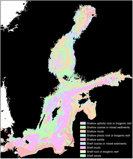
Figure 1.
Biotopes of the Baltic Sea, showing the polygons grouped into 9 categories [30].
2.2. Modeling Framework
To address the question regarding the factors influencing cod biomass, we needed a model framework that integrates environmental and structural components into a trophic network with the inclusion of fisheries’ catch influences. Motivating this model design were two practical limitations: Firstly, the variables included in the model needed to be based on raw observational data rather than model outputs, in order to minimize bias towards contemporary modeling approaches. Secondly, the spatial scale of the model needed to reflect the Baltic Sea management requirements yet concede to the spatial and temporal resolution of the observational data. The BN model is scale-invariant, but the prediction outputs are required to fit a spatial scale that can be mapped. The units of analysis selected were the EUSeaMap biotope polygons that vary in size and shape throughout the Baltic Sea [30]. This has the advantage that adjacent homogeneous areas (based on the classification level) could be merged into a larger area with a higher likelihood of being coincident with observational data (Figure 2). However, despite this spatial simplification, the analysis was based on predicting the cod biomass for 28,712 biotope polygons.
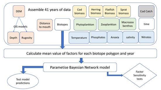
Figure 2.
Flow model of Bayesian network development. The spatial data (rounded boxes) were first checked for quality across 41 years. The data were then aggregated based on the biotope polygons for every year. The BN was then parameterized from this large dataset. The model was subsequently used to make predictions with comparison to the actual observations (oval shape). The factors that make up the model were assessed in terms of sensitivity in order to understand the model influences (diamond shape).
2.3. Development and Application of the BN Model
The development and application of the BN model consists of six phases:
- Causal diagram design resulting in the network structure;
- Variables present in the model;
- Parametrization of the BN from observational data;
- Model testing;
- Scale and non-stationary nature of the BN cod biomass;
- Prediction of cod biomass for biotope for each time period.
2.4. Causal Diagram Design and Bayesian Network Construction
The first step was to construct a diagram of the key environmental correlates and other variables that influenced the species of interest. In this regard, we used expert opinion from the authors and INSPIRE (https://www.bonus-inspire.org/ accessed on 10 January 2022) project partners combined with influences from the literature. The guiding principles regarding which variables to include were the relevance to the ecological dynamics, the state of the data quality, the spatial coverage, and the temporal integrity over the period 1974 to 2014. The causal diagram was assembled with 24 variables and 55 linkages, with an essentially bottom-up perspective on cod biomass (Figure 3). The casual diagram has five major components reflecting the key influences on cod biomass. The structural nodes (grey nodes in Figure 3) do not alter over time, but provide a foundation for the benthic and environmental interactions. The environmental nodes (blue nodes in Figure 3) critically influence the lower trophic components. The plankton nodes capture a selected set of phytoplankton and zooplankton that are influenced by the environmental conditions [33]. The macrozoobenthos node was a combined selection of smaller benthic organisms that are likely to be eaten by cod; this selection was based on the analysis of cod stomach data [34]. The final group was the fish biomass in both the benthic and pelagic zones for cod, sprat, herring, and flatfish (primarily flounder and plaice). Included in the fish group were the cod catch estimates. Attempts were made to include additional variables at the “top end” of the trophic scale [35], including sea bird abundances, seal abundances, and fishing fleet sizes, but these variables had too many gaps across the time period. Linkages between the variables (nodes) are based on expected causal influences extracted from the literature. This diagram then becomes a causal network and the foundation for the expert opinion for the project. Finally, the causal network was developed into a BN by converting each node to a set of discrete states.
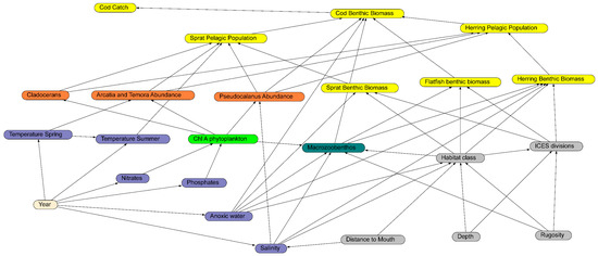
Figure 3.
The completed BN with boxes and arrows showing the parameters and dependencies included. The box colors highlight the structural (grey), environmental (purple), phytoplankton (light green), zooplankton (orange), macrozoobenthos (brown), fish (yellow), and time (beige) components. Each arrow represents a modelled conditional probability element. The data that underpin each node in the BN are described above.
2.5. Variables Present in the Model
The following is a description of the variables or nodes (bold text with shorthand denotations used in figures) present in the model. Cod catch (CC) shows the commercial catch by ICES subdivision 1974 to 2013 [36,37], with equal-frequency bins based on abundance in millions. Cod benthic biomass (CB) was based on scientific bottom trawl data from 1974 to 2014 [38], with equal-frequency bins, and based on biomass calculated from length and abundance data N*W = a*L^b, where a = 0.0079 and b = 3.05. Herring pelagic biomass (HA) was based on acoustic surveys verified by catch data and extrapolated to the ICES rectangles between 1984 and 2014 [36,37], as well as older data [39]; the bins were equal frequency, and the biomass was calculated from length and abundance data N*W = a*L^b, where a = 0.0069 and b = 3.04. Sprat pelagic biomass (SpA) was based on acoustic surveys verified by catch data and extrapolated to the ICES rectangles from 1984 to 2014 [36,37], as well as older data [39]; the bins were equal frequency, and the biomass was calculated from length and abundance data N*W = a*L^b, where a = 0.0055 and b = 3.06. Herring benthic biomass (HB) was based on bottom trawl data from 1974 to 2014 [38]; the bins were equal frequency, and the biomass was calculated from length and abundance data N*W = a*L^b, where a = 0.0069 and b = 3.04. Flatfish benthic biomass (FF) was based on bottom trawl data combined for flounder and plaice from 1974 to 2014 [38]; the bins were equal frequency, and the biomass was calculated from length and abundance data N*W = a*L^b, where a = 0.0093 and b = 3.05 (flounder) and a = 0.0093 and b = 3.03 (plaice). Sprat benthic biomass (SpB) was based on bottom trawl data from 1974 to 2014 [38], with equal-frequency bins, and biomass calculated from length and abundance data N*W = a*L^b, where a = 0.0055 and b = 3.06. Cladocerans abundance (CL), Acartia and Temora abundance (AT), and Pseudocalanus abundance (psu) were based on multi-depth tow samples of plankton collected by the Finnish Institute of Marine Research (1979–2008) and the Finnish Environment Institute Marine Research Centre (2009+) from 1979 to 2013; these data were retrieved from the Global Plankton Database, NOAA [40], with the assistance of Maiju Lehtiniemi, the manager of the collection; the bins were equal frequency, and showed the abundance per volume. Macrozoobenthos (BG) was based on benthic grab data and filtered for species relevant to cod consumption from 1974 to 2007 by MarBEF [41]; the bins were equal frequency for the abundance data. Chl A phytoplankton (CHL) was based on in situ samples from 1974 to 2009 and stored in the Baltic Nest data [42,43]; the bins were split into the following groups: 0 to 1, 1 to 2, and 2 to 9.5, in units of chlorophyll (µg/L). Spring temperature (TSp) was based on in situ samples averaged for the depths 0 to 40 m for the months March, April, and May from 1974 to 2009 and stored in the Baltic Nest data [42,43]; the bins were equal frequency, in units of degrees Celsius. Similarly, the summer temperature (TSu) was based on in situ samples averaged for the depths 0 to 20 m for the months June, July, and August from 1974 to 2009, and also stored in the Baltic Nest data [42,43], with equal-frequency bins and in units of degrees Celsius. Nitrates (no3) were based on in situ samples collected in January and February from 1974 to 2009 and stored in the Baltic Nest data [42,43]; the bins were split as follows: 0 to 2, 2 to 5, and 5 to 22, in units of µmol/L. Phosphates (po4) were based on in situ samples collected in January and February from 1974 to 2009 and stored in the Baltic Nest data [42,43]; the bins were split as follows: 0 to 1, 1 to 1.5, and 1.5 to 4, in units of µmol/L. Salinity (sal) was based on in situ samples restricted to 10–50 m from 1974 to 2009 and stored in the Baltic Nest data [42,43]; the bins were split as follows: 0 to 7.5 and 7.5 to 34, in units of psu, as described in [44]. Anoxic water (anox) was based on in situ samples restricted to 20 m from the sea floor from 1974 to 2009 and stored in the Baltic Nest data [42,43]; the bins were split as follows: −2 to 6 and 6 to 11, in units of total oxygen mL/L. Habitat class (Hab) was derived from modelled habit based on bathymetry, halocline, substrate, and energy from the EUSeaMap project [32]; the bins were based on grouped classes: shallow muds, shallow sands, shallow coarse or mixed sediments, shallow photic rock or biogenic reef, shallow aphotic rock or biogenic reef, shelf muds, shelf coarse or mixed sediments, shelf rock or biogenic reef, and shelf sands. Distance to mouth (dis) was based on the modelled travel cost from the surface to a point located at 58.0666 N and 9.2666 E (the mouth of the Baltic Sea); the bins were equal frequency, in units of meters from the mouth along a direct path. Depth (Depth) was based on a bathymetry model stored in the Baltic Nest data [42,43], with bins of equal frequency and in units of meters. Rugosity (rug) was based on a neighborhood measure calculated from minimum depth per depth range for 3 × 3 neighborhood pixels; the bins were equal frequency, with units of rugosity measured from 0.24 (low) to 0.74 (high). ICES (International Council for the Exploration of the Sea) divisions (div) are the polygon rectangles based on the published ICES divisions and stored in the ICES data portal [42,43]; the bins were grouped by 2 ICES IDs to reduce bin numbers, and included divisions 22 to 32. Year (Yr) was a time counter of the data collection grouped into 4 periods from 1974 to 2014; the periods include the calendar years 1974–1986, 1986–1993, 1993–2004, and 2004–2014. Each biotope has a unique identification number (ID), but this was not used with the model directly.
As recommended by Marcot et al. [14], the number of bins was minimized for enhanced performance and tractability of the underlying conditional probability tables (CPTs). For nodes where a known threshold exists, such as for salinity (7 psu threshold [33]), the bin classes are adjusted accordingly. The years were grouped to capture the major changes in cod biomass in 4 periods (1974–1986, 1986–1993, 1993–2004, and 2004–2014). Habitat class was maintained as a discrete variable describing 9 grouped habitat types. The 11 ICES subdivisions were numbered sequentially from south to north, and were grouped into 7 continuous classes. Bottom oxygen concentration, salinity, and chlorophyll a were allocated bins based on published thresholds [36]. All other variables were binned to represent equal frequency from the observation files (In the Supplementary Figure S1).
2.6. BN Parametrization from Observational Data
The observational data for the Baltic Sea were assembled from a variety of sources. The primary directive was to obtain a spatial location (point or polygon) of a field-based observation. This included benthic grabs and plankton sampling as well as fish population estimates from acoustic surveys and bottom trawl surveys. Additionally, structural aspects (depth and rugosity) were modelled from a digital elevation model. Extrapolation of the data to extend the coverage was specifically avoided in order to reduce the compound effect of multiple model assemblage. A notable exception was the cod catch estimates that were only available at an ICES subdivision polygon scale. The data were then aggregated at a biotope polygon scale and for each year using the mean of the values within the biotope boundaries.
The BN was developed in the modeling shell Netica (version 6.05, Norsys Systems Corp., Vancouver, BC, Canada). The BN before parametrization was considered naïve, since the conditional probability tables (CPTs) will reflect equal distributions for each bin in every node. In order to update the probabilities in the CPTs, we used the expectation maximization learning algorithm [37] within Netica; this approach updates the CPTs automatically as the observational data are considered case by case. Each case here was essentially a row in a table that identifies the habitat polygon, the year, and any relevant information known about the 23 environmental variables in the model. The complete case file (with missing data included) was 1,177,192 rows with 26 columns depicting every habitat polygon and year combination possible. However given that observational data were commonly represented as spatial points, and we were reluctant to extrapolate this spatially limited set across the Baltic Sea environment using some statistical interpolation technique, there were consequently many cases of missing data (~60%)—especially for small habitat polygons. Figure 4 highlights the pattern of the missing data, reflecting the difficulty in obtaining samples for many of these variables. The 397 observations of the cladocerans were an example of scarce data, as shown by Figure 5, whilst noting that only 42 out of 28,712 biotope polygons were sampled across those years. Within the BN, each observation or case was as directly linked to the biotope polygon as possible without the confounding effects of geospatial extrapolations. Biotopes with insufficient data, as defined by 60% missing, were considered to be outside the scope of this model.
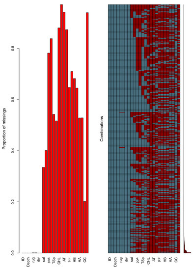
Figure 4.
The graph of the missing data using the aggr function in the VIM R package [38]. The data were a reduced set based on including only cases with at least 14 observations out of a possible 26. The shortened variable names are linked in the data description above.
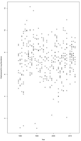
Figure 5.
Graph of the cladoceran observations across the years.
In order to evaluate the model performance using validation, the BN was updated from a naïve state with a random subset of the case file (across all years) containing 70% (81,657) of the cases. The prediction accuracy of the model for the cod biomass node was then tested with the remainder 30% (34,995) of the cases. For every one of the 34,995 cases, the model predicted the likelihood of the cod biomass in each bin, and then compared the prediction directly to the observed value, where it existed for that case within a confusion matrix. An error rate was calculated, meaning that for a percentage of the cases for which the case file supplied a cod biomass value, the network predicted the wrong value. Various other statistical approaches—such as logarithmic loss, quadratic loss, spherical payoff, and area under the receiver operating characteristic (ROC) curve—were calculated [14,39]. Logarithmic loss values (Equation (1) [40]) were calculated using the natural log, and were constrained to 0 and infinity, with 0 indicating the best performance. Quadratic loss (Equation (2) [40]) was restricted between 0 and 2, with 0 being the best, while spherical payoff (Equation (3) [40]) was limited between 0 and 1, with 1 being the best. These measures are defined as follows:
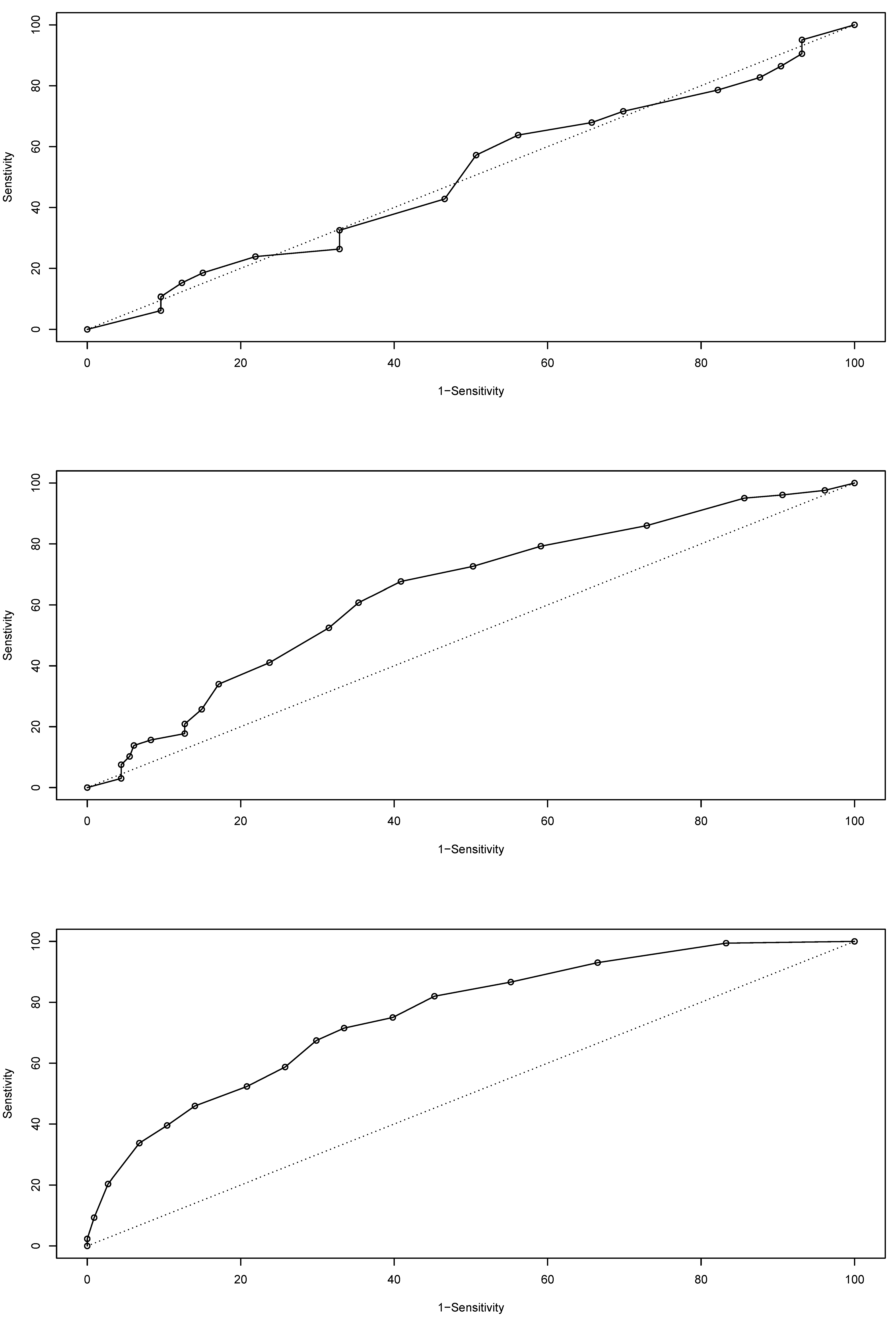
where Pc is the probability predicted for the correct state, pi is the probability predicted for state i, n is the number of states, and MOAC stands for the mean over all cases [40]. Finally receiver operating characteristic (ROC) curves for ICES only, ICES with habitat classes, and ICES with biotopes were generated based on the classification success of the model where the percentage of true positive classification (sensitivity) was greater than the false positives (1 sensitivity) [14,39]. Each point on an ROC curve represents a sensitivity/specificity pair. A model with perfect discrimination between predicted classes has an ROC curve that passes through the upper left corner (100% sensitivity, 100% specificity). Hence, the greater the area under the curve (towards the upper left) relative to the diagonal, the higher the accuracy of the model. Similarly, if the curve goes below the diagonal, the predictions of the model are considered poor discrimination of the classes. The final model was updated with 100% of the cases in order to utilize the full information suite contained in the observational data.
Logarithmic loss = MOAC (−log (Pc))
To examine the predictive capacity of the model, we compared three data profiles:
- Data averaged for each biotope polygon for each year (30% random subset);
- Data averaged for each ICES polygon for each year;
- Data averaged for each habitat class in each ICES polygon for each year.
This provides a way to compare the scale of the data and test the model accuracy. To complete this task the BN model was used to predict the cod biomass based on values where they existed. The cod biomass predictions were compared to the observed values, and the ROC curves were compared.
2.7. Scale and Non-Stationary Nature of the BN Cod Biomass
To address the questions about an effective scale for estimating cod biomass and the value of a non-stationary approach, we focused on the relative influence of each factor in the BN on the cod biomass. The magnitude of changes in cod biomass based on changes in the influencing factors as compared when the spatial unit selected was at the course ICES subdivision scale versus the biotope classification within ICES subdivisions. The changes were measured using a variance reduction technique from the Netica toolbox that produces a table with the magnitude of contribution for each node in the BN [39]. To examine the scale effect, we specified the probability distribution of observing a particular ICES subdivision (i.e., number 28) to be 100% likely, and this then recalculated the marginal probabilities for the remaining BN. The variance reduction calculation was based on this limited probability set and, thus, we were able to estimate the factors that influence the probability distribution given changes in spatial scale (noting that the influences of shape are ignored). Modelling time series based on a stationary stochastic process relies on two assumptions: the independence and identical distribution of the mean and variance of key parameters [41]. If the ecosystem characteristics have changed over time, these assumptions will be violated. In the non-stationary framework, the statistical properties of distributions are specified as a function of different predictors. To examine the effectiveness of adopting a non-stationary approach, we selected two ICES subdivisions and examined the impact of habitat information on the relative influence of significant parameters across the time series. The temporal changes for ICES subdivisions 25 and 28. with and without biotope information, were examined. The nodes with more than 1% influence were recorded. Ideally, the model network topology would also change reflecting the alterations in parameter dependencies, but this would require a machine learning approach to the model’s development.
2.8. Prediction of Cod Biomass per Biotope for Each Time Period
Using the BN model, we predicted the cod and sprat biomass for each period (1974–1986, 1986–1993, 1993–2004, and 2004–2014) and for each biotope polygon based on observed environmental and trophic data, where they existed. The BN model then output an estimate of the probability that a particular cod biomass would be observed for each biotope and for each time period, and this was mapped. This spatially explicit prediction of the cod biomass based on abiotic and biotic factors was a key output of the BN, but other products—such as scenario exploration—are possible.
3. Results
3.1. Model Testing
The isolated 30% case set used to test the model’s capacity to predict Baltic cod biomass showed an overall score of 32.5% error rate for the entire temporal period based on the confusion matrix; it also showed a logarithmic loss value of 0.66, a quadratic loss value of 0.44, and a spherical payoff of 0.75, demonstrating a robust model—especially given the data scarcity. The ROC (Figure 6) shows a high classification success (area under the ROC = 0.7572) of the model. Overall, the model appears robust, with a high degree of prediction capacity—especially when biotope data were included.
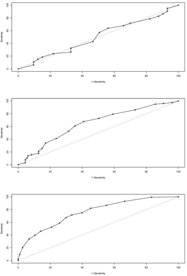
Figure 6.
Receiver operating characteristic (ROC) curves for ICES only (top), ICES with habitat classes (middle) and ICES with biotopes (bottom) [14,39].
3.2. Predictive Changes with Scale
The predictive power of the model altered significantly when habitat information was included, and even more when the unit of analysis was the biotope. The ROC provides a comparison of the prediction of true positives verses false positives for cod biomass (Figure 6). The first dataset, consisting of aggregated ICES subdivisions as the only information (861 cases, 41 years by 21 ICES subdivisions), had a poor predictive capacity (error rate of 64.2%), with an ROC of 0.5015 and the ROC curve dropping below the line of equal distribution separation. This dataset did not contain any benthic biotope information, but did include all the rest where it existed. The next dataset was the 41 years of Baltic data aggregated for the ICES subdivisions partitioned with the biotope classes (5617 cases). This data structure showed an overall error rate of 55.5% and an ROC of 0.6449. As shown in Figure 6, the predictions of the true positives were better than those of the false positives. The final dataset was the aggregated observed data (30% isolated random subset) for each biotope for each year. For this data structure, the error rate was 32.5%, while the ROC was 0.7575. The substantial increase in predictive power was evident across all years when the biotopic data were used to structure the data. In many cases the biotopes crossed the ICES boundaries and had a unique shape.
3.3. Non-Stationary Modelling Based on Selected ICES and Biotope Polygons
To highlight the non-stationary nature of the relationships in the BN model, we closely examined two ICES subdivision polygons (25 and 28, Figure 7) across the time series. The sensitivity of the factors to cod biomass was partitioned into four time periods (Figure 8), and the ICES subdivision 25 with biotope information included (Figure 8, top left) shows an increase in the influence of the factors, particularly with cod biomass. In the last time period—i.e., 2004 to 2014—the sensitivity of the factors decreased. When habitat information was not used to inform the network (Figure 8, top right), there was a steady reduction in sensitivity, with the salinity factor reducing the most. The ICES subdivision 28 showed a constant reduction when no biotope information was included (Figure 8, bottom left); however, the sensitivity of cod catch remained constant across these time periods. When habitat information was included (Figure 8, bottom right), the factor sensitivity magnitude remained constant until the last time period, when macrozoobenthos, flatfish [42], and rugosity emerged as informative (which was likely to be directly related to oxygen stratification [26,43]). Note that the biotope information did not alter during the time series, but the character of the biotope changed as the various environmental factors altered the biotic interactions. This highlights the importance of the model in adjusting the impact of the dependent factors as the other factors change over time.
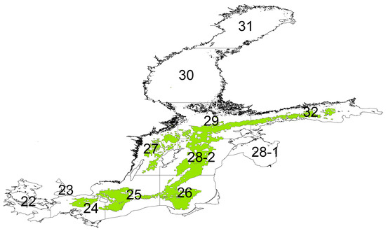
Figure 7.
Spatial map of ICES subdivisions with biotopes that have the shelf mud grouped class type.
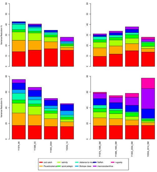
Figure 8.
The magnitude of the dominant influential factors for time periods 1974, 1986, 1993, 2004, and 2014 for ICES 25 (top) and 28 (bottom) without biotope information (left) and with biotope information (right).
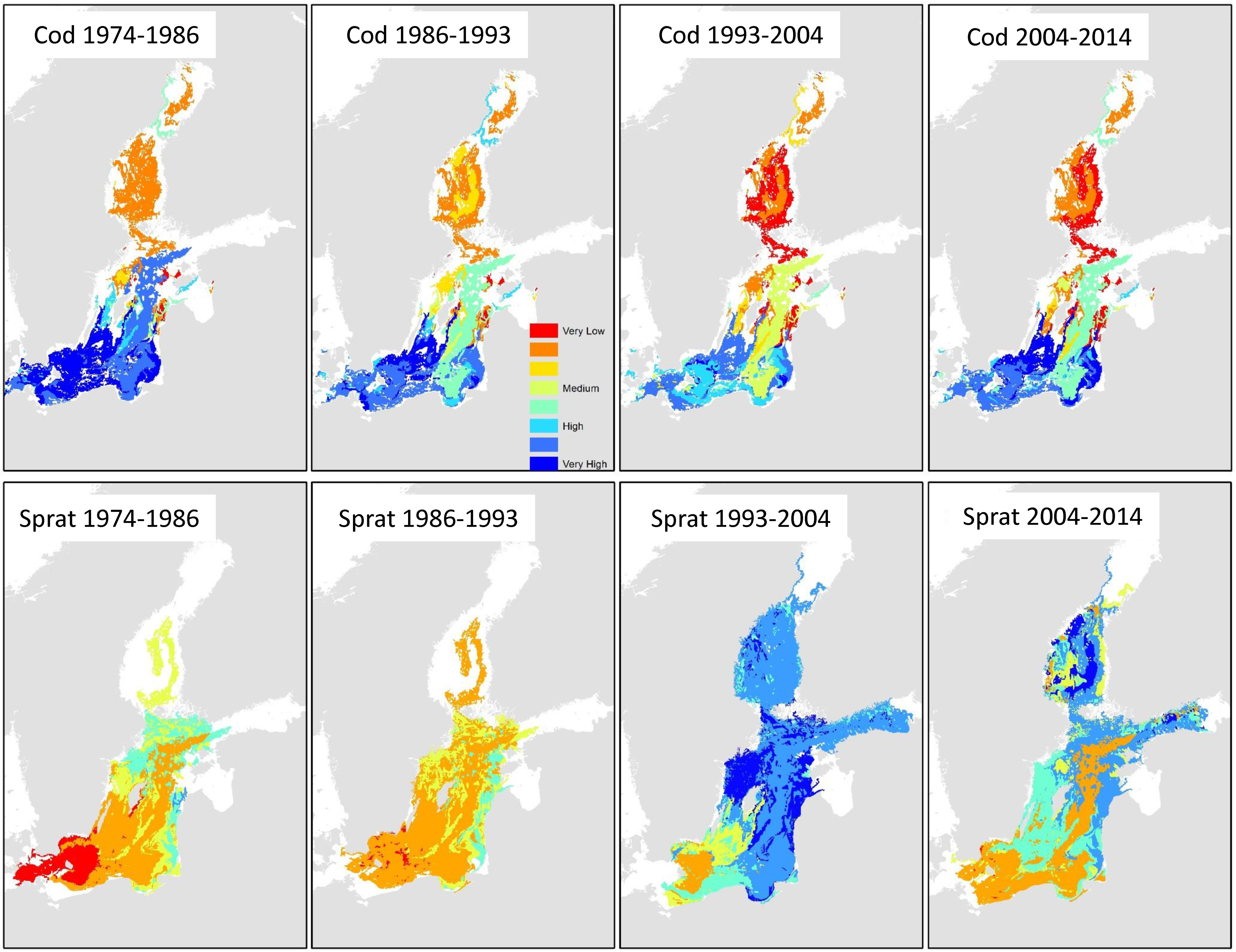
Predictions of the cod spatial distributions can be contrasted with the sprat biomass predictions, as shown in Figure 9. Biotopes with more than 61.5% null data values were excluded from predictions in order to reduce uncertainty. The map composite highlights the changes in the spatial usage of the central and coastal Baltic Sea regions by cod and sprat. In particular, the dominance of the central Baltic region by cod was replaced by sprat dominance in the 1993 to 2004 period. However, in the decade 2004 to 2014, the central region exhibited high uncertainty in the fish population dynamics—especially compared to the western areas.
Figure 9.
Predictions of high cod and sprat biomass in 4 periods. White areas represent biotopes where the level of information for that year group was below the threshold of missing data; consequently, these were excluded from the predictions.
4. Discussion
This use of 41 years of environmental and biotic data within a Bayesian network demonstrates that biotopic information increases predictive capacity for this enclosed region. Understanding the benthic character and incorporating this information into a BN model shows that biotopic conditions are important to developing a spatially explicit and temporally bound model of cod dynamics in the Baltic Sea. Removing this biotopic information or aggregating the model spatial resolution in order to ignore the biotopic boundaries degraded the predictive capacity of the model. In particular, the model was able to accurately predict (within the periods observed) cod biomass across the region, although the predictions for the biotope polygons with insufficient data were discarded. The BN model was not suitable to predict into the future, given the uncertainty of the underlying abiotic and biotic factors, but various future scenarios can be rapidly explored.
Using a variance reduction method to evaluate the contribution of the model factors to the prediction of cod biomass highlighted that trophic, environmental, and biotopic feedbacks—and thus, cod biomasses—were non-stationary. Factors such as macrozoobenthos, flatfish, and rugosity only became influential in the later years of the data, and when environmental factors were different. In contrast, the cod catch factor remained stable in terms of influence, highlighting the fact that while fish catch data were a contributing factor in cod biomass predictions, the model was stationary for this factor. This was despite the substantial decrease in cod catches across this period. A non-stationary approach to a time series is not about the overall changes in a given factor but, rather, the capacity of the time-series model to include the changes in dependencies. Our BN model structure (i.e., the linkages between nodes), however, remained stationary, and there is potential to facilitate the change in network structure as a function of non-stationary changes in correlations observed.
While our model addresses 41 years of observations, it is possible to predict outside this time period (with the addition of extra observational data), and this places extra emphasis on the importance of the non-stationary capacity of the model. Particularly as climate change alters the relationships commonly observed, the inclusion of dynamics in parameter coefficients is required in order to better capture possible future trajectories. However, in agreement with this BN model’s predictions, the recent 2021 ICES advice on fishing opportunities for cod states that catch should be zero in 2022 in order to protect the stock [44,45]. The ICES reports [44,45] continue to note that “The poor status of the eastern Baltic cod is largely driven by biological changes in the stock during the last decades. Growth, condition (weight-at-length), and size-at-maturation have substantially declined. These developments indicate that the stock is distressed and is expected to have reduced reproductive potential”; also important for fisheries management is the statement [44,45] that “Natural mortality has increased and is estimated to be considerably higher than the fishing mortality in recent years”.
The model’s scale was based on the published biotope polygons, and these appear to be a sensible compromise between model size and accuracy. Smaller homogeneous regions could be defined, but the boundary accuracy would demand increased spatial mapping. Models based on a regular raster grid containing fixed cell sizes are restricted in the independence of their observations; either the number of observations is increased (by increasing cell size), or the observations are extrapolated across cells using a selected technique. In either case, the justification for extending the likelihood of occurrence data is problematic, and is isolated from the environmental and ecological associations. Biotopes offer a solution that links ecological processes to benthic structure and, hence, provides a justifiable case for assuming that the observations could have occurred equally within the biotope polygon.
The BN model presented here (Figure 3 and Figure S1) represents one class of model that was employed to understand and predict changes in the biomass of fished species; it is a statistical model, trained on data, and there are numerous examples of different types of statistical models used for similar purposes. For example, to answer similar questions, we could have employed a random forests approach [46]. The strength of the BN approach is that it includes explicit description of the interaction of dependent factors [47]; this was relevant in our study to evaluate the importance of biotopic information that directly affected cod biomass in the Baltic BN. In contrast, the other classes of fisheries/ecosystem models are those that are based on dynamical system representations of food-web interactions and abiotic factors. These models are also well known for their applications in the Baltic Sea, and include large-scale end-to-end models intended to capture the whole-ecosystem dynamics [48,49], models of intermediate complexity that capture the dynamics and strong trophic interactions of only a small subset of species with high detail [50,51,52], and more simple models based on ecological theory such as the size spectra of ecosystems [53,54,55,56]. The important difference between these models and the BN is that the dynamical models often have nonlinear interaction terms. Furthermore, unlike BNs, dynamical models typically do not implicitly account for parameter uncertainty (although parameter sensitivity simulation tests are standard). BNs with discrete bins have linear interaction terms, and it would be interesting to conduct future work to explore whether the nonlinear aspects of dynamical systems models and the parameter uncertainty aspect of BNs could be employed simultaneously.
The selection of the ICES subdivisions for comparison aligned the model evaluation with current fisheries management [44,57]. For instance, in the case of eastern Baltic cod, the management area spans from SD25 to SD29, while for sprat it is even larger, spanning from SD22 to SD32 (Figure 7). These regions are managed based on the advice of scientists, but here we demonstrate that increasing the resolution from subdivisions to biotope polygons significantly increases the predictive capacity. This was especially important when the uncertainty of the observations was high, or when the number of missing data was great. The conclusion in this regard is that the evaluation of stock dynamics and status should reconcile with the spatial scale of the dominant ecological processes, as suggested by the arrangement based on benthic classification.
Fisheries decisions that are based on environmental flows, fish catch statistics, or simple trophic indicators are limited in their management confidence [47]. Including a range of parameters that can characterize the linkage of fish dynamics as a function of overall system characteristics is more likely to generate meaningful advice on fish catch quotas and restrictions. The BN model shown here was able to integrate a wide array of observations while also using the marginal probabilities to assist with predictions, despite missing data.
The BN model does contain a number of assumptions and limitations. The primary limitation is that the BN configuration is assumed to represent the system without being overly complicated. While BNs are generally robust to variations in network structure, the influence on the conditional probabilities is significant, and cannot be ignored. The BN is also based on the observations that occur within the boundaries of the biotopic polygons, and this implies a direct linkage to ecological processes at this scale, as well as a homogeneous character. In some cases, the processes linking one factor to other factors (i.e., pelagic cod partially feeding on macrozoobenthos, which was not included in our model) may not be tightly constrained to benthic structures. An additional limitation is that the model does not include parameters that have inadequate data but may be influential. For example, the role of expanding seal populations or the influence of seabird colonies was recognized [45], but was not incorporated, due to limited data. One limitation of BNs is their incapacity to incorporate feedback loops, such as the population information from previous years [58]. Dynamic BNs can link factors across time periods, but this is only feasible for simple BNs with large numbers of observations. The model presented here was able to make predictions (within the periods specified) without the knowledge of past observations and, despite this limitation, the implicit incorporation of past trends was expected to increase the accuracy of the model.
The BN model’s complexity and resolution were a compromise between data availability and expert opinion on the ecological processes in the Baltic Sea. Some of the nodes—such as flatfish and phytoplankton—were aggregates of the biota in the respective classes, while other classes—such as sprat and herring—were split into benthic and pelagic components. Similarly, the inclusion of some factors while excluding others—particularly environmental categories—remains in the realm of expert opinion. Additionally, the BN’s behavior was improved by adhering to rules of simplicity for bin number and linkage density [14,15]. Future improvements in exploring the model complexity are likely to be fruitful for fisheries management [47].
The approach taken here to evaluate a BN model of the Baltic Sea fisheries demonstrates a clear need to include the benthic influences, and to do so within a modelling framework that is non-stationary and spatially relevant to the ecological process(es) determining the key variables. The understandable nature of the model flow combined with a robust capacity to deal with missing or inaccurate data is attractive for the managers of fisheries in coastal or enclosed waters.
5. Conclusions
Fisheries science has struggled to accurately inform the management of coastal fisheries. We suggest that this is due to the absence of two key factors: benthic coupling, and non-stationary modelling. The role of the benthic environment as expressed by biotope models provides a linkage to the structural components of the marine interaction. The model presented here using a Bayesian network approach was able to integrate the structural, environmental, and biotic components of the system. Critically, the use of biotope information in the form of polygons of variable shape and size, rather than repeated rectangles, increased the ecological linkages within the model, resulting in enhanced predictive capacity. Coastal systems have commonly undergone change during the short and long term; consequently, the nature of variable interactions needed to be dynamic. The BN model can adjust the relationships across the modelled periods and, hence, enable the inclusion of variables that are important only in certain situations. In this regard, we observed the increased influence of the macrozoobenthos, flatfish biomass, and rugosity towards the later period of the 41-year data observation period. Our results strongly suggest that fisheries management that is able to encompass a spatially relevant suite of abiotic and biotic factors is likely to improve sustainable fisheries programs.
Supplementary Materials
The following supporting information can be downloaded at https://www.mdpi.com/article/10.3390/d14020090/s1, Figure S1. The completed BN with colors highlighting the structural (grey), environmental (purple), phytoplankton (light green), zooplankton (orange), macrozoobenthos (brown), fish (yellow), and time (beige) components. Each node (box) shows the discrete bins and marginal probabilities (as numbers and a bar graphic). Each arrow represents a modelled conditional probability element.
Author Contributions
Conceptualization, S.K. and T.B.; methodology, S.K. and T.B.; software, S.K.; validation, S.K., S.N. (Susa Niiranen), J.W. and T.B.; formal analysis, S.K.; investigation, S.K., S.N. (Susa Niiranen) and T.B.; resources, A.O., M.C., S.N. (Stefan Neuenfeldt), V.B. and M.H.; data curation, S.K.; writing—original draft preparation, S.K.; writing—review and editing, S.K., T.B. and S.N. (Susa Niiranen); visualization, S.K.; supervision, T.B.; project administration, T.B.; funding acquisition, T.B. All authors have read and agreed to the published version of the manuscript.
Funding
This work resulted from the Joint Baltic Sea Research and Development Programme (BONUS) project “Integrating spatial processes into ecosystem models for sustainable utilisation of fish resources” (INSPIRE), which were supported by BONUS (Art 185), funded jointly by the European Union, Innovation Fund Denmark, Swedish Research Council Formas, and the Latvian Academy of Science (grant/award number: 2012-60).
Institutional Review Board Statement
Not applicable.
Informed Consent Statement
Not applicable.
Data Availability Statement
The Baltic Environment Database contains the data from this research: http://nest.su.se/bed/. Accessed on 1 July 2015.
Acknowledgments
This work was initiated within the Study Group on Spatial Analysis for the Baltic Sea (SGSPATIAL), 4–6 November 2014, Gothenburg, Sweden.
Conflicts of Interest
The authors declare no conflict of interest.
References
- Van Hoof, L. Fisheries management, the ecosystem approach, regionalisation and the elephants in the room. Mar. Policy 2015, 60, 20–26. [Google Scholar] [CrossRef]
- Levontin, P.; Kulmala, S.; Haapasaari, P.; Kuikka, S. Integration of biological, economic, and sociological knowledge by Bayesian belief networks: The interdisciplinary evaluation of potential management plans for Baltic salmon. ICES J. Mar. Sci. 2011, 68, 632–638. [Google Scholar] [CrossRef] [Green Version]
- Harvey, C.; Cox, S. An ecosystem model of food web and fisheries interactions in the Baltic Sea. J. Mar. Sci. 2003, 3139, 939–950. [Google Scholar] [CrossRef] [Green Version]
- Bauer, B.; Gustafsson, B.G.; Hyytiäinen, K.; Meier, H.E.M.; Müller-Karulis, B.; Saraiva, S.; Tomczak, M.T. Food web and fisheries in the future Baltic Sea. Ambio 2019, 48, 1337–1349. [Google Scholar] [CrossRef] [Green Version]
- Mahévas, S.; Pelletier, D. ISIS-Fish, a generic and spatially explicit simulation tool for evaluating the impact of management measures on fisheries dynamics. Ecol. Modell. 2004, 171, 65–84. [Google Scholar] [CrossRef] [Green Version]
- Pelletier, D.; Mahevas, S. Spatially explicit fisheries simulation models for policy evaluation. Fish Fish. 2005, 6, 307–349. [Google Scholar] [CrossRef] [Green Version]
- Collie, J.S.; Botsford, L.W.; Hastings, A.; Kaplan, I.C.; Largier, J.L.; Livingston, P.A.; Plagányi, É.; Rose, K.A.; Wells, B.K.; Werner, F.E. Ecosystem models for fisheries management: Finding the sweet spot. Fish Fish. 2016, 17, 101–125. [Google Scholar] [CrossRef]
- Lees, K.; Pitois, S.; Scott, C.; Frid, C.; Mackinson, S. Characterizing regime shifts in the marine environment. Fish Fish. 2006, 7, 104–127. [Google Scholar] [CrossRef]
- Hagerman, L.; Josefson, A.B.; Jensen, J.N. Benthic Macrofauna and Demersal Fish. Eutrophication Coast. Mar. Ecosyst. 2013, 52, 155–178. [Google Scholar] [CrossRef]
- Snickars, M.; Gullström, M.; Sundblad, G.; Bergström, U.; Downie, A.-L.; Lindegarth, M.; Mattila, J. Species–environment relationships and potential for distribution modelling in coastal waters. J. Sea Res. 2014, 85, 116–125. [Google Scholar] [CrossRef]
- Griffiths, J.R.; Kadin, M.; Nascimento, F.J.A. The importance of benthic—Pelagic coupling for marine ecosystem functioning in a changing world. Glob. Chang. Biol. 2017, 23, 2179–2196. [Google Scholar] [CrossRef] [PubMed] [Green Version]
- Geritz, S.A.H.; Kisdi, E. On the mechanistic underpinning of discrete-time population models with complex dynamics. J. Theor. Biol. 2004, 228, 261–269. [Google Scholar] [CrossRef] [PubMed]
- Gonzalez-Mirelis, G.; Buhl-Mortensen, P. Modelling benthic habitats and biotopes off the coast of Norway to support spatial management. Ecol. Inform. 2015, 30, 284–292. [Google Scholar] [CrossRef] [Green Version]
- Marcot, B.G.; Steventon, J.D.; Sutherland, G.D.; McCann, R.K. Guidelines for developing and updating Bayesian belief networks applied to ecological modeling and conservation. Can. J. For. Res. 2006, 36, 3063–3074. [Google Scholar] [CrossRef]
- McCann, R.K.; Marcot, B.G.; Ellis, R. Bayesian belief networks: Applications in ecology and natural resource management. Can. J. For. Res. 2006, 36, 3053–3062. [Google Scholar] [CrossRef]
- Borsuk, M.E.; Reichert, P.; Peter, A.; Schager, E.; Burkhardt-Holm, P. Assessing the decline of brown trout (Salmo trutta) in Swiss rivers using a Bayesian probability network. Ecol. Modell. 2006, 192, 224–244. [Google Scholar] [CrossRef]
- Johnson, S.; Mengersen, K. Integrated Bayesian Network Framework For Modeling Complex Ecological Issues. Integr. Environ. Assess. Manag. 2011, 8, 480–490. [Google Scholar] [CrossRef]
- Eklöf, A.; Tang, S.; Allesina, S. Secondary extinctions in food webs: A Bayesian network approach. Methods Ecol. Evol. 2013, 4, 760–770. [Google Scholar] [CrossRef]
- Bartolino, V.; Tian, H.; Bergström, U.; Jounela, P.; Aro, E.; Dieterich, C.; Markus Meier, H.E.; Cardinale, M.; Bland, B.; Casini, M. Spatio-temporal dynamics of a fish predator: Density-dependent and hydrographic effects on baltic sea cod population. PLoS ONE 2017, 12, 1–17. [Google Scholar] [CrossRef]
- Otto, S.A.; Kornilovs, G.; Llope, M.; Möllmann, C. Interactions among density, climate, and food web effects determine long-term life cycle dynamics of a key copepod. Mar. Ecol. Prog. Ser. 2014, 498, 73–84. [Google Scholar] [CrossRef] [Green Version]
- Orio, A.; Bergström, U.; Florin, A.B.; Lehmann, A.; Šics, I.; Casini, M. Spatial contraction of demersal fish populations in a large marine ecosystem. J. Biogeogr. 2019, 46, 633–645. [Google Scholar] [CrossRef]
- Casini, M.; Hjelm, J.; Molinero, J.-C.; Lövgren, J.; Cardinale, M.; Bartolino, V.; Belgrano, A.; Kornilovs, G. Trophic cascades promote threshold-like shifts in pelagic marine ecosystems. Proc. Natl. Acad. Sci. USA 2009, 106, 197–202. [Google Scholar] [CrossRef] [Green Version]
- Möllmann, C.; Diekmann, R.; Müller-Karulis, B.; Kornilovs, G.; Plikshs, M.; Axe, P. Reorganization of a large marine ecosystem due to atmospheric and anthropogenic pressure: A discontinuous regime shift in the Central Baltic Sea. Glob. Chang. Biol. 2009, 15, 1377–1393. [Google Scholar] [CrossRef]
- Eero, M.; Hjelm, J.; Behrens, J.; Buchmann, K.; Cardinale, M.; Casini, M.; Gasyukov, P.; Holmgren, N.; Horbowy, J.; Hussy, K.; et al. Food for Thought Eastern Baltic cod in distress: Biological changes and challenges for stock assessment. ICES J. Mar. Sci. 2015, 72, 2180–2186. [Google Scholar] [CrossRef]
- Kristensen, E.; Delefosse, M.; Quintana, C.O.; Flindt, M.R.; Valdemarsen, T. Influence of benthic macrofauna community shifts on ecosystem functioning in shallow estuaries. Front. Mar. Sci. 2014, 1, 1–14. [Google Scholar] [CrossRef] [Green Version]
- Casini, M.; Hansson, M.; Orio, A.; Limburg, K. Changes in population depth distribution and oxygen stratification are involved in the current low condition of the eastern Baltic Sea cod (Gadus morhua). Biogeosciences 2021, 18, 1321–1331. [Google Scholar] [CrossRef]
- Aarestrup, K.; Økland, F.; Hansen, M.M.; Righton, D.; Gargan, P.; Castonguay, M.; Bernatchez, L.; Howey, P.; Sparholt, H.; Pedersen, M.I.; et al. Oceanic spawning migration of the european eel (anguilla anguilla). Science 2009, 325, 1660. [Google Scholar] [CrossRef]
- Casini, M.; Blenckner, T.; Möllmann, C.; Gårdmark, A.; Lindegren, M.; Llope, M.; Kornilovs, G.; Plikshs, M.; Stenseth, N.C. Predator transitory spillover induces trophic cascades in ecological sinks. Proc. Natl. Acad. Sci. USA 2012, 109, 8185–8189. [Google Scholar] [CrossRef] [Green Version]
- Andersson, A.; Meier, H.E.M.; Ripszam, M.; Rowe, O.; Wikner, J.; Haglund, P.; Eilola, K.; Legrand, C.; Figueroa, D.; Paczkowska, J.; et al. Projected future climate change and Baltic Sea ecosystem management. Ambio 2015, 44, 345–356. [Google Scholar] [CrossRef] [Green Version]
- Wikstrom, S.A.; Daunys, D.; Leinikki, J. A Proposed Biotope Classification System for the Baltic Sea; AquaBiota Water Research: Stockholm, Sweden, 2011. [Google Scholar]
- Österblom, H.; Hansson, S.; Larsson, U.; Hjerne, O. Human-induced trophic cascades and ecological regime shifts in the Baltic Sea. Ecosystems 2007, 877–889. [Google Scholar] [CrossRef]
- Tomczak, M.T.; Heymans, J.J.; Yletyinen, J.; Niiranen, S.; Otto, S.A.; Blenckner, T. Ecological Network Indicators of Ecosystem Status and Change in the Baltic Sea. PLoS ONE 2013, 8, 1–11. [Google Scholar] [CrossRef] [PubMed]
- Neuenfeldt, S.; Bartolino, V.; Orio, A.; Andersen, K.H.; Andersen, N.G.; Niiranen, S.; Bergström, U.; Ustups, D.; Kulatska, N.; Casini, M. Feeding and growth of Atlantic cod (Gadus morhua L.) in the eastern Baltic Sea under environmental change. ICES J. Mar. Sci. 2020, 77, 624–632. [Google Scholar] [CrossRef]
- Tomczak, M.T.; Niiranen, S.; Hjerne, O.; Blenckner, T. Ecosystem flow dynamics in the Baltic Proper-Using a multi-trophic dataset as a basis for food-web modelling. Ecol. Modell. 2012, 230, 123–147. [Google Scholar] [CrossRef]
- Telesh, I.V.; Schubert, H.; Skarlato, S.O. Revisiting Remane’s concept: Evidence for high plankton diversity and a protistan species maximum in the horohalinicum of the Baltic Sea. Mar. Ecol. Prog. Ser. 2011, 421, 1–11. [Google Scholar] [CrossRef] [Green Version]
- Elmgren, R.; Blenckner, T.; Andersson, A. Baltic Sea management: Successes and failures. Ambio 2015, 44, 335–344. [Google Scholar] [CrossRef] [Green Version]
- Spiegelhalter, D.J.; Dawid, A.P.; Lauritzen, S.L.; Cowell, R.G. Bayesian analysis in expert systems. Stat. Sci. 1993, 8, 219–283. [Google Scholar] [CrossRef]
- Templ, M.; Alfons, A.; Filzmoser, P. Exploring incomplete data using visualization techniques. Adv. Data Anal. Classif. 2012, 6, 29–47. [Google Scholar] [CrossRef]
- Marcot, B.G. Metrics for evaluating performance and uncertainty of Bayesian network models. Ecol. Modell. 2012, 230, 50–62. [Google Scholar] [CrossRef]
- Pearl, J. An economic basis for certain methods of evaluating probabilistic forecasts. Int. J. Man. Mach. Stud. 1978, 10, 175–183. [Google Scholar] [CrossRef]
- Hesarkazzazi, S.; Arabzadeh, R.; Hajibabaei, M.; Rauch, W.; Kjeldsen, T.R.; Prosdocimi, I.; Castellarin, A.; Sitzenfrei, R. Stationary vs non-stationary modelling of flood frequency distribution across northwest England. Hydrol. Sci. J. 2021, 66, 729–744. [Google Scholar] [CrossRef]
- Orio, A.; Bergström, U.; Florin, A.B.; Šics, I.; Casini, M. Long-term changes in spatial overlap between interacting cod and flounder in the Baltic Sea. Hydrobiologia 2020, 847, 2541–2553. [Google Scholar] [CrossRef]
- Orio, A.; Heimbrand, Y.; Limburg, K. Deoxygenation impacts on Baltic Sea cod: Dramatic declines in ecosystem services of an iconic keystone predator. Ambio 2021, 1–12. [Google Scholar] [CrossRef]
- ICES. Benchmark Workshop on Baltic Cod Stocks (WKBALTCOD2). ICES Sci. Rep. 2019, 1, 310. [Google Scholar]
- ICES. Cod (Gadus morhua) in subdivisions 24–32, eastern Baltic stock (eastern Baltic Sea). Rep. ICES Advis. Committee 2020, 27, 1–8. [Google Scholar]
- De’ath, G. Boosted trees for ecological modeling and prediction. Ecology 2007, 88, 243–251. [Google Scholar] [CrossRef]
- Uusitalo, L.; Blenckner, T.; Puntila-Dodd, R.; Skyttä, A.; Jernberg, S.; Voss, R.; Müller-Karulis, B.; Tomczak, M.T.; Möllmann, C.; Peltonen, H. Integrating diverse model results into decision support for good environmental status and blue growth. Sci. Total Environ. 2022, 806, 150450. [Google Scholar] [CrossRef]
- Fulton, E.A. Approaches to end-to-end ecosystem models. J. Mar. Syst. 2010, 81, 171–183. [Google Scholar] [CrossRef]
- Bossier, S.; Palacz, A.P.; Nielsen, J.R.; Christensen, A.; Hoff, A.; Maar, M.; Gislason, H.; Bastardie, F.; Gorton, R.; Fulton, E.A. The Baltic sea Atlantis: An integrated end-to-end modelling framework evaluating ecosystem-wide effects of human-induced pressures. PLoS ONE 2018, 13, e0199168. [Google Scholar] [CrossRef] [Green Version]
- Plagányi, É.E.; Punt, A.E.; Hillary, R.; Morello, E.B.; Thébaud, O.; Hutton, T.; Pillans, R.D.; Thorson, J.T.; Fulton, E.A.; Smith, A.D.M.; et al. Multispecies fisheries management and conservation: Tactical applications using models of intermediate complexity. Fish Fish. 2014, 15, 1–22. [Google Scholar] [CrossRef]
- Kulatska, N.; Neuenfeldt, S.; Beier, U.; Elvarsson, B.Þ.; Wennhage, H.; Stefansson, G.; Bartolino, V. Understanding ontogenetic and temporal variability of Eastern Baltic cod diet using a multispecies model and stomach data. Fish. Res. 2019, 211, 338–349. [Google Scholar] [CrossRef]
- Kulatska, N.; Woods, P.J.; Elvarsson, B.Þ.; Bartolino, V. Size-selective competition between cod and pelagic fisheries for prey. ICES J. Mar. Sci. 2021, 78, 1900–1908. [Google Scholar] [CrossRef]
- Carozza, D.A.; Bianchi, D.; Galbraith, E.D. The ecological module of BOATS-1.0: A bioenergetically constrained model of marine upper trophic levels suitable for studies of fisheries and ocean biogeochemistry. Geosci. Model Dev. 2016, 9, 1545–1565. [Google Scholar] [CrossRef] [Green Version]
- Jennings, S.; Mélin, F.; Blanchard, J.L.; Forster, R.M.; Dulvy, N.K.; Wilson, R.W. Global-scale predictions of community and ecosystem properties from simple ecological theory. Proc. Biol. Sci. 2008, 275, 1375–1383. [Google Scholar] [CrossRef] [PubMed] [Green Version]
- Blanchard, J.L.; Dulvy, N.K.; Jennings, S.; Ellis, J.J.R.; Pinnegar, J.K.; Tidd, A.; Kell, L.T. Do climate and fishing influence size-based indicators of Celtic Sea fish community structure? ICES J Mar Sci. ICES J. Mar. Sci. 2005, 62, 405–411. [Google Scholar] [CrossRef]
- Watson, J.R.; Stock, C.A.; Sarmiento, J.L. Exploring the role of movement in determining the global distribution of marine biomass using a coupled hydrodynamic@_ Size-based ecosystem model. Prog. Oceanogr. 2015, 138, 521–532. [Google Scholar] [CrossRef]
- Lee, J.; South, A.B.; Jennings, S. Developing reliable, repeatable, and accessible methods to provide high-resolution estimates of fishing-effort distributions from vessel monitoring system (VMS) data. ICES J. Mar. Sci. 2010, 67, 1260–1271. [Google Scholar] [CrossRef] [Green Version]
- Uusitalo, L. Advantages and challenges of Bayesian networks in environmental modelling. Ecol. Modell. 2007, 203, 312–318. [Google Scholar] [CrossRef]


Publisher’s Note: MDPI stays neutral with regard to jurisdictional claims in published maps and institutional affiliations. |
© 2022 by the authors. Licensee MDPI, Basel, Switzerland. This article is an open access article distributed under the terms and conditions of the Creative Commons Attribution (CC BY) license (https://creativecommons.org/licenses/by/4.0/).