Abstract
The desert ecosystem occupies an important position in the composition of global biodiversity. The Tarim Basin is located in south Xinjiang of China and has the world’s second largest mobile desert, the Taklamakan Desert. As an endemic species in this region, Phrynocephalus forsythii has been demonstrated to have a potentially high extinction risk due to climate change. In order to understand the overall genetic status and provide accordant conservation strategies for the species, we investigated the genetic diversity and population structure of P. forsythii from 15 sites in the Tarim Basin using 21 highly polymorphic microsatellite markers. We found significant genetic structure across the study region. We also revealed generally low levels of gene flow between the 25 sites, suggesting individual dispersal and migration may be restricted within populations. In addition, geographical distance and ambient temperature might be important factors in explaining the observed genetic structure. Our results will provide a scientific basis for the future protection of P. forsythii in this area, as well as an important reference for the conservation and management of biodiversity in desert ecosystems.
1. Introduction
Desert ecosystems are among the most dominant ecosystems and an essential element of the terrestrial landscape [1]. The natural environment of desert ecosystems is exceedingly fragile, and its formation and development are the consequence of arid climate, surface processes, and the evolution of vegetation [2,3]. Desertification is a major issue in arid and semi-arid areas, threatening approximately 41 percent of the world surface area and more than 38 percent of the population [4,5]. Global Desertification Vulnerability Index (GDVI) showed that surrounding regions are at high risk of desertification. Meanwhile, the Representative Concentration Pathways (RCPs) predicted an increased risk of desertification mainly in China and northern India [6,7]. As one of the most widespread ecosystems in China, desert ecosystems are also sensitive to global change [8]. On the other hand, this complex natural environment has nurtured a rich diversity of flora and fauna, and its organisms are unique compared to other ecosystems and occupy an important position in the composition of global biodiversity [9].
The Tarim Basin, located in south Xinjiang Province, is the largest inland basin in China. It nourishes the world’s second largest mobile desert, the Taklimakan Desert [10,11]. The Tarim Basin is 1500 km long from east to west and 600 km wide from north to south, covering an area of about 530,000 km2 and surrounded by altitudes ranging from 800 to 1300 m. It is characterized by a typical arid climate with low precipitation and high evaporation [12]. Due to the extreme harshness of the ecological environment, the process of aridification in the Taklimakan Desert and its climate changes have a significant impact on the population structure of species [13,14]. Currently, research in the Tarim Basin and the hinterland of the desert has mostly focused on plants, especially cherished and endangered plants [15,16], and has concentrated on the evolutionary history and phylogenetic processes [17,18,19]. However, research on the genetic diversity, structure, and differentiation of animal populations in the hinterland and surrounding areas of the Taklimakan Desert is relatively lacking. Zhang et al. (2022) revealed the genetic mechanism of Ovis and environmental adaptability of local sheep breeds in the Taklimakan Desert by analyzing the genome and transcriptome with different agro-geographical characteristics, providing a theoretical basis for the development and conservation of sheep breed germplasm resources in extreme desert environments [20]. The desert and semi-desert inhabited ungulate Gazella subgutturosa has declined sharply due to natural factors and habitat fragmentation. Studies on this species in Xinjiang showed that their population had a low level of genetic diversity, and there was a certain genetic differentiation among the populations, underscoring the urgent need to strengthen the conservation of genetic diversity of G. subgutturosa in Xinjiang [21].
As predominant species in desert ecosystems, reptiles have successfully survived in arid environments by improving morphological and physiological characteristics such as temperature regulation, water balance, and movement processes [22,23]. Phrynocephalus forsythii, belonging to the family Agamidae, is an endemic species of the Tarim Basin and is a viviparous lizard that inhabits sparse scrub or the Gobi area. Research on evolutionary history and phylogeny of P. forsythii is relatively mature [13,24], whereas studies on its genetic structure and population differentiation are still rare.
The amount of genetic diversity reflects the diversity of genetic factors and their combinations that determine biological traits. The richer the genetic diversity, the richer the morphological, behavioral, physiological, and other characteristics of the population and the stronger the adaptability to the environment. Therefore, the amount of genetic diversity can be used as an indicator of population adaptability to its environment [25]. Although P. forsythii was not currently identified as endangered, it was demonstrated with the potential for a high risk of extinction under climate change [26]. Sinervo et al. (2018) developed an eco-physiological model for predicting extinction risk under climate change for 20 Phrynocephalus lizards and revealed 12 of them, including P. forsythii, being at high extinction risk due to exceeded thermal limits. Additionally, by building a climate refugia map using locations of Nature Reserves and extinction areas of China, the author demonstrated that current distribution sites of P. forsythii were beyond the refugia map [26]. Baseline genetic data on genetic diversity and structure, therefore, is crucial for understanding the overall genetic status and providing accordant conservation strategies for the species. Our study specifically aimed to investigate the genetic diversity and population structure of P. forsythii from 15 sites in the Tarim Basin using 21 highly polymorphic microsatellite markers. We also incorporated geography distance data and climatic factors in the analyses to preliminarily infer the potential influence on genetic structure. The results are expected to complement and enrich the basic genetic data of P. forsythii in the Tarim Basin, providing the scientific and theoretical basis for the conservation of the species and contributing an important reference for the conservation and management of biodiversity in desert ecosystems.
2. Materials and Methods
2.1. Study Area and Sample Collection
Based on the reported distribution areas of P. forsythii and our own field observation [27,28], a total of 171 individuals were sampled from 15 sampling sites around the Tarim Basin region (Figure 1; Table 1). After measuring basic data such as body length, tail length, and head length, a piece of tissue (~5 mm2) was cut from the posterior end of the tail, and one toe was also clipped for individual identity. Tissues were preserved in a solution consisting of a volume ratio of 1:1 with anhydrous ethanol and normal saline for subsequent molecular analyses.
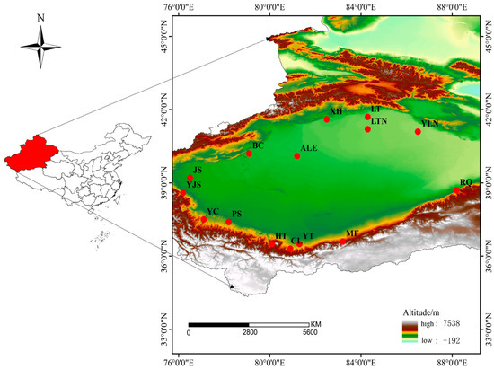
Figure 1.
Map of sampling sites of P. forsythii in the Tarim Basin. Map was edited using data downloaded from the National Foundation Geographic Information System (NFGIS) (https://www.webmap.cn/ (accessed on 16 March 2023)).

Table 1.
Sampling information and genetic diversity parameters.
2.2. DNA Extraction and PCR Amplification
The SteadyPure Universal Genomic DNA Extraction Kit (AGBIO, Changsha, China) was used to extract the whole genome in accordance with the manufacturer’s instructions. Twenty-one highly polymorphic fluorescently labelled microsatellite markers were amplified, including ten (PVMS11, PVMS12, PVMS15, PVMS18, PVMS20, PVMS32, PVMS35, PVMS38, and PVMS39) developed by Zhan and Fu (2009) [29] and eleven (Phr58 excluded) by Urquhart et al. (2005) [30]. PCR amplification was conducted using the MRT (Multiplex-Ready Technology) method [31]. PCR reactions were performed in a 12 µL total volume containing 2.4 μL of 5 × buffer (Mg2+ free), 0.06 μL of 5 U/μL Immolase DNA polymerase, 0.09 μL of 10 μmol/L fluorescently labeled upstream primer tag F (FAM, NED, VIC, PET), 0.09 μL of 10 μmol/L downstream primer tag R, 2.4 μL of 0.4 μmol/L locus-specific primers, 2 μL of template DNA, and the rest was supplemented with ddH2O. Amplification was performed with cycling conditions as follows: pre-denaturation at 95 °C for 10 min; 5 cycles of denaturation at 92 °C for 60 s, annealing at 50 °C for 90 s, and extension at 72 °C for 60 s; 20 cycles of denaturation at 92 °C for 30 s, annealing at 63 °C for 90 s, and extension at 72 °C for 60 s; 40 cycles of denaturation at 92 °C for 15 s, annealing at 54 °C for 30 s, and extension at 72 °C for 30 s; and a final extension at 72 °C for 30 min, preserved at 4 °C. All PCR products were detected by 1.4% agarose gel electrophoresis and sequenced by capillary electrophoresis (GENEWIZ, Suzhou, China).
2.3. Genetics data Processing and Analysis
2.3.1. Genetic Diversity
Sequencing results were scored using GeneMarker® HID [32]. Based on 1000 bootstraps and a 95% confidence interval, the possibility for substantial allele dropout and stuttering was calculated using Micro-checker version 2.2.3 [33]. Hardy–Weinberg equilibrium (HWE) and linkage disequilibrium (LD) among loci were calculated by Genepop version 4.7.5 [34]. Sequential Bonferroni corrections were applied to adjust significance values for multiple comparisons [35]. GenAlEx version 6.51 [36] was used to generate allelic frequencies and to estimate genetic diversity parameters, including effective number of alleles (Ne), observed heterozygosity (Ho), and expected heterozygosity (He). The mean number of alleles per locus (A), inbreeding coefficient (Fis), and allelic richness (AR) for each population were obtained using the R package ‘diveRsity’ (R version 4.2.1) [37,38]. Internal relatedness (IR) was also calculated as an estimate of parental relatedness [39] in an R extension package, Rhh (R version 4.2.1) [38,40]. Fixation index (FST) was used to investigate patterns of differentiation among populations. Calculation of actual differentiation DEST [41] also was performed in an R package ‘DEMEtics’ (R version 4.2.1) [38,42], as FST may underestimate differentiation when using highly polymorphic markers such as microsatellites [41].
2.3.2. Genetic Differentiation and Population Structure
Population genetic structure was evaluated using Bayesian clustering analysis of individual genotypes in various ways. Initially, we implemented the Bayesian genetic clustering algorithm to determine population genetic structure in STRUCTURE version 2.3.4 [43]. We ran the analysis with a burn-in of 10,000 and 300,000 Markov Chain Monte Carlo (MCMC) steps after the burn-in, using an admixture model and correlated allele frequencies without contributing any information on geographic location. The value of K was tested from 1 to 15 due to the possibility of each location representing a distinct genetic cluster, and 10 replicates of each K were run. The best K was determined using STRUCTURE HARVESTER web version 0.6.94 [44], according to the ∆K proposal by Evanno et al. [45]. For the 10 runs of the best K, we used CLUMPP version 1.1.2 [46] to average the membership probabilities, and DISTRUCT 1.1 [47] to visualize the final results.
Discriminant Analysis of Principal Components (DAPC) is another widely used strategy for analyzing the clustering relationships [43,48]. When the level of genetic differentiation is low, it is a multivariate analysis that really is independent of the HWE hypothesis and provides a higher resolution of population structure [48]. We performed DAPC analysis and determined the best clustering K by using R package ‘adegenet’ (R version 4.2.1) [38,49]. The value of K was set from 1 to 15, and 10 replicates were run for each K. Using the Bayesian Information Criterion (BIC) parameter values for each K as reference, the best K was determined by the trend in successive BIC values (BIC decreased sharply to decreased slightly or increased), according to Ward’s hierarchical clustering methods [50]. The number of principal components (PC) used in the DAPC analysis is critical, and the effect of different PC numbers on the results can be considerable. Consequently, cross-validation was employed to determine the best number of PCs to retain explain majority of the sources of variation.
2.3.3. Spatial Scales of Genetic Variation
The correlation between genetic distance and Euclidean geographic distance was evaluated using the Mantel test and Mantel correlogram to determine the impact of geographical distance on genetic differences in the population. The Mantel test was used to determine the effect of isolation by distance (IBD) using GenAlEx 6.51 [36]. Spatial autocorrelation analysis was also performed using 50 km and 100 km distance classes to further study the spatial distribution scale of genetic variation (statistical calculations of spatial autocorrelation were based on 95% confidence intervals defined by 1000 random permutations).
As a complement to the Mantel test, redundancy analysis (RDA) was used to analyze the relationship between genetic structure and explanatory variables. RDA is a multiple linear regression analysis with greater validity than the Mantel test in species–environment relationships with diversity [51]. The allele frequency at each microsatellite locus was used as the response variable in the RDA analysis, and four variables related to distance were used as explanatory variables: geographic coordinates, minimum distance to nearest population (DN), degree of isolation (DI, calculated as the average distance between a population and its three closest neighboring populations), and mean pairwise distance (MPD). The RDA analysis was performed in the “vegan” package of the R (R version 4.2.1) [38,52], with one distance variable as the main explanatory variable and all other distance variables as covariates.
2.3.4. Correlation of Climatic Factors with Genetic Structure
To evaluate the influence of climatic factors on the genetic differences of P. forsythii, we used RDA to analyze the connection between climatic factors and genetic structure. We downloaded climate data from the World Climate Website (WorldClim, https://www.worldclim.org/ accessed on 20 November 2023) and used ArcGIS to extract 19 climatic variables from the 15 sampling sites in the Tarim Basin (Table A1). After screening using the Pearson correlation analysis to exclude highly correlated factors, the chosen climatic factors were employed as explanatory variables, and the allele frequencies of each microsatellite locus were used as response variables for RDA analysis using the R package ‘vegan’ (R version 4.2.1) [38,52].
3. Results
3.1. Genetic Diversity
The micro-checker showed no evidence of scoring errors associated with stuttering, large allele dropout, or null alleles. When 21 microsatellite loci from 15 P. forsythii populations were evaluated individually, 120 HWE results out of 315 detections were still significantly deviated after sequential Bonferroni correction, whereas no deviation was observed for XH, LT, and JS populations. There were 3150 pairwise locus combinations of linkage disequilibrium test, and 78 were found. Except for YJS, BC, XH, LT, and JS, remaining populations had loci that exhibited linkage disequilibrium. However, all pairwise comparison results were not consistent for the 15 populations (no pairing comparison showed linkage disequilibrium for 15 populations simultaneously). These 21 loci were therefore considered as independently segregating loci.
A total of 21 microsatellite loci detected a total of 2179 alleles in 15 populations of P. forsythii. The number of alleles (A) ranged from 30 (XH) to 274 (PS) with an average of 145.267 (Table 1). The observed heterozygosity (Ho) and expected heterozygosity (He) varied from 0.135 (XH) to 0.594 (MF) and from 0.268 (XH) to 0.829 (PS), respectively (Table 1). Inbreeding coefficient (Fis) varied from 0.210 (LT) to 0.819 (XH) with a mean number of 0.421 (Table 1). Allelic richness (AR) varied from 0.810 (XH) to 2.540 (MF), and internal relatedness (IR) varied from 0.344 (XH) to 0.914 (LT) (Table 1).
3.2. Genetic Differentiation and Population Structure
Paired FST values varied from 0 to 0.210, with 78 results of p values being significant after sequential Bonferroni correction (Table 2). Overall, there was a greater genetic divergence between populations (FST < 0.25; Table 2). Paired DEST values ranged from −10.079 (YJS-MF) to 0.788 (XH-PS), with 44 significant values after correction (Table 2). The DEST values were generally higher than FST, as expected (Table 2).
Table 2.
Pairwise FST values (lower triangle) and pairwise DEST values (upper triangle).
Bayesian clustering analysis using STRUCTURE identified four distinct clusters (K = 4, Figure 2) using the ΔK criterion. MF clustered individually as one blue group. CL, YT, and HT populations clustered into one pink group; PS, YC, YJS, and XH groups clustered as one green group; and the rest (BC, RQ, YLN, LT, LTN, ALE, and JS) clustered together as the red group.
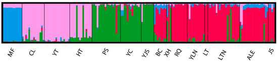
Figure 2.
STRUCTURE clustering diagram.
Cross-validation of DAPC results showed that PC = 26 had the highest percentage of correctly predicted subsamples with the lowest mean square error and was able to explain most of the sources of variation (42.6%). The optimal K value was determined as 5 based on continuous BIC value trends (Figure 3a), and the 15 P. forsythii populations were divided into five groups (Figure 3b). To facilitate comparison of the cluster assignments of the samples at different K values, the posterior probabilities for K values from 2 to 5 were output as bar charts (Figure 3c). The bar chart results indicated that the posterior probabilities of cluster assignment for the samples were all high (97.5%; Figure 3c). The results showed that MF and YT each clustered into one singular group (purple and green, respectively) (Figure 3b,c). ALE, BC, and JS clustered into one pink group, CL and HT clustered into one orange group, and the rest (LT, LTN, PS, RQ, XH, YC, YJS, and YLN) clustered into one dark-green group.
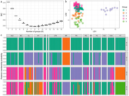
Figure 3.
Results of DAPC showing the genetic structure ((a): Plots showing BIC values with different K; (b): Results of DAPC; (c): Barplots of the posterior probabilities of group assignment for each sample, K = 2–5).
3.3. Spatial Scales of Genetic Variation
Isolation by distance (IBD) analysis showed that the genetic distance (GD) and geographical distance (GGD) of the P. forsythii populations were significantly and positively correlated in the sampling area of the Tarim Basin (R2 = 0.0054, p = 0.021), which indicated that the population was gradually accumulating genetic variation during the dispersal process. Meanwhile, the results of spatial autocorrelation (Figure 4) based on Mantel correlogram demonstrated that the genetic correlation values (r) among individuals in the population at 50 km distance class were significantly negative up to 100 km and positive above 100 km, and r also remained stable around 0 after greater than 100 km (Figure 4a). The results of analyses using a larger distance class of 100 km showed a very similar pattern of correlations to that for the 50 km distance class (Figure 4b).
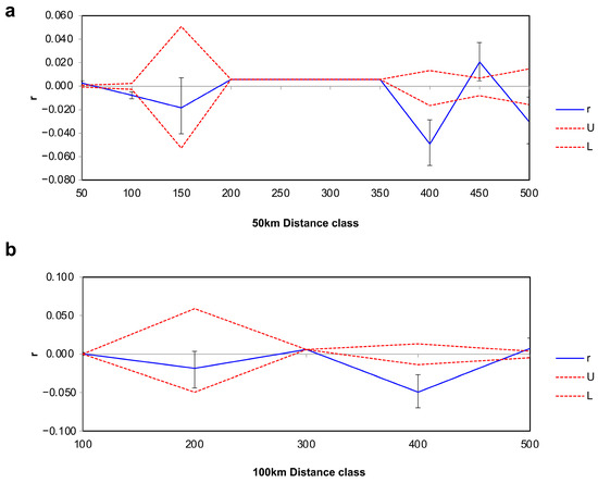
Figure 4.
Correlograms showing genetic correlation (r) as a function of distance ((a): 50 km distance class; (b): 100 km distance). The 95% confidence intervals (dashed lines) were determined by 1000 permutations (U-upper level, L-lower level). Error bars of each estimate of r bounding the 95% confidence intervals were determined by 1000 bootstraps.
RDA analysis with the full model showed a significant correlation between genetic variation and spatial variables (p = 0.006, Bonferroni corrected p = 0.004). The total contribution of the four spatial variables to the genetic variation was 44.1% (13.0% after R2 correction, Figure 5a). Controlling for the effects of the remaining spatial variables (DN, DI, and MPD were used as covariates), RDA analysis with the partial model revealed an explanation of 19.0% (1.5% after R2 correction) when observing the effect of geographic coordinates on genetic variation. The partial full model for the three residual spatial variables (DN, DI, and MPD) showed explanations of 13.2%, 9.2%, and 8.1%, respectively (of 1.3%, 0.4%, and 0.2% after R2 correction, respectively).
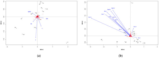
Figure 5.
Triplots of full model RDA analysis: (a) spatial factors; (b) climatic factors. The allele frequencies are displayed in red and the populations are denoted as black open circles. The blue vectors show how explainable variables fall along that RDA space. (x,y) = geographic coordinates; DN = minimum distance to nearest population; DI = degree of isolation; MPD = mean pairwise distance.
3.4. Correlation of Climatic Factors with Genetic Structure
In total, 12 climatic factors were retained (Bio2, Bio4, Bio5, Bio6, Bio8, Bio10, Bio11, Bio13, Bio14, Bio15, Bio16, and Bio17, see Table A1 for full names of the 12 climatic factors) for full model RDA analysis (Figure 5b), and the result showed a non-significant correlation (p = 0.433, Bonferroni-corrected p = 0.432). The 12 climate factors explained 86.2% of the total genetic variation (3.1% after R2 correction), with Bio2 explaining the highest 11.0% (0.3% after R2 correction), followed by Bio15 (5.3%, 0.2% after R2 correction). Results of partial model when the effects of a factor on genetic variation were observed controlling for the remaining climatic variables (with the other 11 climate factors as covariates) are shown in Table A1.
4. Discussion
We used 21 microsatellite loci in the current study to investigate genetic structure and level of gene flow of the P. forsythii in the Tarim Basin region. We found significant genetic structure across the study region, with roughly consistent results from STRUCTURE and DAPC. Along with the results from IBD and RDA analyses, our study revealed generally low levels of gene flow in the study area, suggesting individual dispersal and migration may be restricted to within populations.
The results of HWE test showed that 120 tests deviated from HWE after Bonferroni correction, and no deviation was found in populations with small sample sizes (XH, LT, and JS). The HWE deviation mainly came from populations with relatively large sample sizes, which suggested that the effectiveness of HWE test had limited validity in populations with small samples. Similarly, the small sample size could be also the reason why the XH and LT populations showed significant differences in He. Micro-checker results demonstrated that there were no null alleles in the dataset. Therefore, the HWE deviation is likely to be caused by the Wahlund effect, with causal factors including inbreeding and possible genetic structure.
Regarding the genetic mechanism of inbreeding decline, researchers tend to support the dominant effect theory, which suggests that some recessive pure homozygotes have deleterious effects, and inbreeding increases the proportion of these harmful homozygotes, which will cause the phenotypic performances to exhibit a decrease [53]. The inbreeding coefficient was calculated based on HWE and reflected the relationship between Ho and He. Our Fis results showed that the inbreeding coefficients of 15 populations were higher than 0, indicating that there was a lack of heterozygotes in the population, which was consistent with the results of heterozygous defects in HWE detection, suggesting that the populations may be in the state of inbreeding depression [54]. Negative and a value closer to −1.0 of IR means that there are fewer inbred individuals and less inbreeding in the population, whereas positive and closer to +1.0 means more close relatives and higher inbreeding [55]. The results showed that IR was high (mean of 0.543) and there was no significant difference between populations, suggesting inbreeding may be present in various populations. On the other hand, genetic structure is also a driver of the Wahlund effect. In contrast to inbreeding, individuals in various groups within a large population with genetic structure are more likely to mate with unrelated individuals. If genetic structure is a major factor of the Wahlund effect, then the high Fis and IR in our study cannot be explained by inbreeding. In fact, high Fis values not relating to inbreeding have also been reported in other species [56,57]. Presumably, therefore, high Fis and IR values in our study are likely the reflection of individual mating in a natural state of the species in the study region. This speculation, of course, needs further verification using P. forsythii populations across its whole distribution.
Genetic differentiation index is an important indicator of the degree of genetic differentiation among populations [58]. The greater the degree of differentiation, the more pronounced the genetic structure of the population. FST and DEST of the 15 populations indicated that there were evident genetic differences among the populations, and the differences were mainly from ALE. The pairing comparison between this population and other populations was almost always significant, and the results showed consistency. The LT population was discovered as the least distinct from the other 14 populations, possibly due to its small sample size. Both the IBD test and the RDA analysis of the four distance-related variables and the genetic variation in the population indicated that there was a significant isolation effect of distance in the study area, and geographical distance was significantly and positively correlated with genetic distance within 100 km. Therefore, it is suggested that the population gradually accumulates genetic variation during the process of dispersal. In addition, the dispersal ability of P. forsythii cannot be neglected when considering the geographical isolation effect. Based on previous studies on the relationship between genetic structure and dispersal in vertebrates, it is generally assumed that geographical factors limit species dispersal and thus limit gene flow [59]. The dispersal capabilities of P. forsythii might be crucial to explain the observed genetic structure. At present, however, detailed knowledge on the dispersal distance and home range of the species is still lacking. Further research needs to confirm the threshold dispersal distance and whether the species are capable of fulfilling long-distance movement.
Although the results of the RDA permutation test were non-significant, the mean daily temperature difference (Bio2) was higher than the rest climate factors, suggesting that environmental temperature changes may have a relatively larger effect on the population genetic variation. Evidently, changes in ambient temperature have a regulatory impact on behavior of poikilothermy. Studies have shown that climate warming increases the number of times that poikilothermic animals shuttle between moving into sunlight and drilling into caves to regulate body temperature, which results in shorter predation times, reduced chances of mating, and increased probability of being preyed on by predators, leading to increasing maternal mortality and reducing reproductive output [60,61]. These behavioral regulations may result in decreased effective mating and possibly reduced gene flow. Qi et al. [62] also found a relatively low genetic diversity of P. forsythii in the same region and suggested the high temperature being the main reason. However, detailed studies are needed to confirm the impact of temperature on the genetic variation observed in our dataset.
5. Conclusions
In our study, P. forsythii have some degree of genetic differentiation, with low levels of gene flow between populations, and individual dispersal and migration are largely restricted to within populations, showing a clear genetic structure overall. Geographical distance and environmental temperature may also be important factors affecting the observed genetic structure. Considering its potential extinction risk, we call for strengthening conservations of P. forsythii. Construction of reserves in the Tarim Basin, for example, would be an effective strategy for its protection.
Author Contributions
Conceptualization, Y.L. and P.G.; methodology, Y.L., W.Z. (Wei Zhao) and Y.Q.; validation, Y.L.; formal analysis, J.D.; investigation, L.J., T.C. and W.Z. (Wen Zhong); resources, Y.L.; writing—original draft preparation, J.D.; writing—review and editing, J.D., J.N. and Y.L.; data curation, J.N.; supervision, Y.L.; funding acquisition, Y.L. and P.G. All authors have read and agreed to the published version of the manuscript.
Funding
This research was funded by the National Natural Science Foundation of China, grant No. 32060311; the Gansu Provincial Science and Technology Plan Project, grant No. 20JR10RA124 and 23CXNA0045; the Gansu Province Higher Education Youth Doctoral Support Project, grant No. 2023QB-002; Longyuan Youth Innovation and Entrepreneurship Talent Project of Gansu Province, grant No. 202117; and the Fundamental Research Funds for the Central Universities of Northwest Minzu University, grant No. 31920210143, 31920190083, and 31920230027.
Institutional Review Board Statement
The animal study protocol was approved by the Experimental Animal Ethics Committee of Northwest Minzu University (Approval No.: xbmu-sm-2018050). It was approved on 12 November 2018 and the term of validity is from 1 September 2018 to 31 December 2024.
Data Availability Statement
The data presented in this study are available in a publicly accessible repository (Figshare, DOI: 10.6084/m9.figshare.23700189.v1).
Conflicts of Interest
The authors declare no conflict of interest.
Appendix A
Table A1.
Results for partial models of twelve climatic environmental factors.
Table A1.
Results for partial models of twelve climatic environmental factors.
| Code | Climatic Environmental Factor | Variance Explained | |
|---|---|---|---|
| Variance/% | R2 Corrected Variance/% | ||
| BIO2 | Mean Diurnal Range (Mean of monthly (max temp − min temp)) | 7.4 | 0.2 |
| BIO4 | Temperature Seasonality (standard deviation × 100) | 6.6 | 0.1 |
| BIO5 | Max Temperature of Warmest Month (°C) | 8.8 | 0.8 |
| BIO6 | Min Temperature of Coldest Month (°C) | 8.7 | 0.7 |
| BIO8 | Mean Temperature of Wettest Quarter (°C) | 8.3 | 0.6 |
| BIO10 | Mean Temperature of Warmest Quarter (°C) | 6.4 | 0.2 |
| BIO11 | Mean Temperature of Coldest Quarter (°C) | 6.2 | 0.2 |
| BIO13 | Precipitation of Wettest Month (mm) | 8.2 | 0.5 |
| BIO14 | Precipitation of Driest Month (mm) | 12.6 | 3.3 |
| BIO15 | Precipitation Seasonality (Coefficient of Variation) | 9.8 | 1.3 |
| BIO16 | Precipitation of Wettest Quarter (mm) | 6.4 | 0.2 |
| BIO17 | Precipitation of Driest Quarter (mm) | 10.4 | 1.7 |
References
- Wang, X.; Geng, X.; Liu, B.; Cai, D.; Li, D.; Xiao, F.; Zhu, B.; Hua, T.; Lu, R.; Liu, F. Desert ecosystems in China: Past, present, and future. Earth-Sci. Rev. 2022, 234, 104206. [Google Scholar] [CrossRef]
- Bachelet, D.; Ferschweiler, K.; Sheehan, T.; Strittholt, J. Climate change effects on southern California deserts. J. Arid Environ. 2016, 127, 17–29. [Google Scholar] [CrossRef]
- Iknayan, K.J.; Beissinger, S.R. Collapse of a desert bird community over the past century driven by climate change. Proc. Natl. Acad. Sci. USA 2018, 115, 8597–8602. [Google Scholar] [CrossRef] [PubMed]
- Moran, E.; Ojima, D.; Buchmann, B.; Canadell, J.G.; Coomes, O.; Graumlich, L.; Jackson, R.; Jaramillo, V.; Lavorel, S.; Leadley, P. Science Plan and Implementation Strategy; IGBP Secretariat: Stockholm, Sweden, 2005. [Google Scholar]
- Huang, J.; Li, Y.; Fu, C.; Chen, F.; Fu, Q.; Dai, A.; Shinoda, M.; Ma, Z.; Guo, W.; Li, Z.; et al. Dryland climate change: Recent progress and challenges. Rev. Geophys. 2017, 55, 719–778. [Google Scholar] [CrossRef]
- Feng, Q.; Ma, H.; Jiang, X.; Wang, X.; Cao, S. What has caused desertification in China? Sci. Rep. 2015, 5, 15998. [Google Scholar] [CrossRef] [PubMed]
- Huang, J.; Zhang, G.; Zhang, Y.; Guan, X.; Wei, Y.; Guo, R. Global desertification vulnerability to climate change and human activities. Land Degrad. Dev. 2020, 31, 1380–1391. [Google Scholar] [CrossRef]
- Chen, F.; Chen, J.; Huang, W.; Chen, S.; Huang, X.; Jin, L.; Jia, J.; Zhang, X.; An, C.; Zhang, J.; et al. Westerlies Asia and monsoonal Asia: Spatiotemporal differences in climate change and possible mechanisms on decadal to sub-orbital timescales. Earth-Sci. Rev. 2019, 192, 337–354. [Google Scholar] [CrossRef]
- Whitford, W.G. Desertification and animal biodiversity in the desert grasslands of North America. J. Arid Environ. 1997, 37, 709–720. [Google Scholar] [CrossRef]
- Honda, M.; Shimizu, H. Geochemical, mineralogical and sedimentological studies on the Taklimakan Desert sands. Sedimentology 1998, 45, 1125–1143. [Google Scholar] [CrossRef]
- Sun, J.M.; Liu, T.S. The age of the Taklimakan Desert. Science 2006, 312, 1621. [Google Scholar] [CrossRef]
- Hao, X.; Li, W. Oasis cold island effect and its influence on air temperature: A case study of Tarim Basin, Northwest China. J. Arid Land 2015, 8, 172–183. [Google Scholar] [CrossRef]
- Zhang, Q.; Xia, L.; He, J.; Wu, Y.; Fu, J.; Yang, Q. Comparison of phylogeographic structure and population history of two Phrynocephalus species in the Tarim Basin and adjacent areas. Mol. Phylogenet. Evol. 2010, 57, 1091–1104. [Google Scholar] [CrossRef] [PubMed]
- Shan, W.; Liu, J.; Yu, L.; Robert, W.M.; Mahmut, H.; Zhang, Y. Genetic consequences of postglacial colonization by the endemic Yarkand hare (Lepus yarkandensis) of the arid Tarim Basin. Chin. Sci. Bull. 2011, 56, 1370–1382. [Google Scholar] [CrossRef]
- Borokini, I.T.; Klingler, K.B.; Peacock, M.M. Life in the desert: The impact of geographic and environmental gradients on genetic diversity and population structure of Ivesia webberi. Ecol. Evol. 2021, 11, 17537–17556. [Google Scholar] [CrossRef] [PubMed]
- Gai, Z.; Zhai, J.; Chen, X.; Jiao, P.; Zhang, S.; Sun, J.; Qin, R.; Liu, H.; Wu, Z.; Li, Z. Phylogeography reveals geographic and environmental factors driving genetic differentiation of Populus sect. Turanga in Northwest China. Front. Plant Sci. 2021, 12, 705083. [Google Scholar] [CrossRef] [PubMed]
- Yisilam, G.; Wang, C.X.; Xia, M.Q.; Comes, H.P.; Li, P.; Li, J.; Tian, X.M. Phylogeography and population genetics analyses reveal evolutionary history of the desert resource plant Lycium ruthenicum (Solanaceae). Front. Plant Sci. 2022, 13, 915526. [Google Scholar] [CrossRef] [PubMed]
- Kumar, B.; Cheng, J.; Ge, D.; Xia, L.; Yang, Q. Phylogeography and ecological niche modeling unravel the evolutionary history of the Yarkand hare, Lepus yarkandensis (Mammalia: Leporidae), through the Quaternary. BMC Evol. Biol. 2019, 19, 113. [Google Scholar] [CrossRef]
- Shirazinejad, M.P.; Aliabadian, M.; Mirshamsi, O. The evolutionary history of the white wagtail species complex, (Passeriformes: Motacillidae: Motacilla alba). Contrib. Zool. 2019, 88, 257–276. [Google Scholar] [CrossRef]
- Zhang, C.L.; Liu, C.; Zhang, J.; Zheng, L.; Chang, Q.; Cui, Z.; Liu, S. Analysis on the desert adaptability of indigenous sheep in the southern edge of Taklimakan Desert. Sci. Rep. 2022, 12, 12264. [Google Scholar] [CrossRef]
- Ababaikeri, B.; Ning, L.; Eli, S.; Ismayil, Z.; Halik, M. Microsatellite analyses of genetic diversity and population structure of Goitered Gazelle Gazella subgutturosa (Guldenstadt, 1780) (Artiodactyla: Bovidae) in Xinjiang, China. Acta Zool. Bulg. 2019, 71, 407–416. [Google Scholar]
- Pie, M.R.; Campos, L.L.F.; Meyer, A.L.S.; Duran, A. The evolution of climatic niches in squamate reptiles. Proc. Biol. Sci. 2017, 284, 20170268. [Google Scholar] [CrossRef] [PubMed]
- Bradshaw, S.D. Ecophysiology of Australian arid-zone reptiles. In On the Ecology of Australia’s Arid Zone; Lambers, H., Ed.; Springer International Publishing: Cham, Switzerland, 2018; pp. 133–148. [Google Scholar]
- Qi, Y.; Zhao, W.; Li, Y.; Zhao, Y. Environmental and geological changes in the Tarim Basin promoted the phylogeographic formation of Phrynocephalus forsythii (Squamata: Agamidae). Gene 2021, 768, 145264. [Google Scholar] [CrossRef] [PubMed]
- Humphries, C.J.; Williams, P.H.; Vanewright, R.I. Measuring biodiversity value for conservation. Annu. Rev. Ecol. Syst. 1995, 26, 93–111. [Google Scholar] [CrossRef]
- Sinervo, B.; Miles, D.B.; Wu, Y.; Mendez, D.E.L.A.C.F.R.; Kirchhof, S.; Qi, Y. Climate change, thermal niches, extinction risk and maternal-effect rescue of toad-headed lizards, Phrynocephalus, in thermal extremes of the Arabian Peninsula to the Qinghai-Tibetan Plateau. Integr. Zool. 2018, 13, 450–470. [Google Scholar] [CrossRef] [PubMed]
- Pang, J.F.; Wang, Y.Z.; Zhong, Y.; Hoelzel, A.R.; Papenfuss, T.J.; Zeng, X.M.; Ananjeva, N.B.; Zhang, Y.P. A phylogeny of Chinese species in the genus Phrynocephalus (Agamidae) inferred from mitochondrial DNA sequences. Mol. Phylogenet. Evol. 2003, 27, 398–409. [Google Scholar] [CrossRef]
- Melville, J.; Hale, J.; Mantziou, G.; Ananjeva, N.B.; Milto, K.; Clemann, N. Historical biogeography, phylogenetic relationships and intraspecific diversity of agamid lizards in the Central Asian deserts of Kazakhstan and Uzbekistan. Mol. Phylogenet. Evol. 2009, 53, 99–112. [Google Scholar] [CrossRef]
- Zhan, A.; Fu, J. Microsatellite DNA markers for three toad-headed lizard species (Phrynocephalus vlangalii, P-przewalskii and P-guttatus). Mol. Ecol. Resour. 2009, 9, 535–538. [Google Scholar] [CrossRef]
- Urquhart, J.; Bi, K.; Gozdzik, A.; Fu, J.Z. Isolation and characterization of microsatellite DNA loci in the toad-headed lizards, Phrynocephalus przewalskii complex. Mol. Ecol. Notes 2005, 5, 928–930. [Google Scholar] [CrossRef]
- Hayden, M.J.; Nguyen, T.M.; Waterman, A.; McMichael, G.L.; Chalmers, K.J. Application of multiplex-ready PCR for fluorescence-based SSR genotyping in barley and wheat. Mol. Breed. 2008, 21, 271–281. [Google Scholar] [CrossRef]
- Holland, M.M.; Parson, W. GeneMarker® HID: A reliable software tool for the analysis of forensic STR Data. J. Forensic Sci. 2011, 56, 29–35. [Google Scholar] [CrossRef]
- Van Oosterhout, C.; Hutchinson, W.F.; Wills, D.P.M.; Shipley, P. MICRO-CHECKER: Software for identifying and correcting genotyping errors in microsatellite data. Mol. Ecol. Notes 2004, 4, 535–538. [Google Scholar] [CrossRef]
- Rousset, F. GENEPOP′007:: A complete re-implementation of the GENEPOP software for Windows and Linux. Mol. Ecol. Resour. 2008, 8, 103–106. [Google Scholar] [CrossRef] [PubMed]
- Rice, W.R. Analyzing tables of statistical tests. Evolution 1989, 43, 223–225. [Google Scholar] [CrossRef] [PubMed]
- Peakall, R.; Smouse, P.E. GenAlEx 6.5: Genetic analysis in Excel. Population genetic software for teaching and research-an update. Bioinformatics 2012, 28, 2537–2539. [Google Scholar] [CrossRef] [PubMed]
- Keenan, K.; McGinnity, P.; Cross, T.F.; Crozier, W.W.; Prodoehl, P.A. diveRsity: An R package for the estimation and exploration of population genetics parameters and their associated errors. Methods Ecol. Evol. 2013, 4, 782–788. [Google Scholar] [CrossRef]
- R Core Team. R: A Language and Environment for Statistical Computing; R Foundation for Statistical Computing: Vienna, Austria, 2022; Available online: https://www.R-project.org/ (accessed on 5 May 2023).
- Amos, W.; Wilmer, J.W.; Fullard, K.; Burg, T.M.; Croxall, J.P.; Bloch, D.; Coulson, T. The influence of parental relatedness on reproductive success. Proc. R. Soc. B-Biol. Sci. 2001, 268, 2021–2027. [Google Scholar] [CrossRef] [PubMed]
- Alho, J.S.; Valimaki, K.; Merila, J. Rhh: An R extension for estimating multilocus heterozygosity and heterozygosity-heterozygosity correlation. Mol. Ecol. Resour. 2010, 10, 720–722. [Google Scholar] [CrossRef] [PubMed]
- Jost, L. GST and its relatives do not measure differentiation. Mol. Ecol. 2008, 17, 4015–4026. [Google Scholar] [CrossRef]
- Gerlach, G.; Jueterbock, A.; Kraemer, P.; Deppermann, J.; Harmand, P. Calculations of population differentiation based on GST and D: Forget GST but not all of statistics! Mol. Ecol. 2010, 19, 3845–3852. [Google Scholar] [CrossRef]
- Pritchard, J.K.; Stephens, M.; Donnelly, P. Inference of population structure using multilocus genotype data. Genetics 2000, 155, 945–959. [Google Scholar] [CrossRef]
- Earl, D.A.; vonHoldt, B.M. STRUCTURE HARVESTER: A website and program for visualizing STRUCTURE output and implementing the Evanno method. Conserv. Genet. Resour. 2012, 4, 359–361. [Google Scholar] [CrossRef]
- Evanno, G.; Regnaut, S.; Goudet, J. Detecting the number of clusters of individuals using the software STRUCTURE: A simulation study. Mol. Ecol. 2005, 14, 2611–2620. [Google Scholar] [CrossRef] [PubMed]
- Jakobsson, M.; Rosenberg, N.A. CLUMPP: A cluster matching and permutation program for dealing with label switching and multimodality in analysis of population structure. Bioinformatics 2007, 23, 1801–1806. [Google Scholar] [CrossRef] [PubMed]
- Rosenberg, N.A. DISTRUCT: A program for the graphical display of population structure. Mol. Ecol. Notes 2004, 4, 137–138. [Google Scholar] [CrossRef]
- Jombart, T.; Devillard, S.; Balloux, F. Discriminant analysis of principal components: A new method for the analysis of genetically structured populations. Bmc Genet. 2010, 11, 94. [Google Scholar] [CrossRef]
- Jombart, T. adegenet: A R package for the multivariate analysis of genetic markers. Bioinformatics 2008, 24, 1403–1405. [Google Scholar] [CrossRef]
- Murtagh, F.; Legendre, P. Ward’s hierarchical agglomerative clustering method: Which algorithms implement Ward’s criterion? J. Classif. 2014, 31, 274–295. [Google Scholar] [CrossRef]
- Legendre, P.; Fortin, M.-J. Comparison of the Mantel test and alternative approaches for detecting complex multivariate relationships in the spatial analysis of genetic data. Mol. Ecol. Resour. 2010, 10, 831–844. [Google Scholar] [CrossRef]
- Dixon, P. VEGAN, a package of R functions for community ecology. J. Veg. Sci. 2003, 14, 927–930. [Google Scholar] [CrossRef]
- Makanjuola, B.O.; Maltecca, C.; Miglior, F.; Schenkel, F.S.; Baes, C.F. Effect of recent and ancient inbreeding on production and fertility traits in Canadian Holsteins. BMC Genom. 2020, 21, 605. [Google Scholar] [CrossRef]
- Driscoll, D. Ecological genetics: Design, analysis, and application. Austral. Ecol. 2005, 30, 815–816. [Google Scholar] [CrossRef]
- Pedersen, N.C.; Brucker, L.; Tessier, N.G.; Liu, H.; Penedo, M.C.T.; Hughes, S.; Oberbauer, A.; Sacks, B. The effect of genetic bottlenecks and inbreeding on the incidence of two major autoimmune diseases in standard poodles, sebaceous adenitis and Addison’s disease. Canine Genet. Epidemiol. 2015, 2, 14. [Google Scholar] [CrossRef] [PubMed][Green Version]
- Geiser, C.; Ray, N.; Lehmann, A.; Ursenbacher, S. Unravelling landscape variables with multiple approaches to overcome scarce species knowledge: A landscape genetic study of the slow worm. Conserv. Genet. 2013, 14, 783–794. [Google Scholar] [CrossRef]
- Li, Y.; Lancaster, M.L.; Cooper, S.J.B.; Taylor, A.C.; Carthew, S.M. Population structure and gene flow in the endangered southern brown bandicoot (Isoodon obesulus obesulus) across a fragmented landscape. Conserv. Genet. 2015, 16, 331–345. [Google Scholar] [CrossRef]
- Xu, Y.; Mai, J.-w.; Yu, B.-j.; Hu, H.-x.; Yuan, L.; Jashenko, R.; Ji, R. Study on the genetic differentiation of geographic populations of Calliptamus italicus (Orthoptera: Acrididae) in Sino-Kazakh border areas based on mitochondrial COI and COII genes. J. Econ. Entomol. 2019, 112, 1912–1919. [Google Scholar] [CrossRef] [PubMed]
- Kodandaramaiah, U. Vagility: The neglected component in historical biogeography. Evol. Biol. 2009, 36, 327–335. [Google Scholar] [CrossRef]
- Pincheira-Donoso, D.; Tregenza, T.; Witt, M.J.; Hodgson, D.J. The evolution of viviparity opens opportunities for lizard radiation but drives it into a climatic cul-de-sac. Glob. Ecol. Biogeogr. 2013, 22, 857–867. [Google Scholar] [CrossRef]
- Wang, Y.; Li, S.-R.; Zeng, Z.-G.; Liang, L.; Du, W.-G. Maternal food availability affects offspring performance and survival in a viviparous lizard. Funct. Ecol. 2017, 31, 1950–1956. [Google Scholar] [CrossRef]
- Qi, Y.; Zhao, W.; Huang, Y.; Wang, X.; Zhao, Y. Correlation between climatic factors and genetic diversity of Phrynocephalus forsythii. Asian Herpetol. Res. 2019, 10, 270–275. [Google Scholar] [CrossRef]
Disclaimer/Publisher’s Note: The statements, opinions and data contained in all publications are solely those of the individual author(s) and contributor(s) and not of MDPI and/or the editor(s). MDPI and/or the editor(s) disclaim responsibility for any injury to people or property resulting from any ideas, methods, instructions or products referred to in the content. |
© 2023 by the authors. Licensee MDPI, Basel, Switzerland. This article is an open access article distributed under the terms and conditions of the Creative Commons Attribution (CC BY) license (https://creativecommons.org/licenses/by/4.0/).