Abstract
Climate warming is expected to drive an upward altitudinal shift of species distributions in mountain areas. In this study, we consider how environmental variables constrain the distribution of freshwater mollusks across elevations based on an extensive survey of the entire Pyrenean range. Results show that several altitude-related variables are significantly relevant for the distribution of all mollusks (i.e., temperature, sediment organic content). Others respond more precisely to some variables: fine substrate proportion increases the probability of finding Pisidium sensu lato (mostly Euglesa species), and the latter, the macrophyte presence, and Ampullaceana balthica. Despite the low acid-neutralizing capacity in many of the lakes, only the distribution of A. balthica was significantly constrained by this factor, independent from elevation. The results confirm a likely altitudinal expansion of the distributions of all species, particularly toward lakes with a summer surface temperature increasing above 12 °C. The pace of change is expected to differ among species according to different nonlinear thresholds in thermal response, which temperature value increases from Pisidium s.l. to Ampullaceana to Ancylus, and the taxon-specific sensitivity to substrates and chemical conditions.
1. Introduction
Climate warming drives species distribution shift across the Earth’s thermal gradients [1]. In mountain areas, species are expected to shift their distribution upwards in elevation, with existing examples of plants, birds, and terrestrial insects [2,3,4,5]. Freshwater organisms may delay because of the higher inertia of water due to warming [6]. Distinct life forms may respond differently because of life history and environmental requirements [7]. In the case of mollusks, the carbonaceous shells may represent a particular trait which conditions the response to a warmer climate scenario [8,9,10].
Studies of freshwater mollusk distribution have shown responses to various environmental factors [2,3,4,5]. In the mountains, several considered variables change coherently with elevation, such as temperature, organic matter content, the presence of aquatic vegetation, and the physical nature of benthic substrates [11,12,13,14,15]. Other variables depend more on the bedrock or landcover nature, such as acid neutralizing capacity (ANC) or pH [16,17].
In studies explicitly addressing mountain areas, altitudinal factors [12,18,19] and water chemistry characteristics [16,20,21] have both been found to be significant. Under a warming scenario, the relevance of the two groups of factors for each specific species may result in nonsynchronous responses. Both environmental aspects are relatively independent in mountain areas since water chemistry variation mainly depends on the lithology of lake catchments. Few studies have attempted to explore the relevance of several environmental variables for the distribution of freshwater mollusks [12,15]; particularly, the relative effect of thermal factors and water chemistry gradients on mollusk distributions has not yet been explored in detail in mountain ranges.
In this study, we address the specific context of the entire range of the Pyrenees. Following a previous study comprising all macroinvertebrate groups collected in an extensive survey [22], we selected the most relevant variables for macroinvertebrate groups in general: temperature, sediment organic matter content (LOI), total phosphorus (TP), ANC, the dominance of different substrate types, macrophytes, and fish presence (i.e., Salmonidae). We also included altitude, latitude, and longitude in our statistical approach to explore how mollusks distributions and environmental variables co-vary. While altitude strongly influences many environmental variables, ANC mostly depends on the relative dominance of different lithological units in the catchments, which presents geographically longitudinal biases across the Pyrenees [23,24].
We first explored the coherence of the spatial distribution of mollusks and the selected environmental variables to determine whether there are purely spatial patterns in the distributions, which could suggest dispersal limitations. We then checked for orthogonal latent factors in the constraints imposed by the multivariate environment and whether these factors differentially conditioned some species. Finally, we investigated the probability of occurrence across the relevant environmental gradients identified for each main taxon.
2. Materials and Methods
2.1. Sampling
A survey of 82 mountain lakes in the Pyrenees was carried out during the summer of 2000 (Figure 1). Sampled lakes were selected as a representative subset of the altitudinal and lithological variation of all lakes in the Pyrenees [22]. In the littoral zone, macroinvertebrate samples were collected following the kick-sampling method and a standardized protocol for Nordic lakes [25], using identical sampling effort per lake (i.e., 5 min person). Sampling sites at each lake were selected to represent the habitat variability of the whole littoral, which was explored through a previous inspection of the entire lake perimeter. All macroinvertebrate samples collected at each lake were amalgamated into a unique sample. The benthic substrate variability in the littoral zone was evaluated as the relative cover of several grain-size categories (i.e., fine substrates, stones and gravel, and rocks) and the percentage of macrophyte coverage. Water temperature was measured during the visits, water samples were collected for chemical analyses [24], and catchment characteristics were determined from available GIS information [26,27].
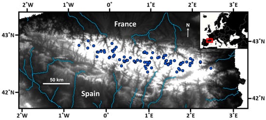
Figure 1.
Distribution of the surveyed lakes across the Pyrenees. The main hydrological structure is highlighted. The white area, where the survey lakes are located, indicates elevations above 1600 m a.s.l. Maps are based on ArcGIS Desktop 9.3 and MapChart (https://www.mapchart.net/).
2.2. Mollusk Sorting and Determination
Macroinvertebrate samples were fixed in 4% formalin in the field and brought to the laboratory for macroinvertebrate sorting under the stereomicroscope. Mollusks collected in each sample were separated and stored in 70% ethanol tubes. The taxonomic determination of mollusks was initially performed at the genus level following general taxonomic references [28,29] and later determined to as much taxonomic resolution as possible, following the more specialized literature (e.g., [30,31,32]).
2.3. Numerical Analysis
The distribution of mollusk taxa was first tested regarding presence/absence as univariate responses to altitude, latitude, and longitude. The three variables followed a normal distribution according to a Shapiro–Wilk test. However, when dividing them into two subsets representing presence and absence, normality was not always achieved in both subsets. For this reason, we opted to compute these univariate relationships with the non-parametric Mann–Whitney test [33]. Abundance patterns concerning altitude, latitude, and longitude were also tested for lakes where a specific mollusk of interest was present, using Spearman correlation tests, because of the high skewness in the number of individuals.
The environmental variability across altitudinal, latitudinal, and longitudinal gradients was tested for each variable individually and then against altitude using a multivariate ordination, a principal component analysis (PCA) incorporating altitude as a passive variable. Variables deviating from normality were log-transformed. Then, we performed a redundancy analysis (RDA) to assess the capability of environmental variables to account for the variance in mollusk data, which were previously transformed to operate with Hellinger distances, following Legendre and Gallagher [34]. Detrended correspondence analysis (DCA) previously showed a relatively short gradient length (1.8 standard deviation units) which discouraged the usage of the canonical correspondence analysis (CCA) instead of the RDA, following Legendre and Legendre [35]. All lakes were used in RDA, regardless of whether mollusks were present, to combine incidence and abundance data in the same multivariate analysis. This approach undoubtedly penalized the total variance explained; however, the main goal was to determine orthogonal latent factors (i.e., main axes) that influence the individual taxa differently. The RDA environmental variables were forward-selected using Monte Carlo tests (9999 permutations). Multivariate analyses were executed with CANOCO v. 4.5 software (Ithaca, NY, USA) [36].
After characterizing the environmental correlations, we investigated the specific univariate responses of mollusks. As a first approach, Mann–Whitney and Spearman correlation tests were used to analyze incidence and abundance patterns, respectively, the latter being analyzed only for lakes where a particular mollusk of interest was present. Non-parametric tests facilitated comparisons since not all environmental variables followed normality. Given its qualitative nature, the exception was Salmonidae, which was analyzed concerning the presence/absence of mollusks with Fisher’s exact tests on a contingency table and with a Mann–Whitney test comparing mollusk data in lakes with and without salmonids [33]. Macrophytes were also re-analyzed as a qualitative variable (presence/absence) concerning the presence/absence and abundance of mollusks, also using the Fisher’s exact test and the Mann–Whitney test, respectively. Finally, we focused on mollusk incidence patterns using binomial generalized linear models (binomial GLMs) to obtain presence probability functions across the relevant environmental gradients. The significance of the slope and intercept of each of these binomial GLMs was estimated. All univariate analyses, including binomial GLMs, were executed in R software [37].
3. Results
3.1. Mollusks Distribution
Mollusks were found in 50 of the 82 lakes sampled, comprising 1279 individuals (Table 1). Sphaeriidae bivalves and the gastropods Ampullaceana balthica and Ancylus fluviatilis were the most frequent taxa found. Species determination of the family Sphaeriidae could only be achieved in 20 out of the 41 lakes where this family was present, mainly due to the small size of many individuals, combined with the effect of the formalin used for preservation on shell shape. The six species determined were from the Euglesa genus (Table 1). However, their individual occurrence was too low for a meaningful ecological study. Therefore, we decided to use Pisidium, sensu lato, for the ecological analyses, pooling undetermined specimens and the six species together, provided that the Euglesa species have been considered until as recently as Pisidium. A few individuals of the gastropods Bythinella and Gyraulus cf. albus were also found. Statistical analyses were performed at the genus level in all frequent mollusks to harmonize comparisons (i.e., Pisidium s.l., Ampullaceana, and Ancylus).

Table 1.
Mollusks found in terms of incidence (number of lake occurrences) and abundance (total number of individuals collected).
Abundance values varied widely, particularly for Ampullaceana and Pisidium s.l., owing to the strong skewness resulting from a high numbers of juveniles in some lakes. For example, up to 297 individuals of Ampullaceana were found in one lake, representing ca. 64% of all individuals found in all lakes (n = 467). Similarly, up to 231 individuals of Pisidium s.l. were accounted for combining only two lakes, representing ca. 37% of all individuals (n = 644). For Ancylus, 57 individuals counted when combining two lakes represented ca. 44% of all individuals (n = 130). Consequently, a numerical analysis of abundance data should be compared cautiously to incidence information.
The occurrence of mollusks was biased toward the lowest elevations. Ampullaceana showed the strongest tendency to inhabit low-altitude lakes. Ancylus showed a lower altitudinal range than Pisidium s.l., but the tendency was not significant, likely due to the low number of occurrences (Figure 2). All species tended to preferentially occur in the eastern part of the range, with Ampullaceana primarily present in the South slope (Figure 3). The abundance patterns were only barely significant (i.e., p 0.03–0.05) for latitude (positive for Ampullaceana, inverse for Pisidium s.l.) and longitude (inverse for Ampullaceana), without a relationship with altitude (Table A1).
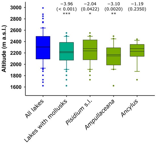
Figure 2.
Altitudinal distribution of mollusk compared to the distribution of the survey lakes. Significance (p-values) refers to Mann–Whitney tests (z-scores) comparing altitude values in lakes with and without the taxon being considered. Asterisks indicate the level of significance: *, p < 0.05; **, p < 0.01; ***, p < 0.001. The mean and median are shown within the boxes; the larger the distance between them, the higher the skewness of the data.
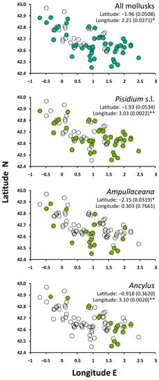
Figure 3.
Spatial distribution of mollusks across the survey lakes. Significance refers to Mann–Whitney tests comparing latitude and longitude values between lakes with (filled circles) and without (empty circles) the taxon of interest. Asterisks indicate the level of significance: *, p < 0.05; **, p < 0.01.
3.2. The Multivariate Environment
All the environmental variables considered showed significant spatial tendencies (Table 2). All variables except ANC and ‘stones and gravel’ showed elevational patterns that were most inversely related to altitude (i.e., temperature, LOI, TP, fine substrate, macrophytes, Salmonidae), yet were positively correlated in the case of rocky benthic substrates. Some variables showed simultaneous correlations to latitude and longitude because of the geographical distribution of lakes in the Pyrenees that follow a Northwest–Southeast alignment (Figure 1 and Figure 3). Longitude primarily encompasses a precipitation gradient related to the predominant Atlantic air masses, and latitude involves the differences between the Northern and the warmer Southern slopes [38]. Temperature, LOI, and fine substrate were positively correlated to longitude, with higher values in the Eastern part, and were inversely correlated to latitude, with higher values in the Southern part. The opposite was observed for ANC and ‘stones and gravel’, responding to a predominance of carbonate bedrock in the Southwestern Pyrenees. The correlation structure between environmental variables (PCA, Figure 4a) reflected the significant influence of the altitudinal gradient. Only ANC and ‘stones and gravel’ were more related to a second axis of variation, independent of altitude.
Table 2.
Relationship between geographical and environmental variables.
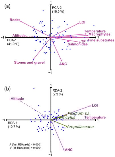
Figure 4.
(a) Principal component analysis (PCA) of the environmental variables considered in the study. (b) Redundancy analysis (RDA) of mollusks distribution (green arrows) with a forward selection of environmental variables. Dashed lines indicate passive variables included in the ordination for comparison with the forward-selected variables. Salmonidae was a nominal variable and, therefore, is indicated as a dot in the biplot.
Due to this strong correlation structure, applying redundancy analysis (RDA) with a forward variable selection to obtain a robust minimum explanatory model resulted in the selection of only one variable representative of each PCA main axes (Figure 4b), LOI, and ANC (Table A2). The overall variance explained by this minimal model was relatively low (12.9%), greatly due to the uneven distribution of the abundances, but also to the restriction imposed by the variable selection procedure, which minimized spurious explanation by false positive, but favored false negative for the variables whereby all of them highly correlated with altitude. Considering the low number of species and their limited occurrence in the lakes, exploring community composition and mollusk relative abundance patterns makes little sense. Relevant distribution details must be elucidated at a single taxa level considering the potentially relevant environmental factors.
3.3. Specific Univariate Responses
Mollusk as a group tended to preferentially occur in warmer lakes, with a higher organic matter content in the sediments, more productivity, and showing less rocky littorals (Table 3). They were rare at summer surface water temperatures below 12 °C and TP < 4 µg L−1, although all species occasionally penetrated these barriers (Figure 5). Due to the high correlation between these variables across the altitudinal gradients, it was more interesting identifying which species depart from the general patterns. Specifically, Ampullaceana did not prefer higher LOI lakes and was unique with a significant correlation with ANC (Table 3). Ancylus did not show a preferential occurrence in more productive lakes, although when considering abundance, showed a significant relationship with TP, which may be spurious, considering the high skewness in abundance values.
Table 3.
Relationship between incidence and abundance of mollusks and environmental variables.
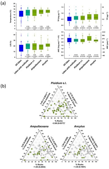
Figure 5.
(a) Temperature, organic content in sediments (LOI), total phosphorus (TP), and acid neutralizing capacity (ANC) distribution according to mollusk taxa compared with all survey lakes. (b) Distribution of Pisidium s.l., Ampullaceana balthica, and Ancylus fluviatilis concerning habitat substrates. Significance (p-values in parenthesis) refers to Mann–Whitney tests (z-scores) comparing values of the variable considered between lakes with and without the taxon of interest. Asterisks denote the level of significance: *, p < 0.05; **, p < 0.01; ***, p < 0.001.
Beyond the physical environment, all species showed significant positive occurrence with macrophytes (Table 3). It could be a false positive because of the preference for similar physical environments by both organisms. However, Fisher’s exact test comparing expected (random mollusk distribution between lakes) and observed frequencies in lakes with macrophytes to have indicated significant mollusk facilitation by macrophytes (Table A3).
The occurrence with fish was also significant, except for Ancylus (Table 3 and Table A3), which also involved an abundance of significance.
Logistic regression models accounting for the presence/absence of the different taxa (binomial GLMs) provided an assessment of the probability of finding a taxon under certain conditions (Table A4), which can be particularly useful for evaluating potential mountain environmental shifts under climate change (Figure 6 and Figure 7). Temperature and LOI significant models were fitted for all species. Additionally, some other models were fitted with low uncertainty to Pisidium s.l. (‘fine substrates’ and ‘stones and gravel’, ‘rocks’, and ‘macrophytes’) and Ampullaceana (ANC, ‘macrophytes’). Concerning temperature, the steepest increase in the probability of the presence of the taxa (higher slopes in Figure 6 plots) occurred at increasing temperatures from Pisidium s.l. (10 °C) and Ampullaceana (12 °C) to Ancylus (14 °C). The same occurred for LOI, Pisidium s.l. (8%), Ampullaceana (18%), and Ancylus (20%). Therefore, shifting to warmer and more organic conditions will particularly favor the expansion of Ampullaceana and Ancylus.
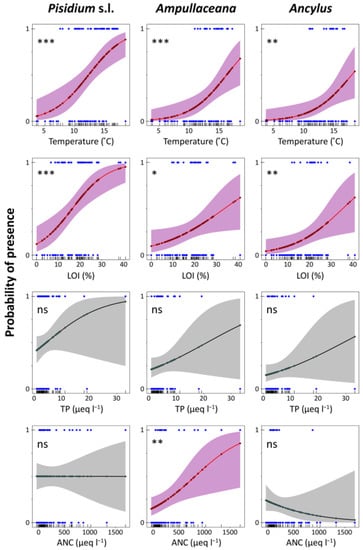
Figure 6.
Logistic regression models for Pisidium s.l., Ampullaceana balthica, and Ancylus fluviatilis concerning temperature, organic content in sediments (LOI), total phosphorus (TP), and acid neutralizing capacity (ANC). Level of significance follows a chi-square test on a deviance table: ns, not significant; *, p < 0.05; **, p < 0.01; ***, p < 0.001.
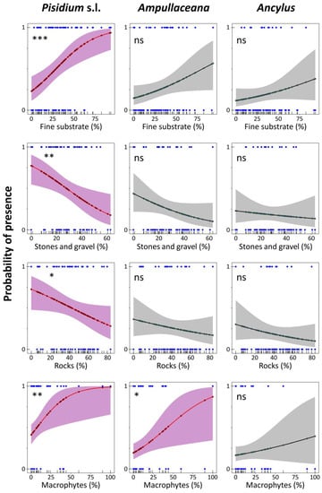
Figure 7.
Logistic regression models for Pisidium s.l., Ampullaceana balthica, and Ancylus fluviatilis concerning habitat substrate dominance and macrophyte coverage. Level of significance follows a chi-square test on a deviance table: ns, not significant; *, p < 0.05; **, p < 0.01; ***, p < 0.001.
Response to substrates was similar for the three taxa (Figure 7), although significant fitting was only achieved for Pisidium s.l. and Ampullaceana and exclusively for macrophyte cover. ‘Fine substrate’ percentage steadily increased the Pisidium s.l. occurrence probability, achieving 80% at about 60% of the ‘fine substrate’. An increased proportion of ‘stones and gravel’ and ‘rocks’ declined the probability. The probability occurrence for Pisidium s.l. without macrophytes was relatively high (40%) and increased steeply, reaching about 80% at 35% macrophyte cover. For Ampullaceana, a similarly high probability required about 75% of macrophyte recovery (Figure 7). Lastly, ANC chiefly increased the presence probability of Ampullaceana, particularly from 500 µeq L−1 (40%) to 1000 µeq L−1 (75%).
4. Discussion
The Pyrenean high mountain mollusk community is relatively poor compared to the lowlands [12,39] as environmental conditions with increasing altitudes deviate from those more suitable to freshwater mollusks. Bivalves are restricted to the genus Pisidium s.l. but include at least six species. Many specimens collected could not be identified at the species level because they corresponded to juveniles. Consequently, the distribution peculiarities of each species could not be investigated because of the lack of sufficient statistical power. In the future, surveys focusing specifically on Pisidium s.l. may disentangle the conditions for the segregation of these species, which have been evaluated here as a single taxon, thus showing a broader distribution than other mollusks considered as single species. Ampullaceana balthica, Ancylus fluviatilis, and the pooled Pisidium s.l. apparently showed some geographical bias across the Pyrenean range. However, the high correlation between the environmental variables that have more influence on mollusk distributions (temperature, LOI, ‘fine substrate’, and ANC) and longitude limits the evaluation of potential geographical patterns. It is worth pointing out that both gastropod species appear at the longitudinal geographical extremes of the Pyrenees; therefore, spatial distribution biases are more likely due to environmental constraints than biogeographical patterns. In altitude, the three taxa analyzed show similar distribution and limits, reflecting that the declining elevational tendency of the environmental conditions are more suitable for them. Indeed, only ANC does not follow such an elevation pattern. Therefore, there are two main axes of variation: one of the variables is related to altitude (i.e., temperature, LOI, and substrate type) and another corresponds to water hardness (i.e., ANC).
4.1. Environmental Constraints Related to Altitude
Several altitude-related variables have a widespread influence on mollusk distributions. Temperature and organic matter content in sediments and a surrogate of lake productivity are the most conspicuous, likely because of a direct beneficial effect on the persistence of all mollusks. Other altitude-related variables, mainly related to the physical nature of benthic habitats, have a more specific influence on specific mollusks, notably the positive influence of fine substrates on Pisidium s.l. and that of macrophytes on Ampullaceana.
The apparent beneficial effect of salmonid presence on mollusk is controversial. It may result from the strong covariation of fish presence and mollusk with altitude. Previous studies found that fish stocking in mountain lakes does not significantly affect the abundance of bivalves [40], whereas trout presence in Arctic Alaskan lakes limits the size of gastropod individuals [41]. A true positive effect could only result from a lower relative fish predation pressure on mollusks than on their competitors [42]. Effects of increased nutrient recycling due to salmonids result in speculation as fish concentration is relatively low in most lakes. Nevertheless, more specific studies are required.
4.2. The Influence of Acid-Neutralizing Capacity
ANC and associated variables (e.g., pH, Ca2+) influence the facility for building carbonate shells; therefore, the low ANC values in many lakes could condition the mollusk establishment. Surprisingly, only the presence of Ampullaceana is favored at higher ANC, whereas the other taxa do not show evident limitation by this factor. Components for shell calcium carbonate formation can either be directly obtained from water or mobilized from other tissues. This latter process has been studied in detail on bivalves [9,43,44]. The process may not be equally efficient in gastropods than bivalves.
Indeed, previous studies indicate that freshwater snails are more prone to be affected by water acidification than bivalves [20,45,46]. The genus Pisidium s.l. appears remarkably tolerant to changes in water acidity [28]. The lowest pH record empirically observed for this genus (i.e., pH = 4.7; [45]) is, in general, lower than that for gastropod species [20,45,46] if some humic lakes are excluded from the comparison [47]. Consequently, gastropods have been considered more valuable organisms than bivalves as indicators of water acidification [21,46,48,49]. According to Brown [8], about 45% of freshwater gastropods are restricted to waters with calcium concentrations >25 mg L−1 and 95% to levels >3 mg L−1.
All in all, within both bivalve and gastropod species, differences in tolerance to water acidity exist [8,28]. Among the gastropods, Lymnaea peregra (=Ampullaceana balthica) has been reported as more sensitive than Ancylus fluviatilis in Northern Europe (Schartau et al., 2008), which agrees with the results obtained in this study. ANC shows a stronger influence on Ampullaceana distribution than on Ancylus. The body size could be a determinant, with Ampullaceana requiring more calcium per individual than the smaller Ancylus. The growth rate in freshwater gastropods is limited in highly diluted waters [50,51,52]. More comparative information about growth rates and calcium physiology between the different mollusk species inhabiting the soft mountain waters will clarify the mechanism underlying the observed patterns.
4.3. Implications in a Shifting Climate Scenario
In the present context of global warming, results from this study justify the expected upward elevational shift in mollusk species distributions. Increased surface summer temperature appears to be a sufficient factor in advancing the altitudinal survival of the species, particularly if the temperature exceeds 12 °C, with bivalves likely at the forefront of the advance as they penetrate colder waters than gastropods. Furthermore, the progressive transformation of the littoral lake conditions with increasing organic matter substrates will enhance the probabilities of colonization, as will occur with macrophytes, since they favor the establishment of Pisidium s.l. and Ampullaceana.
The mollusks that could be expected to be highly restricted by the low water hardness (e.g., low calcium and ANC) common to many high-mountain lakes are already mostly excluded from mountains. For example, most of the European calciphile species listed by Briers [53] are excluded from high elevations in the Alps and the Pyrenees, in contrast to the non-calciphile species listed therein, as evidenced by their distribution maps [54]. From the current communities inhabiting the lakes of the Pyrenees, Ampullaceana will become particularly favored by the intensified weathering rates of lake catchment bedrocks, which result from rising temperatures with consequent ANC increases [55,56]. Local species richness will likely increase because the main species-specific restrictions will soften for more mollusk species, and differential microhabitats use among them may facilitate coexistence. Similarly, current geographical differences will likely diffuse as they appear more related to ecological restrictions than historical biogeographical limits.
Supplementary Materials
The following supporting information can be downloaded at: https://www.mdpi.com/article/10.3390/d15040500/s1, Survey data on mollusk occurrence.
Author Contributions
Conceptualization, G.d.M. and J.C.; methodology, G.d.M., R.A. and J.C.; data-analysis, G.d.M.; data curation, G.d.M. and J.C.; writing—original draft preparation, G.d.M.; writing—review and editing, J.C.; visualization, G.d.M.; supervision, J.C.; project administration, J.C.; funding acquisition, J.C. All authors have read and agreed to the published version of the manuscript.
Funding
This research was funded by European Council, FP5-EESD—grant number EVK1-CT-1999-00032 (EMERGE), and Ministerio de Ciencia e Innovación. Programas Estatales de Generación de Conocimiento y Fortalecimiento Científico y Tecnológico, grant number MCIN/AEI/PID2019-111137GB-C21 (ALKALDIA).
Institutional Review Board Statement
Not applicable.
Informed Consent Statement
Not applicable.
Data Availability Statement
Data on mollusk species occurrence are included in the Supplementary Information with lakes georeferenced. Environmental data are from [24].
Acknowledgments
This study is dedicated to the memory of Rafael Araujo Armero, who greatly contributed to the taxonomic identification of mollusk specimens with inspiring discussions.
Conflicts of Interest
The authors declare no conflict of interest.
Appendix A
Tables with details on variable significance in the statistical analyses.
Table A1.
Spearman correlation and associated significance in parenthesis (p-values) of mollusk abundance values concerning altitude, longitude, and latitude. Only lakes where the taxon of interest is present were considered. Asterisks highlight the level of significance achieved: *, p < 0.05.
Table A1.
Spearman correlation and associated significance in parenthesis (p-values) of mollusk abundance values concerning altitude, longitude, and latitude. Only lakes where the taxon of interest is present were considered. Asterisks highlight the level of significance achieved: *, p < 0.05.
| Taxon | Altitude | Latitude N | Longitude E |
|---|---|---|---|
| All mollusks | 0.1582 (0.2724) | −0.1751 (0.2240) | 0.1980 (0.1681) |
| Pisidium s.l. | 0.2178 (0.1713) | * −0.3484 (0.0256) | 0.1966 (0.2180) |
| Ampullaceana | −0.2591 (0.2568) | * 0.4482 (0.0416) | * −0.4822 (0.0269) |
| Ancylus | 0.0647 (0.8188) | 0.3609 (0.1864) | −0.2136 (0.4445) |
Table A2.
Forward selection of environmental variables used in redundancy analysis (RDA) and resulting RDA axes. Significance (p-values) refers to a Monte Carlo test with 9999 permutations, and it is performed on each environmental variable as a criterion to decide its inclusion in the model and on the final model (for the first RDA axis and both RDA axes combined). Asterisks denote significance: * p < 0.05, *** p < 0.001.
| Variable | Extra Fit | p-Value |
|---|---|---|
| LOI | 0.09 | *** 0.0001 |
| ANC | 0.04 | * 0.0198 |
| Temperature | 0.01 | 0.2771 |
| Fine substrate | 0.01 | 0.3039 |
| Salmonidae | 0.01 | 0.3028 |
| Macrophytes | 0.01 | 0.3753 |
| Stones and gravel | 0.01 | 0.4244 |
| Rocks | 0.01 | 0.7003 |
| Total phosphorus | 0.00 | 0.9487 |
| First RDA axis | 0.11 | *** 0.0001 |
| Second RDA axis | 0.02 | - |
| Both RDA axes | 0.13 | *** 0.0001 |
Table A3.
Incidence (number of lakes) of Pisidium s.l., Ampullaceana, and Ancylus in relation to macrophyte and salmonid presence. Expected (null) incidence is the result of multiplying the relative frequency of occurrence of the variable and the overall incidence of the mollusk considered amongst the 82 lakes sampled. Relative frequency ratio refers to the ratio of the relative frequency of occurrence in lakes with the variable to that without the variable. Odds ratio (conditional maximum likelihood estimate) and significance (p-value) refer to Fisher’s exact tests. Asterisks denote level of significance: * p < 0.05, ** p < 0.01, *** p < 0.001.
| Expected Incidence | Observed Incidence | Relative Frequency Ratio | Odds Ratio | p-Value | |
|---|---|---|---|---|---|
| Macrophytes present (31 lakes) | |||||
| All mollusks | 18.9 | 29 | 2.27 | 19.98 | *** < 0.001 |
| Pisidium s.l. | 15.5 | 24 | 2.32 | 6.68 | *** < 0.001 |
| Ampullaceana | 7.9 | 16 | 5.26 | 9.48 | *** < 0.001 |
| Ancylus | 5.7 | 10 | 3.29 | 4.29 | * 0.0172 |
| Salmonidae present (56 lakes) | |||||
| All mollusks | 34.1 | 42 | 2.44 | 6.57 | *** < 0.001 |
| Pisidium s.l. | 28.0 | 33 | 1.92 | 3.18 | * 0.0317 |
| Ampullaceana | 14.3 | 20 | 9.29 | 13.57 | ** 0.0021 |
| Ancylus | 10.2 | 13 | 3.02 | 3.58 | 0.1273 |
Table A4.
Binomial logistic regression models (z-scores) and associated significance in parenthesis (p-values), estimating the probability of presence of either Pisidium s.l., Ampullaceana, and Ancylus as a function of the selected environmental variables and altitude. Salmonids are not considered since they can only compute as presence/absence. Percentage values in the first row of each analysis indicate the percentage of deviance accounted for by each model, with significance (p-values) in parenthesis, following a chi-square test on a deviance table. Asterisks indicate the level of significance: * p < 0.05, ** p < 0.01, *** p < 0.001.
| Pisidium s.l. | Ampullaceana | Ancylus | |
|---|---|---|---|
| Altitude | 4.17% (0.0295) * | 9.74%(0.0026) ** | 1.69% (0.2505) |
| Slope | −2.091 (0.0365) * | −2.777 (0.0055) ** | −1.136 (0.2560) |
| Intercept | 2.077 (0.0378) * | 2.361 (0.0182) * | 0.506 (0.6126) |
| Temperature | 14.61% (<0.001) *** | 12.48% (<0.001) *** | 10.45% (0.0043) ** |
| Slope | 3.525 (<0.001) *** | 2.970 (0.0030) ** | 2.521 (0.0117) * |
| Intercept | −3.413 (<0.001) *** | −3.488 (<0.001) *** | −3.222 (0.0013) ** |
| LOI | 14.90% (<0.001) *** | 5.32% (0.0258) * | 8.61% (0.0095) ** |
| Slope | 3.560 (<0.001) *** | 2.128 (0.0334) * | 2.419 (0.0156) * |
| Intercept | −3.259 (0.0011) ** | −3.506 (<0.001) *** | −3.946 (<0.001) *** |
| TP | 2.41% (0.0977) | 1.71% (0.2059) | 1.68% (0.2526) |
| Slope | 1.424 (0.1544) | 1.242 (0.2141) | 1.172 (0.2413) |
| Intercept | −1.188 (0.2347) | −3.784 (<0.001) *** | −4.499 (<0.001) *** |
| ANC | 0.00% (0.9956) | 7.53% (0.0080) ** | 1.91% (0.2224) |
| Slope | −0.006 (0.9956) | 2.488 (0.0129) * | −1.082 (0.2794) |
| Intercept | 0.003 (0.9972) | −4.553 (<0.001) *** | −3.254 (0.0011) ** |
| Fine substrate | 12.10% (<0.001) *** | 4.10% (0.0504) | 2.29% (0.1811) |
| Slope | 3.295 (<0.001) *** | 1.930 (0.0537) | 1.346 (0.1782) |
| Intercept | −2.837 (0.0046) ** | −3.792 (<0.001) *** | −3.942 (<0.001) *** |
| Stones and gravel | 6.55% (0.0064) ** | 3.16% (0.0858) | 0.35% (0.6017) |
| Slope | −2.571 (0.0101) * | −1.673 (0.0943) | −0.520 (0.6028) |
| Intercept | 2.317 (0.0205) * | −0.480 (0.6313) | −2.027 (0.0426) * |
| Rocks | 3.64% (0.0419) * | 1.03% (0.3271) | 1.68% (0.2522) |
| Slope | −1.974 (0.0484) * | −0.973 (0.3304) | −1.133 (0.2573) |
| Intercept | 1.792 (0.0731) | −0.983 (0.3258) | −1.346 (0.1783) |
| Macrophytes | 7.97% (0.0026) ** | 7.06% (0.0103) * | 0.99% (0.3798) |
| Slope | 2.347 (0.0189) * | 2.330 (0.0198) * | 0.912 (0.3615) |
| Intercept | −1.393 (0.1636) | −4.640 (<0.001) *** | −4.986 (<0.001) *** |
References
- Thomas, C.D. Climate, climate change and range boundaries. Divers. Distrib. 2010, 16, 488–495. [Google Scholar] [CrossRef]
- Sor, R.; Ngor, P.B.; Boets, P.; Goethals, P.L.; Lek, S.; Hogan, Z.S.; Park, Y.-S. Patterns of Mekong mollusc biodiversity: Identification of emerging threats and importance to management and livelihoods in a region of globally significant biodiversity and endemism. Water 2020, 12, 2619. [Google Scholar] [CrossRef]
- Koudenoukpo, Z.C.; Odountan, O.H.; Agboho, P.A.; Dalu, T.; Van Bocxlaer, B.; Janssens de Bistoven, L.; Chikou, A.; Backeljau, T. Using self–organizing maps and machine learning models to assess mollusc community structure in relation to physicochemical variables in a West Africa river–estuary system. Ecol. Indic. 2021, 126, 107706. [Google Scholar] [CrossRef]
- Clements, R.; Koh, L.P.; Lee, T.M.; Meier, R.; Li, D. Importance of reservoirs for the conservation of freshwater molluscs in a tropical urban landscape. Biol. Conserv. 2006, 128, 136–146. [Google Scholar] [CrossRef]
- Bae, M.-J.; Park, Y.-S. Key determinants of freshwater gastropod diversity and distribution: The Implications for conservation and management. Water 2020, 12, 1908. [Google Scholar] [CrossRef]
- Shah, A.A.; Dillon, M.E.; Hotaling, S.; Woods, H.A. High elevation insect communities face shifting ecological and evolutionary landscapes. Curr. Opin. Insect Sci. 2020, 41, 1–6. [Google Scholar] [CrossRef] [PubMed]
- Vitasse, Y.; Ursenbacher, S.; Klein, G.; Bohnenstengel, T.; Chittaro, Y.; Delestrade, A.; Monnerat, C.; Rebetez, M.; Rixen, C.; Strebel, N.; et al. Phenological and elevational shifts of plants, animals and fungi under climate change in the European Alps. Biol. Rev. Camb. Philos. Soc. 2021, 96, 1816–1835. [Google Scholar] [CrossRef]
- Brown, K.M. Mollusca: Gastropoda. In Ecology and Classification of North American Freshwater Invertebrates, 2nd ed.; Thorp, J.H., Covich, A.P., Eds.; Academic Press: San Diego, CA, USA, 2001; pp. 297–330. [Google Scholar]
- McMahon, R.F.; Bogan, A.E. Mollusca: Bivalvia. In Ecology and Classification of North American Freshwater Invertebrates, 2nd ed.; Thorp, J.H., Covich, A.P., Eds.; Academic Press: San Diego, CA, USA, 2001; pp. 331–430. [Google Scholar]
- Marin, F.; Luquet, G. Molluscan shell proteins. C. R. Palevol 2004, 3, 469–492. [Google Scholar] [CrossRef]
- Mouthon, J. Analyse de la distribution des malacocénoses de 23 lacs français. Ann. Limnol.-Int. J. Lim. 1989, 25, 205–213. [Google Scholar] [CrossRef]
- Mouthon, J. Importance des conditions climatiques dans la différenciation des peuplements malacologiques de lacs européens. Arch. Hydrobiol. 1990, 3, 353–370. [Google Scholar] [CrossRef]
- Bendell, B.E.; McNicol, D.K. Gastropods from small northeastern Ontario lakes: Their value as indicators of acidification. Can. Field-Nat. 1993, 107, 267–272. [Google Scholar]
- Baur, B.; Ringeis, B. Changes in gastropod assemblages in freshwater habitats in the vicinity of Basel (Switzerland) over 87 years. Hydrobiologia 2002, 479, 1–10. [Google Scholar] [CrossRef]
- Lewin, I.; Smoliński, A. Rare and vulnerable species in the mollusc communities in the mining subsidence reservoirs of an industrial area (The Katowicka Upland, Upper Silesia, Southern Poland). Limnologica 2006, 36, 181–191. [Google Scholar] [CrossRef]
- Økland, J.; Økland, K. The effects of acid deposition on benthic animals in lakes and streams. Experientia 1986, 42, 471–486. [Google Scholar] [CrossRef]
- Dillon, R.T. The Ecology of Freshwater Molluscs; Cambridge University Press: Cambridge, UK, 2000. [Google Scholar] [CrossRef]
- Sturm, R. Freshwater molluscs in mountain lakes of the Eastern Alps (Austria): Relationship between environmental variables and lake colonization. J. Limnol. 2007, 66, 160. [Google Scholar] [CrossRef]
- Müller, J.; Bässler, C.; Strätz, C.; Klöcking, B.; Brandl, R. Molluscs and climate warming in a low mountain range national park. Malacologia 2009, 51, 89–109. [Google Scholar] [CrossRef]
- Schell, V.A.; Kerekes, J.J. Distribution, abundance and biomass of benthic macroinvertebrates relative to pH and nutrients in eight lakes of Nova Scotia, Canada. Water Air Soil Pollut. 1989, 46, 359–374. [Google Scholar] [CrossRef]
- Raddum, G.G.; Fjellheim, A. Species composition of freshwater invertebrates in relation to chemical and physical factors in high mountains in Soutwestern Norway. Water Air Soil Pollut. Focus 2002, 2, 311–328. [Google Scholar] [CrossRef]
- de Mendoza, G.; Catalan, J. Lake macroinvertebrates and the altitudinal environmental gradient in the Pyrenees. Hydrobiologia 2010, 648, 51–72. [Google Scholar] [CrossRef]
- Catalan, J.; Ballesteros, E.; Gacia, E.; Palau, A.; Camarero, L. Chemical composition of disturbed and undisturbed high-mountain lakes in the Pyrenees—A reference for acidified sites. Water Res. 1993, 27, 133–141. [Google Scholar] [CrossRef]
- Camarero, L.; Rogora, M.; Mosello, R.; Anderson, N.J.; Barbieri, A.; Botev, I.; Kernan, M.; Kopacek, J.; Korhola, A.; Lotter, A.F.; et al. Regionalisation of chemical variability in European mountain lakes. Freshw. Biol. 2009, 54, 2452–2469. [Google Scholar] [CrossRef]
- Skriver, J. Biological Monitoring in Nordic Rivers and Lakes; Nordic Council of Ministers: Copenhagen, Denmark, 2001; p. 109. [Google Scholar]
- Catalan, J.; Curtis, C.J.; Kernan, M. Remote European mountain lake ecosystems: Regionalisation and ecological status. Freshw. Biol. 2009, 54, 2419–2432. [Google Scholar] [CrossRef]
- Casals-Carrasco, P.; Catalán, J.; Gond, V.; Madhavan, B.; Petrus, J.; Ventura, M. A spectral approach to satellite land cover classification of remote European mountain lake districts. In Patterns and Factors of Biota Distribution in Remote European Mountain Lakes; Catalan, J., Curtis, C.K., Kernan, M., Eds.; E. Schweizerbart’sche Verlagsbuchhandlung: Stuttgart, Germany, 2009; pp. 353–365. [Google Scholar]
- Tachet, H.; Richoux, P.; Bournaud, M.; Usseglio-Polatera, P. Invertébrés d’eau Douce: Systématique, Biologie, Écologie; CNRS Éditions: Paris, France, 2000; p. 588. [Google Scholar]
- Mouthon, J. Les mollusques dulcicoles—Données biologiques et écologiques—Clés de détermination des principaux genres de bivalves et de gastéropodes de France. Bull. Fr. Piscic. 1982, 1–27. [Google Scholar] [CrossRef]
- Meier-Brook, C. Taxonomic studies on Gyraulus (Gastropoda: Planorbidae). Malacologia 1983, 24, 1–113. [Google Scholar]
- Araujo, R. Contribución a la Taxonomía y Biogeografía de la Familia Sphaeriidae (Mollusca: Bivalvia) en la Península Ibérica e Islas Baleares con Especial Referencia a la Biología de Pisidium amnicum; Universidad Complutense de Madrid: Madrid, Spain, 1995. [Google Scholar]
- Vinarski, M.V.; Aksenova, O.V.; Bolotov, I.N. Taxonomic assessment of genetically-delineated species of radicine snails (Mollusca, Gastropoda, Lymnaeidae). Zoosyst. Evol. 2020, 96, 577–608. [Google Scholar] [CrossRef]
- Zar, J. Biostatistical Analysis, 2nd ed.; Prentice-Hall: Englewood Cliffs, NJ, USA, 1984. [Google Scholar]
- Legendre, P.; Gallagher, E.D. Ecologically meaningful transformations for ordination of species data. Oecologia 2001, 129, 271–280. [Google Scholar] [CrossRef] [PubMed]
- Legendre, P.; Legendre, L. Numerical Ecology; Elsevier: Amsterdam, The Netherlands, 1998. [Google Scholar]
- Ter Braak, C.J.F.; Šmilauer, P. CANOCO Reference Manual and CanoDraw for Windows User’s Guide: Software for Canonical Community Ordination; Microcomputer Power: Ithaca, NY, USA, 2002; p. 500. [Google Scholar]
- R Core Team. R: A Language and Environment for Statistical Computing; R Foundation for Statistical Computing: Vienna, Austria, 2019. [Google Scholar]
- Batalla, M.; Ninyerola, M.; Catalan, J. Digital long-term topoclimate surfaces of the Pyrenees mountain range for the period 1950–2012. Geosci. Data J. 2018, 5, 50–62. [Google Scholar] [CrossRef]
- Horsák, M.; Cernohorsky, N. Mollusc diversity patterns in Central European fens: Hotspots and conservation priorities. J. Biogeogr. 2008, 35, 1215–1225. [Google Scholar] [CrossRef]
- Knapp, R.A.; Matthews, K.R.; Sarnelle, O. Resistance and resilience of alpine lake fauna to fish introductions. Ecol. Monogr. 2001, 71, 305–339. [Google Scholar] [CrossRef]
- Hershey, A.E. Snail populations in arctic lakes: Competition mediated by predation? Oecologia 1990, 82, 26–32. [Google Scholar] [CrossRef]
- Jeppesen, E.; Søndergaard, M.; Søndergaard, M.; Christoffersen, K. The Structuring Role of Submerged Macrophytes in Lakes; Springer Science & Business Media: Berlin/Heidelberg, Germany, 2012; Volume 131, p. 281. [Google Scholar]
- Istin, M.; Girard, J. Carbonic anhydrase and mobilisation of calcium reserves in the mantle of lamellibranchs. Calcif. Tissue Res. 1970, 5, 247–260. [Google Scholar] [CrossRef] [PubMed]
- Machado, J.; Lopes-Lima, M. Calcification mechanism in freshwater mussels: Potential targets for cadmium. Toxicol Environ. Chem. 2011, 93, 1778–1787. [Google Scholar] [CrossRef]
- Fjellheim, A.; Raddum, G. Benthic animal response after liming of three south Norwegian rivers. Water Air Soil Pollut. 1995, 85, 931–936. [Google Scholar] [CrossRef]
- Lacoul, P.; Freedman, B.; Clair, T. Effects of acidification on aquatic biota in Atlantic Canada. Environ. Rev. 2011, 19, 429–460. [Google Scholar] [CrossRef]
- Schartau, A.K.; Moe, S.J.; Sandin, L.; McFarland, B.; Raddum, G.G. Macroinvertebrate indicators of lake acidification: Analysis of monitoring data from UK, Norway and Sweden. Aquat. Ecol. 2008, 42, 293–305. [Google Scholar] [CrossRef]
- Raddum, G.; Skjelkvåle, B. Critical limit of acidifying compounds to invertebrates in different regions of Europe. Water Air Soil Pollut. 2001, 130, 825–830. [Google Scholar] [CrossRef]
- Raddum, G.G.; Fjellheim, A.; Hesthagen, T. Monitoring of acidification by the use of aquatic organisms: With 3 figures and 1 table in the text. Int. Ver. Theor. Angew. Limnol. Verh. 1988, 23, 2291–2297. [Google Scholar] [CrossRef]
- Thomas, J.D.; Benjamin, M.; Lough, A.; Aram, R.H. The effects of calcium in the external environment on the growth and natality rates of Biomphalaria glabrata (Say). J. Anim. Ecol. 1974, 43, 839–860. [Google Scholar] [CrossRef]
- Brodersen, J.; Madsen, H. The effect of calcium concentration on the crushing resistance, weight and size of Biomphalaria sudanica (Gastropoda: Planorbidae). Hydrobiologia 2003, 490, 181–186. [Google Scholar] [CrossRef]
- Herbst, D.B.; Bogan, M.T.; Lusardi, R.A. Low specific conductivity limits growth and survival of the New Zealand mud snail from the Upper Owens River, California. West N. Am. Nat. 2008, 68, 324–333. [Google Scholar] [CrossRef]
- Briers, R.A. Range size and environmental calcium requirements of British freshwater gastropods. Glob. Ecol. Biogeogr. 2003, 12, 47–51. [Google Scholar] [CrossRef]
- GBIF.org. GBIF Home Page. Available online: https://www.gbif.org (accessed on 13 February 2023).
- Catalan, J.; Pla, S.; Garcia, J.; Camarero, L. Climate and CO2 saturation in an alpine lake throughout the Holocene. Limnol. Ocean. 2009, 54, 2542–2552. [Google Scholar] [CrossRef]
- Curtis, C.J.; Juggins, S.; Clarke, G.; Battarbee, R.W.; Kernan, M.; Catalan, J.; Thompson, R.; Posch, M. Regional influence of acid deposition and climate change in European mountain lakes assessed using diatom transfer functions. Freshw. Biol. 2009, 54, 2555–2572. [Google Scholar] [CrossRef]


Disclaimer/Publisher’s Note: The statements, opinions and data contained in all publications are solely those of the individual author(s) and contributor(s) and not of MDPI and/or the editor(s). MDPI and/or the editor(s) disclaim responsibility for any injury to people or property resulting from any ideas, methods, instructions or products referred to in the content. |
© 2023 by the authors. Licensee MDPI, Basel, Switzerland. This article is an open access article distributed under the terms and conditions of the Creative Commons Attribution (CC BY) license (https://creativecommons.org/licenses/by/4.0/).