Comment

Comment on Krüger, L. Decreasing Trends of Chinstrap Penguin Breeding Colonies in a Region of Major and Ongoing Rapid Environmental Changes Suggest Population Level Vulnerability. Diversity 2023, 15, 327

by
W. Chris Oosthuizen
*,
Murray Christian
and
Mzabalazo Ngwenya
Centre for Statistics in Ecology, the Environment and Conservation, Department of Statistical Sciences, University of Cape Town, Cape Town 7701, South Africa
*
Author to whom correspondence should be addressed.
Diversity 2024, 16(11), 651; https://doi.org/10.3390/d16110651
Submission received: 6 June 2024 / Revised: 17 August 2024 / Accepted: 29 September 2024 / Published: 22 October 2024

Abstract

:
Historical data on chinstrap penguin (Pygoscelis antarctica) breeding population sizes are sparse and sometimes highly uncertain, making it hard to estimate true population trajectories. Yet, information on population trends is desirable as changes in population size can help inform conservation assessments. Recently, Krüger (2023) (Diversity 2023, 15, 327) used chinstrap penguin nest count data to predict breeding colony size trends between 1960 and 2020, to estimate whether the level of population change within three generations exceeded IUCN Red List Criteria for “Vulnerable” populations. Chinstrap penguin population trends are an important research topic, but we caution that Krüger (2023)’s statistical analyses (intended to form the foundation for drawing valid, evidence-based inferences from sparse data) contain fundamental errors that invalidate that paper’s findings. We discuss oversights in several key steps (data processing, exploratory data analysis, model fitting, model evaluation, and prediction) of that paper’s analysis to help others detect and avoid some of the pitfalls associated with estimating population trends via mixed models. We also show through reanalysis that improved statistical modelling can yield better predictions of chinstrap penguin population trends, at least within the range of observed data. This case study highlights (1) the profound influence that seemingly minor differences in modelling procedures (both unintentional errors and other decisions) can have on predictions of population trends, and (2) the substantial inherent uncertainty in population trend predictions derived from sparse, heterogenous data.

1. Introduction

The International Union for Conservation of Nature (IUCN) uses quantitative criteria (population sizes, trends, and distributions) to assign species to categories of relative extinction risk [1]. Population trends provide important evidence for such assessments, yet robust long-term data on regional population trends are not available for many species [2,3]. Interruptions in sampling cause gaps in data time series, and unknown observation errors make true population trajectories harder to estimate [4,5].
Chinstrap penguin (Pygoscelis antarctica) populations have declined at monitored sites in the Western Antarctic Peninsula since at least the 1980s ([6] and references therein). Recent efforts, such as the Mapping Application for Penguin Populations and Projected Dynamics (MAPPPD) [7] have improved the availability of data on penguin abundance, including chinstrap penguin breeding population counts, throughout the Antarctic Peninsula region. However, historical breeding population count data are sparse and sporadic (Figure 1, Supplementary Text S1), and population trends cannot be reliably assessed at many chinstrap penguin colonies [6].
Krüger (2023) (Diversity 2023, 15, 327) [8] used MAPPPD data to predict chinstrap penguin breeding colony trends between 1960 and 2020, to estimate whether the level of population change within three generations exceeded IUCN Red List Criteria for “Vulnerable” populations. Assessment of chinstrap population trends is an important research topic that can help inform policy decisions or conservation management plans within the Southern Ocean [9]. However, we caution that Krüger’s [8] statistical analyses (intended to form the foundation for drawing valid, evidence-based inferences from sparse data) contained fundamental errors, and that these oversights generated unreliable population trend predictions that invalidate that paper’s findings.
Here, we revisit the main aim of that paper, namely, to estimate the degree of population change that occurred within three generations (~30 years) in Antarctic Peninsula chinstrap penguin populations. We identify and discuss shortcomings and unintentional errors in several key steps of Krüger’s [8] analysis, including data processing, exploratory data analysis, model fitting, model evaluation, and prediction (Table 1). We also perform a simulation study and brief reanalysis of MAPPPD data to show that improved statistical modelling can yield better predictions of chinstrap population trends, at least within the range of observed data. Our intention is not to conduct an exact or exhaustive reanalysis, or to contest the existence of widespread population decreases of chinstrap penguins in the Antarctic Peninsula, for which there is ample evidence [6], including from the analysis presented in this paper. Instead, by discussing the shortcomings of Krüger’s [8] analysis, we hope that this case study will (1) help others detect and avoid some of the pitfalls associated with estimating population trends via mixed models; and (2) highlight the inherent uncertainty in regional population trend predictions derived from limited data. Furthermore, we hope that our study will advocate for continued open and reproducible research practices. Indeed, our reassessment of chinstrap penguin population trends would not have been possible without open data (MAPPPD) [7], open-source software tools [10], and the fully reproducible workflow that accompanied the original paper [8].

2. Data Processing and Exploratory Data Analysis

Chinstrap penguin breeding colonies in the Antarctic Peninsula region display varying population trends. For example, Strycker et al. [6] estimated that 40% of chinstrap penguin breeding colonies that could be assessed against a historical benchmark have declined in abundance, while about 25% have remained stable and 16% have increased. Krüger [8] restricted initial (exploratory) analysis to colonies that declined between their first and last counts and reported that 46% of these colonies had decreased by more than 75%. However, the value of 46% resulted from a typographical error (see Supplementary R Code in [8]) which resulted in colonies being selected if they had decreased by 55% or more, not by 75% as intended. The correct statements, based on Krüger’s [8] input data and analysis, are that 46% of colonies decreased by 55% or more, and 20% of colonies decreased by 75% or more between the first and last count (Supplementary Code S1, Supplementary Text S2).
It can be risky, in general, to diagnose multi-year trends based on a comparison of counts in two years, especially when counts are uncertain (e.g., [11], Supplementary Text S2). MAPPPD data come with quality flags (levels 1 to 5) that provide a measure of count uncertainty (Supplementary Text S3). Krüger [8] assumed that counts with the highest level of uncertainty (e.g., estimates from guano extent on satellite images, “correct to the nearest order of magnitude”) also represented true breeding population sizes (16% of input data; Supplementary Text S3). Failure to account for uncertainty in count estimates can bias inference. Accounting for observation error [4] is therefore highly desirable when estimating population trajectories using MAPPPD data (see [6,12] for examples using MAPPPD data).

3. Modelling Penguin Population Trends with GLMMs: A Statistical Critique

Krüger [8] used a Poisson generalized linear mixed model (GLMM) fitted in R package MCMCglmm [10,13] to infer complete population trends from sparse observational data. Fitting Poisson GLMMs is a useful and common approach to model counts of animals, but the correct application of these models can be challenging due to the inclusion of random effects (see [14], Chapter 13). In this section, we discuss two issues with the GLMM used by Krüger [8], namely, poor sampling from the posterior distribution and a severe lack of fit of the model to the data. In the next section, we address a key conceptual issue with the model and pursue an improved model specification.
Fitted models (Bayesian or otherwise) need to approximate reality well enough to provide reliable inference. In Bayesian analysis, goodness of fit can be assessed with posterior predictive checks (graphical or Bayesian p-values) or other less commonly used techniques [15,16]. When Markov chain Monte Carlo (MCMC) sampling is used to fit Bayesian models, there is a separate issue of the validity of the posterior sample. The MCMC algorithms used to sample from the posterior distribution can fail to explore the distribution adequately, resulting in a biased sample from the posterior. To guard against erroneous inference, it is standard practice to consult MCMC diagnostics of a model fit, such as trace plots and R-hat values, and to ensure that effective sample sizes are sufficiently large [15]. Unfortunately, reliable inference could not be obtained from Krüger’s [8] GLMM as both the MCMC diagnostics and model fit were problematic.
Firstly, Krüger’s [8] GLMM posterior sample was from a single chain run for 13,000 iterations, with a burn-in of 3000 and a thinning rate of 10. Trace plots show that the chain had not mixed sufficiently (see our Supplementary Text S4 and Supplementary Code S1), and the effective sample sizes (ESSs) of some parameters were unacceptably low as a result (<30 in Krüger’s [8] model summary output; generally <60). This issue could have been remedied by running the chain for longer, but poor mixing often hints at problems with model specification; we discuss an issue with parameter identifiability in the following section.
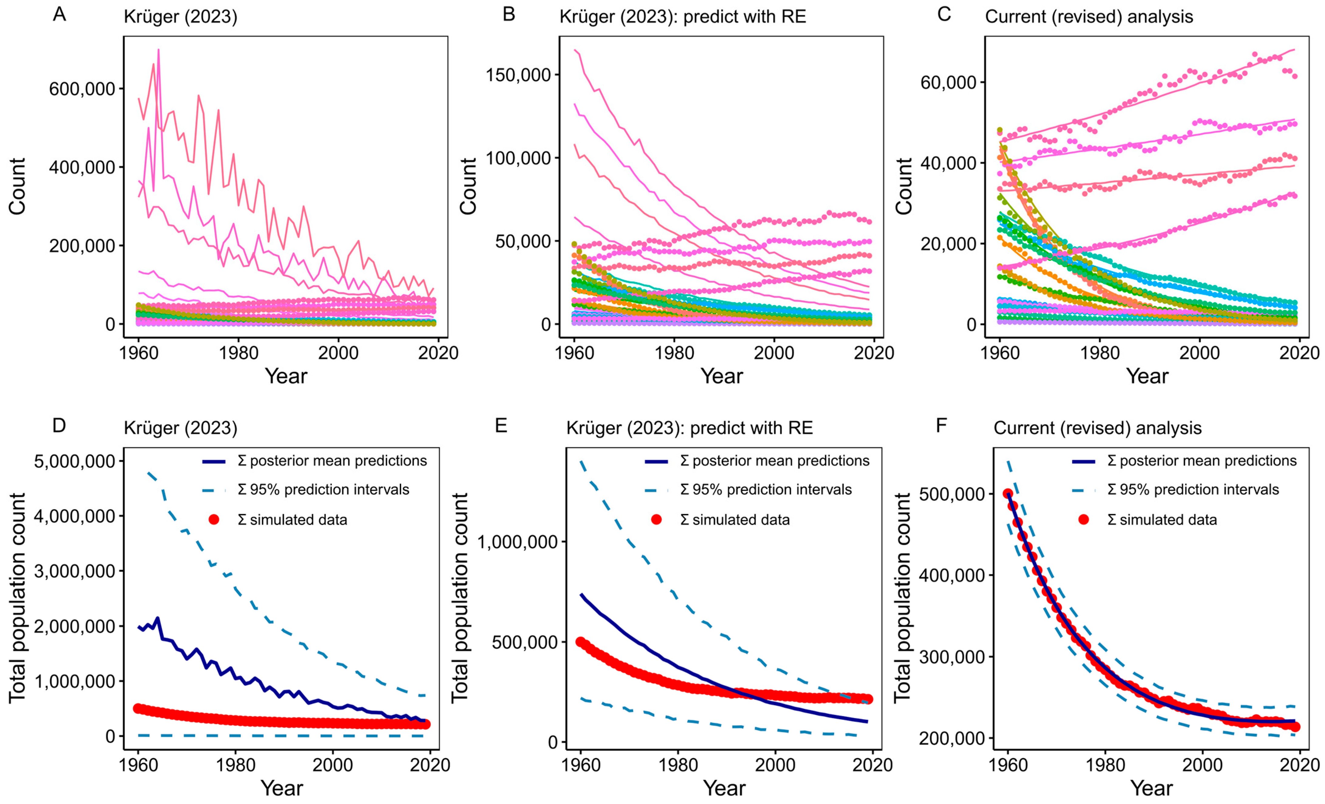
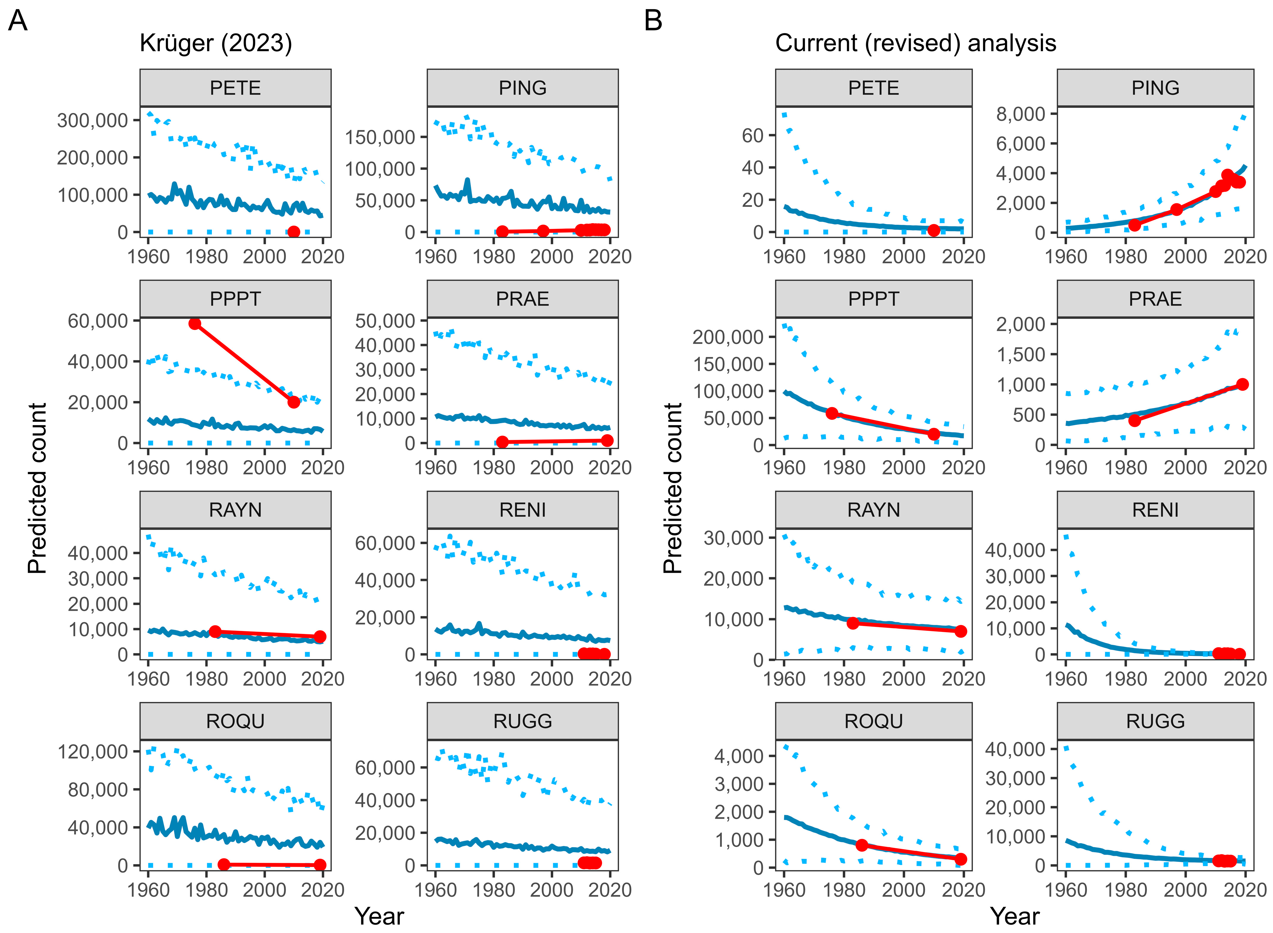
The second and more serious issue is lack of model fit. The Krüger [8] GLMM yielded extremely uncertain and biased estimates of the predicted abundance against observed values (Figure 2 and Figure 3). This simple model-checking procedure shows that the model’s predictions cannot support downstream inferences about long-term changes in chinstrap penguin abundance. The lack of model fit partly arose because the model did not allow the sites’ population trajectories to vary (see below) (Supplementary Code S2).

4. Modelling Penguin Population Trends with GLMMs: A Reanalysis

Krüger’s [8] GLMM analysis aimed to (i) quantify population-level trends of chinstrap penguins and (ii) examine the variation in those trends between sites, relating it to latitude. Unfortunately, the structure of that paper’s GLMM meant that, in principle, it was unable to address the latter question. Here, we illustrate why this is so, propose a model structure that can address the question, and briefly present the results from this model.
The data being modelled are nest counts from numerous sites in various years, with latitude available as a site-level covariate. More than one hundred sites with counts in at least two breeding seasons between 1965 and 2019 were considered. In MCMCglmm, Krüger [8] specified the model as:
MCMCglmm(nests ~ season_starting, random = ~us(1 + Lat):site_id,
rcov=~units, family = “poisson”, …)
where the first argument specifies the response and the fixed effects; season_starting is the temporal predictor (defined as the year in which a breeding season begins), and an intercept is implicit. The second argument describes the random effects; an intercept and latitude are included and their coefficients are allowed to vary by site. The function us() specifies the covariance structure between the random effects [13]. The third and fourth arguments specify a Poisson distribution for the response (with a log link) and independent and identically distributed (iid) count-level errors (on the log scale), accounting for possible overdispersion in the counts relative to the Poisson distribution.
To understand this model, we translate the MCMCglmm syntax into a mathematical model statement. First, we fix some notation. We let i index the counts, j index the sites, and j [ i ] denote the site at which the i th count was made. We use y i for the counts, t i for season_starting, and l j for Lat, the latitude of site j . Then, the Krüger [8] model is:
y i ~ P o i s s o n λ i l o g λ i = α + β t i + δ j [ i ] + θ j [ i ] l j [ i ] + ϵ i ,   f o r   i = 1 , ,   479 .
where the site-level random effects δ j and θ j associated with the intercept and latitude, respectively, are given a bivariate normal distribution with mean zero and full covariance matrix, and ϵ i is the count-level error.
The coefficient in the model that captures temporal trends is β . However, β is shared across sites, and therefore, it cannot be modelled in terms of the site-level covariate latitude. In fact, the inclusion of the site-level random effects δ j and θ j serve only to allow the intercept to vary by site (see Supplementary Text S5 and Supplementary Code S2 for an illustration using simulated data). The quantity δ j + θ j l j represents the site-level offset from the population-level intercept α . Moreover, the two parameters δ j , θ j are not separately identifiable, and this may partly explain the poor mixing of the MCMC chain.
The question of latitudinal variation in temporal trends can be addressed with a hierarchical model in which β is allowed to vary by site and is modelled in terms of latitude (see [17], Chapter 13, Section 13.1 for a very similar model and discussion). We consider one such model given by:
y i ~ P o i s s o n λ i l o g λ i = α j [ i ] + β j [ i ] t i + ϵ i ,   f o r   i = 1 , ,   479 α j = γ 0 α + γ 1 α l j + ϵ j α β j = γ 0 β + γ 1 β l j + ϵ j β
where the site-level errors ϵ α and ϵ β are again given a bivariate normal distribution with mean zero and a full covariance matrix. Thus, we have a random-intercept, random-slope model in which the intercept and slope vary by site and both are modelled in terms of the site-level covariate latitude. The coefficients γ 1 α and γ 1 β capture any relationships between latitude and counts and between latitude and temporal trends in counts, respectively.
To specify this model in MCMCglmm, substitute the equations for α j and β j into the expression for l o g ( λ i ) and rearrange as follows:
l o g λ i = γ 0 α + γ 1 α l j i + ϵ j i α + ( γ 0 β + γ 1 β l j i + ϵ j i β ) t i + ϵ i =   γ 0 α + γ 1 α l j i + γ 0 β t i + γ 1 β l j i t i   f i x e d   e f f e c t   t e r m s +   ϵ j i α + ϵ j i β t i r a n d o m   e f f e c t   t e r m s +   ϵ i     c o u n t   e r r o r
The γ   coefficients that do not depend on the site index j are specified as fixed effects, and the ϵ   coefficients that do are specified as random effects varying by site. The crucial term to capture latitudinal variation in temporal trends is the fourth term, which is specified as an interaction between latitude and time. The formula translates directly into the following MCMCglmm syntax:
MCMCglmm(nests ~ 1 + Lat + season_starting + Lat:season_starting,
random = ~us(1 + season_starting):site_id,
rcov=~units, family = “poisson”, …)

5. Predicting Penguin Population Trends with GLMMs

With mixed models, we must decide whether to include information about the random effects in the predictions (e.g., [18], Chapter 13, Section 13.5 and [19]). Here, and in [8], the aim was to predict nest counts in years with missing observations, for the same sites used to fit the GLMM. This problem is different from making predictions for new sites, and the nuances strongly affect the predicted counts (Figure 2). Krüger [8] marginalized the site effects in the prediction (the default option in predict.MCMCglmm) to obtain average nest counts across all sites (the predict.MCMCglmm syntax for our GLMM would be marginal = ~us(1 + season_starting):site_id). Population-average predictions are useful in some cases (e.g., to predict trends at sites that were not included in the analysis), but to capture site-level trends and to derive better estimates of overall population numbers, the random effects must be included when computing predictions (the argument inside the predict.MCMCglmm syntax is marginal = NULL) (Figure 2, Supplementary Code S3).
Krüger [8] did not propagate the substantial parameter uncertainty associated with the GLMM through to the overall trend prediction and to rates of population change, but this should be done. Therefore, predictions of population size must depend on the entire posterior distribution, and we should use the whole distribution (syntax posterior = “all”) rather than a single point (posterior = “mean”) when predicting with predict.MCMCglmm (e.g., [18], Chapter 4, Sections 4.3 and 4.4). The posterior mean discards the uncertainty in the posterior distribution, and this leads to overconfident predictions.
To assess whether predicted nest counts were reasonable, we plotted the posterior mean and 95% prediction interval (highlighting the region within which the model expected to find the most previous (or future) counts) against observed data for every site. We summed the site-level posterior prediction means and intervals to obtain the predicted overall population size for every year.
We did not attempt to replicate Krüger’s [8] approach of estimating population change, as that analysis did not propagate model and prediction uncertainty through to the estimates of population change. Instead, we used the entire posterior distribution ( y ~ ) (and not only its mean) to obtain estimates for percent change in population size over 30 years, as follows:
y ~ = 100   · y ~ t y ~ t 30 y ~ t 30 .
This gives a posterior distribution over y ~   from which we can obtain point estimates, credible intervals, or any other summary statistics related to the change in total population size. This method propagates model and prediction uncertainty to the estimates of population change and can be applied over any interval t .
Analyses of simulated and MAPPPD data showed that our GLMM specification was able to reasonably quantify variation in population trends between sites (Figure 2 and Figure 3) and relate it to latitude (Figure 4) (detailed results are given in Supplementary Codes S2 and S3 [simulated data] and Supplementary Codes S4–S6 [MAPPPD data]). Crucially, predictions from the fitted model agreed with the observed trends only when conditioned on the random effects (i.e., when predicting to the specific levels of the random effects).

6. How Sparse Is Too Sparse?

Extrapolations outside the range of observed data can easily lead to biased predictions [20]. Since there are almost no MAPPPD data from prior to 1970 (Figure 1), we do not recommend predicting chinstrap penguin population trends back to 1960 [8]. Although MAPPPD data have increased from the 1980s, the unbalanced nature of the counts at the site level amplifies the problem of extrapolation. For example, Krüger’s [8] analysis included several sites that were first counted after 2010—i.e., at these specific sites, predicted population sizes were extrapolated over more than 50 years.
Analysts of MAPPPD data that wish to reduce extrapolation beyond the range of observed data are confronted with a high number of “researcher degrees of freedom”—the different, reasonable (but subjective) data processing decisions that can be made. These decisions give rise to variations in the processed data used for modelling, and potentially the conclusions drawn (e.g., [21]). For example, in our revised analysis, we predicted population trends between 1980 and 2019 and evaluated the 30-year population change between 1990 and 2019 for three datasets with slightly different data inclusion criteria. Dataset 1 included all sites (n = 91) with at least two counts (with accuracy < 5) between 1980 and 2019 (Supplementary Code S4); dataset 2 contained sites (n = 71) with two or more counts (with accuracy < 5) over a period of at least 10 years between 1980 and 2019 (Supplementary Code S5); and dataset 3 comprised sites (n = 57) with at least one count (with accuracy < 5) prior to 2005 (i.e., within 15 years of 1990) and at least one count (with accuracy < 5) after 2004 (i.e., within 15 years of 2019) (Supplementary Code S6). Each of these case-study datasets were constructed according to subjective criteria that aimed to make use of as much data as possible while reducing extrapolations. Several other reasonable choices relating to data processing could have been made, potentially leading to different results.
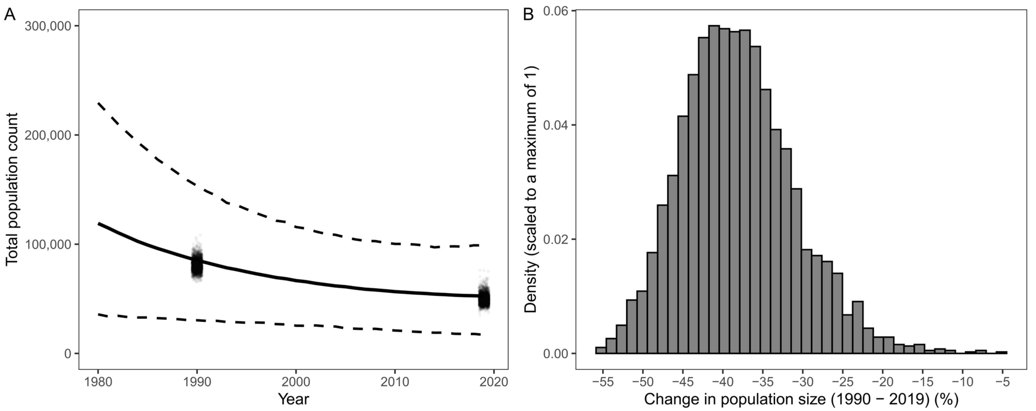
Our reanalysis (see Supplementary Codes S4–S6) mainly intends to show how uncertainty in model parameters can be propagated to population change estimates (see previous section), and how data selection criteria (as described above) can lead to substantial variation in estimates of population change. Our reanalysis found that there was a 59% (dataset 1), 43% (dataset 2), or 88% (dataset 3) probability that the aggregate abundance of the chinstrap penguin colonies included in each dataset decreased by at least 30% between 1990 and 2019. For dataset 3, the 90% posterior credible interval for the change in abundance from 1990 to 2019 indicated a decrease of between 26 and 49% (Figure 5), but no clear trend between colony decline and latitude was observed (Figure 4). It is important to note that these results (dataset 3) excluded the South Sandwich Islands (where populations are apparently stable [22]) as well as many of the largest colonies in the Antarctic Peninsula (e.g., Harmony Point on Nelson Island, Sandefjord Bay in the South Orkney Islands, Cape Wallace and Cape Garry on Low Island, and Baily Head on Deception Island). These large (and declining) colonies were excluded because their time series of nest count data was too sparse and/or uncertain to meet our data processing criteria.

7. Conclusions

Historical data on chinstrap penguin breeding population sizes are sparse and sometimes highly uncertain, making it hard to estimate true population trajectories. Krüger’s study [8] attempted to summarize the decline of chinstrap penguin populations—an important topic in the context of conservation management in the Southern Ocean—and the author’s ultimate conclusion about population vulnerability may even be perfectly correct. Unfortunately, a series of unintentional analytic errors undermine the validity of the findings. We show through reanalysis how improved statistical modelling can yield better predictions of chinstrap penguin population trends, at least within the range of observed data. Mixed model analyses are intricate, but good statistical protocols can help expose pitfalls and prevent incorrect model-based inference [23]. Ultimately, appropriate statistical support is required for evidence-based conclusions, and the assumptions and fit of every model must be checked (e.g., by comparing the model predictions against the observed data) before conclusions can be drawn [24].
Prediction uncertainty increases substantially as we move further from the observed data, even when models are correctly specified. Extrapolation and interpolation of chinstrap penguin population trends are difficult to avoid in the absence of systematic surveys, and it is important to incorporate prediction uncertainty when estimating population change. While historical population trends of chinstrap penguins will remain difficult to estimate, we are more optimistic about obtaining better inferences of contemporary trends. This optimism is due to recent increases in sampling (count data available in MAPPPD) and the potential for more accurate and precise penguin colony counts in the future (e.g., through remotely piloted aircraft [25]). Beyond monitoring trends, there is a real need to understand the drivers of population change in chinstrap penguins. Though labor-intensive, individual-based capture–recapture data [26] and integrated population model analysis [27] can identify the demographic parameters (e.g., reproduction, survival, dispersal) and external factors (e.g., environmental and fisheries-related variables) that drive population change. Collecting more data may be a crucial step toward a deeper understanding of the magnitude and underlying causes of population changes in chinstrap penguins. However, robust data analysis will be essential to draw meaningful conclusions that can enhance conservation and management effectiveness in the Antarctic Peninsula.

Supplementary Materials

The following supporting information can be downloaded at https://www.mdpi.com/article/10.3390/d16110651/s1, Supplementary Texts (S1 to S5) and Supplementary Code, provided as R Markdown (.Rmd) files and converted PDF documents: Supplementary Code S1—Krüger (2023) [8] data analysis and revised model fitting to this data set. Supplementary Code S2—Simulation study: Krüger (2023) [8] and revised model fitting and prediction. Supplementary Code S3—Simulation study with sparse data: Krüger (2023) [8] and revised model fitting and prediction. Supplementary Code S4—Dataset 1 (n = 91 sites): revised model fitting and prediction. Supplementary Code S5—Dataset 2 (n = 71 sites): revised model fitting and prediction. Supplementary Code S6—Dataset 3 (n = 57 sites): revised model fitting and prediction. References [28,29] are listed in the Supplementary Material.

Author Contributions

Conceptualization, W.C.O.; methodology, W.C.O., M.C. and M.N.; formal analysis, W.C.O.; validation, W.C.O., M.C. and M.N.; writing—original draft preparation, W.C.O.; writing—review and editing, W.C.O., M.C. and M.N. All authors have read and agreed to the published version of the manuscript.

Funding

This research received no external funding.

Data Availability Statement

Analysis code is available online as part of the Supplementary Materials. All data, code and fully reproducible workflows are also available as a live Github Repository (https://github.com/ChrisOosthuizen/ChinstrapTrends, accessed on 28 September 2024).

Conflicts of Interest

The authors declare no conflicts of interest.

References

  1. IUCN (International Union for Conservation of Nature). IUCN Red List Categories & Criteria, 2nd ed.; Version 3.1; IUCN: Gland, Switzerland, 2012. [Google Scholar]
  2. Paleczny, M.; Hammill, E.; Karpouzi, V.; Pauly, D. Population trend of the world’s monitored seabirds, 1950–2010. PLoS ONE 2015, 10, 0129342. [Google Scholar] [CrossRef] [PubMed]
  3. White, E.R. Minimum time required to detect population trends: The need for long-term monitoring programs. BioScience 2019, 69, 40–46. [Google Scholar] [CrossRef]
  4. Clark, J.S.; Bjørnstad, O.N. Population time series: Process variability, observation errors, missing values, lags, and hidden states. Ecology 2004, 85, 3140–3150. [Google Scholar] [CrossRef]
  5. Authier, M.; Galatius, A.; Gilles, A.; Spitz, J. Of power and despair in cetacean conservation: Estimation and detection of trend in abundance with noisy and short time-series. PeerJ 2020, 8, e9436. [Google Scholar] [CrossRef] [PubMed]
  6. Strycker, N.; Wethington, M.; Borowicz, A.; Forrest, S.; Witharana, C.; Hart, T.; Lynch, H.J. A global population assessment of the Chinstrap penguin (Pygoscelis antarctica). Sci. Rep. 2020, 10, 19474. [Google Scholar] [CrossRef] [PubMed]
  7. Humphries, G.R.W.; Naveen, R.; Schwaller, M.; Che-Castaldo, C.; McDowall, P.; Schrimpf, M.; Lynch, H.J. Mapping application for penguin populations and projected dynamics (MAPPPD): Data and tools for dynamic management and decision support. Polar Rec. 2017, 53, 160–166. [Google Scholar] [CrossRef]
  8. Krüger, L. Decreasing Trends of Chinstrap Penguin Breeding Colonies in a Region of Major and Ongoing Rapid Environmental Changes Suggest Population Level Vulnerability. Diversity 2023, 15, 327. [Google Scholar] [CrossRef]
  9. Warwick-Evans, V.; Kelly, N.; Dalla Rosa, L.; Friedlaender, A.; Hinke, J.T.; Kim, J.H.; Trathan, P.N. Using seabird and whale distribution models to estimate spatial consumption of krill to inform fishery management. Ecosphere 2022, 13, e4083. [Google Scholar] [CrossRef]
  10. R Core Team. R: A Language and Environment for Statistical Computing; R Foundation for Statistical Computing: Vienna, Austria, 2022; Available online: https://www.R-project.org/ (accessed on 5 October 2023).
  11. Hill, S.L.; Atkinson, A.; Pakhomov, E.A.; Siegel, V. Evidence for a decline in the population density of Antarctic krill Euphausia superba still stands. A comment on Cox et al. J. Crustac. Biol. 2019, 39, 316–322. [Google Scholar] [CrossRef]
  12. Lynch, H.J.; Naveen, R.; Trathan, P.N.; Fagan, W.F. Spatially integrated assessment reveals widespread changes in penguin populations on the Antarctic Peninsula. Ecology 2012, 93, 1367–1377. [Google Scholar] [CrossRef]
  13. Hadfield, J.D. MCMC methods for multi-response generalized linear mixed models: The MCMCglmm R package. J. Stat. Softw. 2010, 33, 1–22. [Google Scholar] [CrossRef]
  14. Zuur, A.F.; Ieno, E.N.; Walker, N.J.; Saveliev, A.A.; Smith, G.M. Mixed Effects Models and Extensions in Ecology with R; Springer: New York, NY, USA, 2009. [Google Scholar]
  15. Gelman, A.; Carlin, J.B.; Stern, H.S.; Dunson, D.B.; Vehtari, A.; Rubin, D.B. Bayesian Data Analysis; CRC Press: Boca Raton, FL, USA, 2013. [Google Scholar]
  16. Conn, P.B.; Johnson, D.S.; Williams, P.J.; Melin, S.R.; Hooten, M.B. A guide to Bayesian model checking for ecologists. Ecol. Monogr. 2018, 88, 526–542. [Google Scholar] [CrossRef]
  17. Gelman, A.; Hill, J. Data Analysis Using Regression and Multilevel/Hierarchical Models; Cambridge University Press: Cambridge, UK, 2006. [Google Scholar]
  18. McElreath, R. Statistical Rethinking: A Bayesian Course with Examples in R and Stan, 2nd ed.; Chapman and Hall/CRC: Boca Raton, FL, USA, 2020. [Google Scholar]
  19. Heiss, A. A Guide to Correctly Calculating Posterior Predictions and Average Marginal Effects with Multilievel Bayesian Models. 10 November 2021. Available online: https://www.andrewheiss.com/blog/2021/11/10/ame-bayes-re-guide/ (accessed on 1 October 2023).
  20. Conn, P.B.; Johnson, D.S.; Boveng, P.L. On extrapolating past the range of observed data when making statistical predictions in ecology. PLoS ONE 2015, 10, e0141416. [Google Scholar] [CrossRef] [PubMed]
  21. Gould, E.; Fraser, H.S.; Parker, T.H.; Nakagawa, S.; Griffith, S.C.; Vesk, P.A.; Fidler, F.; Hamilton, D.G.; Abbey-Lee, R.N.; Abbott, J.K.; et al. Same data, different analysts: Variation in effect sizes due to analytical decisions in ecology and evolutionary biology. EcoEvoRxiv online. 2023. [Google Scholar] [CrossRef]
  22. Lynch, H.J.; White, R.; Naveen, R.; Black, A.; Meixler, M.S.; Fagan, W.F. In stark contrast to widespread declines along the Scotia Arc, a survey of the South Sandwich Islands finds a robust seabird community. Polar Biol. 2016, 39, 1615–1625. [Google Scholar] [CrossRef]
  23. Silk, M.J.; Harrison, X.A.; Hodgson, D.J. Perils and pitfalls of mixed-effects regression models in biology. PeerJ 2020, 8, e9522. [Google Scholar] [CrossRef]
  24. Popovic, G.; Mason, T.J.; Drobniak, S.M.; Marques, T.A.; Potts, J.; Joo, R.; Altwegg, R.; Burns, C.C.I.; McCarthy, M.A.; Johnston, A.; et al. Four principles for improved statistical ecology. Methods Ecol. Evol. 2024, 15, 266–281. [Google Scholar] [CrossRef]
  25. Hodgson, J.C.; Mott, R.; Baylis, S.M.; Pham, T.T.; Wotherspoon, S.; Kilpatrick, A.D.; Segaran, R.R.; Reid, I.; Terauds, A.; Koh, L.P. Drones count wildlife more accurately and precisely than humans. Methods Ecol. Evol. 2018, 9, 1160–1167. [Google Scholar] [CrossRef]
  26. Hinke, J.T.; Salwicka, K.; Trivelpiece, S.G.; Watters, G.M.; Trivelpiece, W.Z. Divergent responses of Pygoscelis penguins reveal a common environmental driver. Oecologia 2007, 153, 845–855. [Google Scholar] [CrossRef] [PubMed]
  27. Weegman, M.D.; Arnold, T.W.; Dawson, R.D.; Winkler, D.W.; Clark, R.G. Integrated population models reveal local weather conditions are the key drivers of population dynamics in an aerial insectivore. Oecologia 2017, 185, 119–130. [Google Scholar] [CrossRef] [PubMed]
  28. Schweinsberg, M.; Feldman, M.; Staub, N.; van den Akker, O.R.; van Aert, R.C.; Van Assen, M.A.; Liu, Y.; Althoff, T.; Heer, J.; Kale, A.; et al. Same data, different conclusions: Radical dispersion in empirical results when independent analysts operationalize and test the same hypothesis. Organ. Behav. Hum. Decis. Process. 2021, 165, 228–249. [Google Scholar] [CrossRef]
  29. Croxall, J.P.; Kirkwood, E.D. The Distribution of Penguins on the Antarctic Peninsula and Islands of the Scotia Sea; British Antarctic Survey: Cambridge, UK, 1979. [Google Scholar]
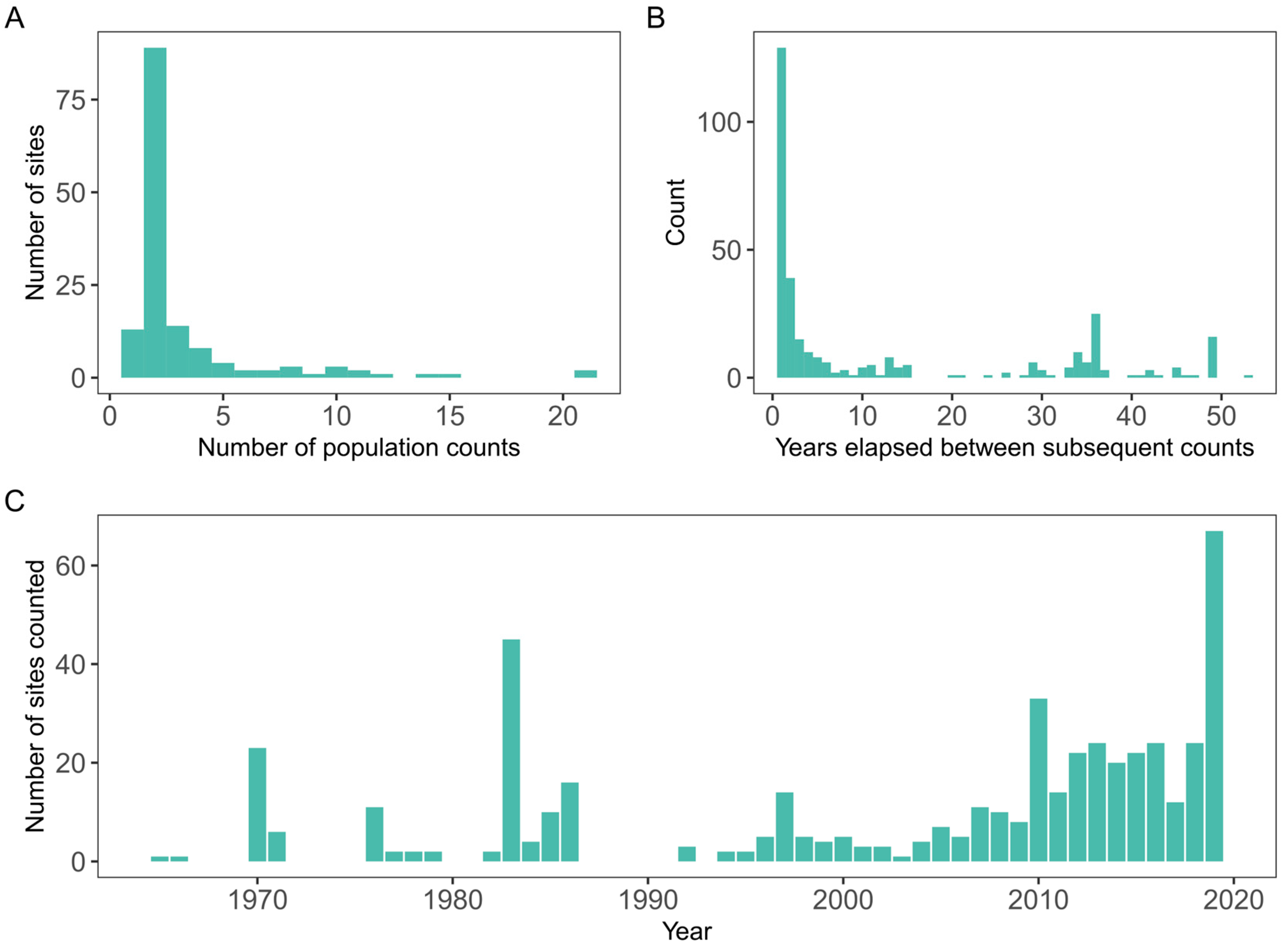
Figure 1. Distribution of chinstrap penguin nest count data (1965–2019) analyzed in Krüger (2023). (A) In total, 133 sites had multiple counts, but most sites were only counted twice. Sites with a single count were excluded from GLMM analysis (but 13 sites with a single non-zero count unintentionally remained in the data). (B) While year-on-year counts at a site were common, decades lapsed between successive counts at some sites. (C) Count frequencies were highest after 2010, with high effort also occurring in 1970 and 1983.
Diversity 16 00651 g001
Figure 2. Analysis of simulated data (annual counts [1960–2019] at 26 sites) showing that Krüger (2023)’s [8] GLMM poorly predicts population trends. (A) Site-level predictions (lines, colored by site) obtained by fitting Krüger (2023)’s GLMM to simulated data (points) and predicting without taking random effects into account (corresponding to the analysis in that paper). (B) Site-level predictions (lines) obtained by fitting Krüger (2023)’s GLMM to simulated data (points) and predicting with random effects. (C) Site-level predictions (lines) obtained by fitting our revised GLMM to the same simulated data (points) and predicting while taking random effects into account. (DF) Total population abundance (aggregate of simulated data across all sites) (in red) and predicted total population (sum of site-level mean prediction and 95% prediction intervals) (in blue) obtained using the Krüger (2023) GLMM specification (D,E) and from our revised analysis (F).
Diversity 16 00651 g002
Figure 3. Observed and predicted chinstrap penguin nest counts at a subset of sites in the Antarctic Peninsula. The results presented in this figure were obtained using Krüger (2023)’s [8] input data, and predictions were made back to 1960 to correspond with that paper (results for all sites included in Krüger (2023) are given in Supplementary Code S1). Blue solid lines are the predicted abundance (posterior mean) obtained following Krüger (2023) (A) and our revised model specification (B). Light blue dots are the 95% prediction intervals obtained through posterior predictive simulation. Red points are the observed counts (connected with a red line).
Diversity 16 00651 g003
Figure 4. Random effects slope, indicating population change relative to latitude for 57 chinstrap penguin populations (dataset 3, revised GLMM) in the Antarctic Peninsula. Points above the dotted line indicate colony increases; points below the dotted line represent colony decreases. A simple generalized additive model fitted to the points (solid blue line and 95% confidence interval in grey shading) indicated no trend in population change with latitude for these specific colonies.
Diversity 16 00651 g004
Figure 5. Predicted population change for 57 chinstrap penguin populations in the Antarctic Peninsula. These populations had at least one count prior to 2005 (i.e., within 15 years of 1990) and at least one count after 2004 (i.e., within 15 years of 2019). (A) Population trend between 1980 and 2019. The solid line is the predicted average abundance (posterior mean) and dotted lines are the 95% prediction interval. The point clouds represent the distribution of average population size in 1990 and 2019 (the entire posterior distribution for the mean). (B) For this sample of sites, the 90% posterior probability was a decrease of between 26% and 49% from 1990 to 2019.
Diversity 16 00651 g005
Table 1. Summary of main analytic differences between Krüger (2023) [8] and the current study. Some differences are related to ‘researcher degrees of freedom’—i.e., different analyses choices, where multiple reasonable options may exist. These are given in italics.
Analysis StepKrüger (2023)Current Study
MAPPPD dataIgnored count uncertainty.Excluded counts with very high uncertainty (“to an order of magnitude”; MAPPPD level 5) to mitigate the impact of potentially extreme observation errors on population trends. While we do not address this issue here, count uncertainty should ideally also be accounted for in the remaining data.
MAPPPD dataRemoved nest counts with unknown ‘day’ and ‘month’ of count (day/month not used otherwise).Kept nest counts where ‘day’ and ‘month’ of count were unknown to increase the initial sample size.
MAPPPD dataRemoved ‘true zeros’ (counts with zero nests).Kept ‘true zeros’ (counts with zero nests).
MAPPPD dataConsidered all data between 1965 and 2019.Limited data to the period with most observations (1980–2019).
MAPPPD dataConsidered all sites with two or more counts (but 13 sites with a single non-zero count unintentionally remained in the GLMM dataset).Sites with two or more counts were considered, but case studies attempted to avoid extreme extrapolation of population predictions at sites where counts covered only a small fraction of the time series.
Model fittingIncorrect GLMM structure for fixed and random effects.Improved GLMM structure for fixed and random effects.
Model fittingDid not standardize covariates, encumbering model fitting and convergence.Standardized covariates to mean 0, standard deviation 1 before model fitting.
Model fittingUsed default MCMCglmm sampling parameters.Increased the MCMC sampling and burn-in period (though this was not strictly required).
Model evaluationDid not evaluate MCMC diagnostics and model fit.Evaluated the model’s effective sample size and mixing (trace plots) and plotted model predictions against observed values.
Model
inference
Random intercepts were incorrectly presented as random slopes (population change), with standard deviations halved.Random slopes give latitudinal variation in population change.
Model
prediction
Prediction did not include random effects.Predicted with random effects to obtain accurate site-level predictions.
Model
prediction
Prediction did not propagate model uncertainty (assumed the posterior mean was the true size of the population). Used the entire posterior sample to propagate uncertainty of prediction to rates of population change.
Model
prediction
Extrapolated population predictions far beyond observed data (back to 1960).Attempted to limit extrapolation of population trends beyond observed data. Limited predictions to 1980–2019 and calculated 30-year population change between 1990 and 2019.
Disclaimer/Publisher’s Note: The statements, opinions and data contained in all publications are solely those of the individual author(s) and contributor(s) and not of MDPI and/or the editor(s). MDPI and/or the editor(s) disclaim responsibility for any injury to people or property resulting from any ideas, methods, instructions or products referred to in the content.